Chaotic dynamics of three-dimensional Hénon maps that originate from a homoclinic bifurcation

Abstract

We study bifurcations of a three-dimensional diffeomorphism, $g_{0}$, that has a quadratic homoclinic tangency to a saddle-focus fixed point with multipliers $(\lambda e^{i\varphi},\lambda e^{-i\varphi},\gamma)$, where $0<\lambda<1<|\gamma|$ and $|\lambda^{2}\gamma|=1$. We show that in a three-parameter family, $g_{\varepsilon}$, of diffeomorphisms close to $g_{0}$, there exist infinitely many open regions near $\varepsilon=0$ where the corresponding normal form of the first return map to a neighborhood of a homoclinic point is a three-dimensional Hénon-like map. This map possesses, in some parameter regions, a “wild-hyperbolic” Lorenz-type strange attractor. Thus, we show that this homoclinic bifurcation leads to a strange attractor. We also discuss the place that these three-dimensional Hénon maps occupy in the class of quadratic volume-preserving diffeomorphisms.

1 Introduction

In this paper we are concerned with the study of the three-dimensional map $(\bar{x},\bar{y},\bar{z})=f(x,y,z)\in{\mathbb{R}}^{3}$ defined by

$$\begin{array}[]{l}\bar{x}=y,\;\;\bar{y}=z,\;\;\bar{z}=M_{1}+Bx+M_{2}y-z^{2}\;,\end{array}$$ (1)

with three parameters, $M_{1}$, $M_{2}$, and $B$. This map is a natural generalization of the famous two-dimensional Hénon map [H7́6]; indeed, like the latter, the map (1) is quadratic, has constant Jacobian $\det(Df)\equiv B$ and moreover, when $B=0$, reduces to the two-dimensional Hénon map. Therefore, it is natural to call (1) the “3D Hénon map.” We will study a number of properties of (1), including:

1. its nontrivial dynamics and, most importantly, the existence of wild-hyperbolic strange attractors;

2. its origination in homoclinic bifurcations;

3. its structure as a member of the family of three-dimensional quadratic maps with constant Jacobian.

Three-dimensional maps have not been as widely studied as one- and two-dimensional maps, though in recent years there has been a considerable increase in their study. One of important reasons for this fact is that multi-dimensional dynamical systems (the dimension of the phase space is at least four for flows and three for maps) can exhibit complicated dynamics that is decidedly distinct from lower-dimensional cases. In particular they can possess a new variety of strange attractor called a wild-hyperbolic attractor [ST98].

Wild-hyperbolic attractors have no uniform hyperbolic structure; moreover, they may contain homoclinic tangencies and coexisting periodic orbits of different types. However, these attractors contain no stable invariant subsets such as attracting periodic orbits. Most crucially, the latter property holds for open regions in the space of smooth dynamical systems. Thus, wild-hyperbolic attractors are very interesting objects and their detection in concrete models is a fundamental problem of nonlinear dynamics.

Most of the strange attractors occurring in two-dimensional, smooth maps (or three-dimensional flows) are not structurally stable since they possess homoclinic tangencies. For such systems, even though the orbits are observed to be quite chaotic for some parameter values, very small changes in the parameters may destroy the aperiodicity and give rise to periodic behavior. Such parameter regions are called stability windows. Even if these windows are not “observable” in numerical computations, their appearance (under arbitrarily small perturbations) is inevitable because of the prevalence of homoclinic tangencies. Such attractors were called quasi-attractors in [AS83]. One of the most challenging problems in dynamical systems is to distinguish aperiodic motion from extremely long periodic motion. Moreover, since most of the chaotic attractors we see in applications are definitely quasi-attractors, it is unclear in which sense they are chaotic, or how one can define and measure the ”probability” for a quasi-attractor to be chaotic.

However, it is well-known that there are strange attractors that are free of these problems; for example, hyperbolic attractors and the Lorenz attractor. Though the latter is not structurally stable [GW79],[ABS82] (in contrast to hyperbolic attractors) it contains no stable periodic orbits, every orbit in it has positive maximal Lyapunov exponent, etc. Moreover, these properties are robust [ABS77],[GW79]. The reason is that Lorenz attractor possesses a pseudo-hyperbolic structure. In terms of Turaev and Shilnikov [ST98] this means that the following properties hold:

1. there is a direction in which the flow is strongly contracting (”strongly” means that any possible contraction in transverse directions is always strictly weaker); and

2. transverse to this direction the flow expands areas.

The robustness of pseudo-hyperbolicity ensures the robustness of the chaotic behavior of orbits in the Lorenz attractor. Moreover, pseudo-hyperbolicity is maintained even for (small, indeed) time-periodic perturbations so that a periodically forced Lorenz attractor is an example of a genuinely “strange” attractor since it contains no stable invariant subsets (for more discussion see [SST93],[GOST05],[TS05]). However it is necessary to note that homoclinic tangencies arise inevitably under such perturbations. Consequently systems with periodically forced Lorenz attractors fall into Newhouse regions and demonstrate an extremely rich dynamics [GTS93],[GTS99]. Such attractors were called wild-hyperbolic attractors in [ST98]; in this paper the theory of wild-pseudo-hyperbolic attractor was discussed and an example of a wild-hyperbolic spiral attractor was constructed.

Generalizing these ideas, we say that wild-hyperbolic attractors possess the following two main properties that distinguish them from other attractors: (1) wild-hyperbolic attractors allow homoclinic tangencies (hence, they belong to Newhouse regions); (2) every such attractor and all nearby attractors (in the $C^{r}$-topology with $r\geq 2$) have no stable periodic orbits.

One of the most felicitous properties of wild-hyperbolic attractors is that they can be created in local bifurcations of periodic orbits; in particular, when the orbit has three or more Floquet multipliers on the unit circle [SST93]. Consequently, the construction of wild-hyperbolic attractors in concrete models is possible when the model contains sufficiently many parameters to permit such a degeneracy. Indeed, the map (1) is sufficiently complex and has been shown to possess wild-hyperbolic attractors [GOST05]. Moreover, numerical simulations have shown that these attractors persist in quite big parameter domains and can be order-one in size [GOST05].

In §6 we will show that (1) has a small, wild-hyperbolic Lorenz attractor in a (small) parameter domain near the point $(M_{1},M_{2},B)=(-1/4,1,1)$ at which a fixed point with multipliers $(-1,-1,+1)$ exists. The general case of fixed points with such a triplet of multipliers was considered in [SST93], where it was shown that two distinct cases occur. One of these cases has a local flow normal form that coincides with the Shimitsu-Marioka system (see (33)). This system has a Lorenz attractor in some parameter domains [Shi86],[Shi93]. As was noted in [ST98] a periodically forced Lorenz system (when the perturbation is rather small) can give rise to a wild-hyperbolic attractor. Moreover, this does not destroy the pseudo-hyperbolicity of the attractor [ST98],[GOST05]. Note that the flow normal form only approximates the map and, since the residual terms are exponentially small in time, it is reasonable that the map will have a wild-hyperbolic attractor (which is small, in fact, because the approximation must be very good), see more discussions in [GOST05].

The second property of (1) that we mentioned above is that this map can arise as a local normal form for multi-dimensional systems with a homoclinic tangency. This shows that such maps are not exotic and gives a reason for an extensive study of their properties.

It is well-known that quadratic maps appear naturally when studying bifurcations of quadratic homoclinic tangencies [GS72],[GS73],[TLY86],[GTS93],[GST03]. They appear as normal forms of rescaled first return maps to the neighborhood of a point on the homoclinic orbit. There are four standard forms for such one- and two-dimensional “homoclinic maps:”

1. $\bar{y}=M_{1}-y^{2}$ (the logistic map);

2. $(\bar{x},\bar{y})=(y,M_{1}-Bx-y^{2})$ (the standard Hénon map);

3. $(\bar{x},\bar{y})=(y,M_{1}+M_{2}y-x^{2})$ (the Mira map);

4. $(\bar{x},\bar{y})=(y,M_{1}-Bx-y^{2}+\varepsilon_{k}^{1}xy+\varepsilon_{k}^{2}y^{3})$ (a generalized Hénon map).

The third case is a two-dimensional endomorphism and is one of the well-studied polynomial maps (see, e.g. [MGBC96]); we call it the “Mira map” following [GST03]). The fourth case can be obtained as a small perturbation (due to $\varepsilon_{k}^{1,2}$-terms) of the standard Hénon map. This map was obtained in a study of bifurcations of two-dimensional diffeomorphisms with a homoclinic tangency to a saddle fixed point (with unit Jacobian) [GG00],[GG04].

The 3D Hénon map (1) is absent from this list, and in §3–§4 we will fill this gap.

In §3 we study bifurcations of a three-dimensional diffeomorphism with quadratic homoclinic tangency to a saddle-focus fixed point. For a three-dimensional map, such points can be of two types: $(2,1)$ or $(1,2)$ (sometimes called type A and type B, respectively). Recall that $(k,l)$ saddle is a fixed point with $\dim(W^{s})=k$, $\dim(W^{u})=l$, and $k+l=n$. In our case the two-dimensional manifold will be assumed to correspond to a complex conjugate pair of multipliers. We will consider the case where the the product the absolute value of the multipliers, $P_{0}$ is one.

The bifurcations in the general case, where $P_{0}\neq 1$, were studied in [GST96],[GST03]. We will use their “rescaling method” to study our case as well. The essence of this method is that a suitable change of coordinates and parameters in a neighborhood of the homoclinic orbit is found to bring the map into a standard form. If the homoclinic tangency is assumed to be quadratic the resulting map is also typically quadratic. For example, for a type $(2,1)$ saddle-focus with $P_{0}<1$, the rescaled first return maps coincide with the standard Hénon map up to asymptotically small terms (when the time of return tend to infinity). For a saddle-focus of type $(1,2)$, the corresponding rescaled first return map is the Mira map. Note the condition $P_{0}<1$ leads to maps that are effectively two-dimensional; consequently all three-dimensional volumes near the fixed point are collapsed. This is not the case when $P_{0}=1$ for the unperturbed map when three-dimensional rescaled maps can appear a priori. Indeed, we will show that when $P_{0}=1$ the map (1) occurs as the normal form of the rescaled map for type $(2,1)$ saddle-focus; and for the type $(1,2)$ case the corresponding normal form is

$$\begin{split}\bar{x}=y,\;\;\bar{y}=z,\;\;\bar{z}=M_{1}+Bx+M_{2}z-y^{2},\end{split}$$ (2)

Both (1) and (2) are quadratic three-dimensional maps with constant Jacobian $J\equiv B$. It is natural to call them the three-dimensional Hénon maps of the first and second kind, respectively.

The quadratic 3D Hénon maps are elements of the group of polynomial automorphisms. The study of the dynamics of polynomial mappings has a long history applied dynamics; for example, they often used in the study of particle accelerators [DA96]. The study of Cremona maps, i.e., polynomial maps with constant Jacobian, also has intrinsic mathematical interest [Eng58]. An interesting mathematical problem is to obtain a normal form for an arbitrary degree-$d$ Cremona map. This problem is unsolved; the major obstruction is that it is not known in general that such a map has a polynomial inverse. This is the content of the much studied, “Jacobian conjecture”:

Conjecture (O.T. Keller (1939)).

Let $f:{\mathbb{R}}^{n}\rightarrow{\mathbb{R}}^{n}$ be a Cremona map. Then $f$ is bijective and has a polynomial inverse.

This conjecture is still open.

The set of polynomial maps with polynomial inverses is called the affine Cremona group. For the case of the plane, the structure of this group was obtained by Jung [Jun42]. Jung’s theorem states that planar polynomial diffeomorphisms are “tame;” that is, they can be written as a finite composition of “elementary” (or triangular) and affine maps. More recently Friedland and Milnor [FM89] showed that any map in this group is either conjugate to a composition of generalized Hénon maps,

$$\bar{x}=y\;,\;\bar{y}=-Bx+p(y)\;,$$

where $p(y)$ is a polynomial and $B\neq 0$, or else the map is dynamically trivial.

Not much is known about the structure of the affine Cremona group for higher dimensions, though it was recently proved that the three-dimensional Cremona map

$$\begin{split}\bar{x}&=x-2y(xz+y^{2})-z(xz+y^{2})^{2}\;,\\ \bar{y}&=y+z(xz+y^{2})\;,\\ \bar{z}&=z\;,\end{split}$$

is not tame [SU04]. Thus the normal form for the 3D affine Cremona group must consist of more than tame maps. However, it is still possible that the nontame maps are dynamically trivial, like the above example.

Another interesting problem concerns the approximation of smooth diffeomorphisms by polynomial diffeomorphisms. One result along this direction is for the class of $C^{\infty}$ symplectic diffeomorphisms, which, as Turaev has shown [Tur03], can be approximated by compositions of the symplectic Cremona maps

$$\bar{x}=x_{0}+y\;,\;\bar{y}=-x+\nabla p(y)\;,$$

where $x,y,x_{0}\in{\mathbb{R}}^{n}$ and $p$ is a polynomial. Related approximation methods are used in the study of particle accelerators [DA96], and results have also been obtained for analytic symplectic maps [For96].

Some work has been done on finding normal forms for quadratic symplectic and quadratic volume-preserving maps. Moser showed that every quadratic symplectic map in ${\mathbb{R}}^{2n}$ can be written as the composition of an affine symplectic map and a symplectic shear [Mos94]. For the four-dimensional case, he obtained a normal form. For the case of volume-preserving maps, it was shown in [LM98],[LLM99] that any quadratic three-dimensional, volume-preserving map whose inverse is also quadratic and whose dynamics is non-trivial can be transformed (by affine transformations) to the form

$$\begin{split}\bar{x}&=y,\;\;\bar{y}=z,\;\;\\ \bar{z}&=M_{1}+Bx+M_{2}^{1}y+M_{2}^{2}z+ay^{2}+byz+cz^{2},\end{split}$$ (3)

where $B=1$, $|a+b+c|=1$ and one of the parameters $M_{2}^{1}$ or $M_{2}^{2}$ can be eliminated (by a coordinate shift). By analogy with the planar results, there are two additional cases but they have trivial dynamics (see §7). We also note that it is not hard to construct three-dimensional quadratic diffeomorphisms that do not fall into this classification because they have an inverse of higher degree. For example, the diffeomorphism

$$\bar{x}=x\;,\;\bar{y}=y+x^{2}\;,\;\bar{z}=z+y^{2}\;,$$

has a quartic inverse.

Note that both of the maps (1) and (2) fall into the form (3). Thus the results of [LM98] show that when $B=1$ both of the 3D Hénon maps occur as normal forms for quadratic elements of the affine Cremona group. Moreover, even when $B\neq 1$ the map (2) is a normal form for a certain class of quadratic maps [Tat01]. Tatjer showed that every quadratic map, $f$, for which $f\circ f$ is also quadratic, but has no invariant linear foliation is linearly conjugate to (2). In §2, we will generalize the results of [LM98] to show that (3) is the the normal form for quadratic diffeomorphisms with quadratic inverses when $B\neq 1$ as well.

2 Statement of Results

Consider a three-dimensional diffeomorphism $g_{0}\in C^{r}({\mathbb{R}}^{3})$ for some $r\geq 5$ that satisfies the following conditions (see Fig. 1):

1. $g_{0}$ has a type $(2,1)$ saddle-focus fixed point $O$ with multipliers $(\lambda_{0}e^{i\varphi_{0}},\lambda_{0}e^{-i\varphi_{0}},\gamma_{0})$ where $0<\lambda_{0}<1<|\gamma_{0}|$ (w.l.o.g. $0<\varphi_{0}<\pi$),;

2. $P_{0}\equiv|J_{0}|=|\lambda_{0}^{2}\gamma_{0}|=1$.

3. The stable, $W^{s}$, and unstable, $W^{u}$, invariant manifolds of the fixed point $O$ have a quadratic homoclinic tangency at the points of a homoclinic orbit $\Gamma_{0}$.

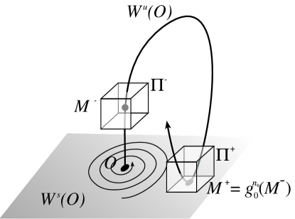
Figure 1: Geometry of the homoclinic orbit to a type $(2,1)$ saddle-focus for the map $g_{0}$ under assumputions (A)-(C).

Diffeomorphisms that are close to $g_{0}$ and satisfy conditions (B) and (C) comprise, in the space of $C^{r}$ diffeomorphisms, a codimension-two, locally-connected surface ${\cal H}$—the bifurcation surface.

Our main problem is to study bifurcations of periodic orbits in families of diffeomorphisms that transversely cross ${\cal H}$. We denote such a family by $g_{\varepsilon}$ so that $g_{0}$ satisfies (A)-(C). The first question that arises is the optimal choice of the governing parameters $\varepsilon$. It is evident that the set of such parameters must include both a parameter $\mu=\varepsilon_{1}$ of the splitting of the initial quadratic homoclinic tangency and a parameter $\varepsilon_{2}$, similar to $\varepsilon_{2}=P_{\varepsilon}-1$, that varies the Jacobian of the saddle-focus fixed point. However, it was shown in [Gon00] that diffeomorphisms on ${\cal H}$ possess continuous (topological) conjugacy invariants on the set of non-wandering orbits, so-called $\Omega$-moduli. The most important modulus is the angular argument $\varphi$ of the complex multipliers of the saddle-focus (see §4). By definition, $\Omega$-moduli are natural governing parameters. Therefore, we include the $\Omega$-modulus $\varphi$ into the set of governing parameters. Thus, we take as the third parameter $\varepsilon_{3}=\varphi-\varphi_{0}$.

More generally, we must consider a three-parameter family $g_{\varepsilon}$, $\varepsilon=(\varepsilon_{1},\varepsilon_{2},\varepsilon_{3})$, that is transversal to ${\cal H}$ at $\varepsilon=0$ and such that

$$\det\left(\frac{\partial(\varepsilon_{1},\varepsilon_{2},\varepsilon_{3})}{\partial(\mu,J,\varphi)}\right)\neq 0.$$

Consider a sufficiently small and fixed neighbourhood $U$ of the orbit $\Gamma_{0}$. It can be represented as a union of a small neighbourhood $U_{0}$ of $O$ with a number of small neighbourhoods of those points of $\Gamma_{0}$ which do not belong to $U_{0}$. In the family $g_{\varepsilon}$ we study bifurcations of single-round periodic orbits from $U$—that is orbits periodic that enter $U_{0}$ exactly once. Every point of such an orbit of period $k$ can be considered as a fixed point of the corresponding first return map $g^{k}_{\varepsilon}$ along orbits lying in $U$. In §4, we will prove the following result about the form of this first return map in some domains of the parameters.

Theorem 1.

Let $g_{\varepsilon}$ be the three parameter family defined above. Then, in any neighborhood of the origin, $\varepsilon=0$, of the space of parameters, there exist infinitely many open domains, $\Delta_{k}$, such that the first return map $g^{k}_{\varepsilon}$ takes the form

$$\begin{array}[]{l}\bar{X}=Y+o(1)_{k\to+\infty}\;,\\ \bar{Y}=Z+o(1)_{k\to+\infty}\;,\\ \bar{Z}=M_{1}+BX+M_{2}Y-Z^{2}+o(1)_{k\to+\infty}\;,\\ \end{array}$$ (4)

where $(X,Y,Z)$ are rescaled coordinates and the domains of definition of the new coordinates and the parameters $(M_{1},M_{2},B)$ are arbitrarily large and cover, as $k\to\infty$, all finite values. Furthermore, the Jacobian, $B$, is positive or negative depending on the orientability of the map $g^{k}_{\varepsilon}$. The terms denoted $o(1)$ are functions (of the coordinates and parameters) that tend to zero as $k\to+\infty$ along with all derivatives up to order $r-2$.

Theorem 1 shows that the 3D Hénon map (1) is a normal form for this homoclinic bifurcation, since it appears when we omit the $o(1)$-terms in (4). We will see that the new parameters $M_{1},M_{2}$ and $B$ can be given as functions of $\varepsilon=(\mu,\varphi-\varphi_{0},P_{\varepsilon}-1)$ by

$$M_{1}\sim\gamma^{3k}(\mu+{\cal O}(\lambda^{k}))\;,\;M_{2}\sim(\lambda\gamma)^{k}\cos(k\varphi+\beta)\;,\;B\sim(\lambda^{2}\gamma)^{k}$$

where $\beta$ is some coefficient (an invariant of $g_{0}$) and $(\lambda(0),\gamma(0))\equiv(\lambda_{0},\gamma_{0})$. The exact relations will be given in formulas (20), (25) and (27) below. Thus, we can study the bifurcations of single round periodic orbits in the family $g_{\varepsilon}$, when $\varepsilon\in\Delta_{k}$, by studying the bifurcations of fixed points of the 3D Hénon map (1).

Certainly, the problem of studying bifurcations in the 3D Hénon map is much simpler than the corresponding problem for the original first return maps. Moreover, the 3D Hénon map provides a simple, standard model for which various well-tried methods (including numerical ones) can be applied. However, the bifurcation problem as whole for the 3D Hénon map is very complicated and here we focus only on two aspects. In §6 we first give the simple construction of bifurcation surfaces, lines and points corresponding, respectively, to codimension one, two and three bifurcations of the fixed points. Then we consider the problem of the existence of wild-hyperbolic strange attractors. We will obtain the following result.

Theorem 2.

Let $g_{\varepsilon}$ be the three parameter general family defined as before. Then, in any neighborhood of the origin $\varepsilon=0$ of the space of parameters, there exist infinitely many open domains $\delta_{k}\subset\Delta_{k}$ such that the diffeomorphism $g_{\varepsilon}$ of the family at $\varepsilon\in\delta_{k}$ has a wild-hyperbolic strange attractor of Lorenz-type.

The proof of this theorem is given in §6 following the analysis of [GOST05]. The main idea of the proof is to apply the results of paper [SST93] where it was shown that maps having a fixed point with the triplet $(-1,-1,+1)$ of multipliers can, in some cases, be reduced to a flow normal form that coincides with the Shimitsu-Marioka system (see (36)) which possesses a Lorenz attractor for some parameter domains [Shi86],[Shi93]. Our verification of these facts for the corresponding fixed point of the 3D Hénon map allows us to obtain Th. 2. A justification of the fact that the attractor in the 3D Hénon map is actually the wild-hyperbolic Lorenz-type attractor is given in [GOST05]. Consequently, we will omit these details.

Solving the bifurcation problem for the family $g_{\varepsilon}$ allows us to solve almost automatically an analogous problem for a diffeomorphism $\tilde{g}_{0}\in C^{r}$ ($r\geq 5)$ with a type $(1,2)$ saddle focus. Specifically, assume that $\tilde{g}_{0}$ satisfies (see Fig. 2):

1. $\tilde{g}_{0}$ has a type $(1,2)$ fixed point $\tilde{O}$ with multipliers $(\lambda_{0},\gamma_{0}e^{i\psi_{0}},\gamma_{0}e^{-i\psi_{0}})$ where $0<|\lambda_{0}|<1<\gamma_{0}$ (w.l.o.g. $0<\psi_{0}<\pi$);

2. $P_{0}\equiv|\lambda_{0}\gamma_{0}^{2}|=1$; and

3. the stable and unstable invariant manifolds of $\tilde{O}$ have a quadratic homoclinic tangency at the points of some homoclinic orbit $\tilde{\Gamma}_{0}$.

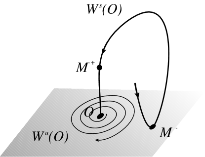
Figure 2: Geometry of the homoclinic orbit to a type $(1,2)$ saddle-focus for the map $\tilde{g}_{0}$ under assumptions (A^′)-(C^′).

As in the case of the type $(2,1)$ saddle-focus, we consider a three-parameter family $\tilde{g}_{\tilde{\varepsilon}}$ where $\tilde{\varepsilon}=(\tilde{\mu},P_{\tilde{\varepsilon}}-1,\psi-\psi_{0})$. We suppose here that $\tilde{\mu}$ is a splitting parameter, $P_{\tilde{\varepsilon}}=|\lambda(\tilde{\varepsilon})\gamma(\tilde{\varepsilon})^{2}|$ and $\lambda(0)=\lambda_{0},\gamma(0)=\gamma_{0}$.

Theorem 3.

Let $\tilde{g}_{\tilde{\varepsilon}}$ be the three-parameter general family defined above. Then, in any neighborhood of $\tilde{\varepsilon}=0$ there exist infinitely many open domains, $\tilde{\Delta}_{k}$, such that the first return map $\tilde{g}^{k}_{\tilde{\varepsilon}}$ takes the form

$$\begin{array}[]{l}\bar{X}=Y+o(1)_{k\to+\infty},\\ \bar{Y}=Z+o(1)_{k\to+\infty},\\ \bar{Z}=M_{1}+BX+M_{2}Z-Y^{2}+o(1)_{k\to+\infty},\\ \end{array}$$ (5)

where $(X,Y,Z)$ are rescaled coordinates and the domains of definition of the new coordinates and the parameters $(M_{1},M_{2},B)$ are arbitrarily large and cover, as $k\to\infty$, all finite values. Furthermore, the Jacobian, $B$, is positive or negative depending on the orientability of the map $\tilde{g}^{k}_{\varepsilon}$.The terms denoted $o(1)$ are functions (of the coordinates and parameters) that tend to zero as $k\to+\infty$ along with all derivatives up to order $r-2$.

Proof.

The proof immediate from Th. 2. Indeed, the inverse $\tilde{g}_{0}^{-1}$ is, evidently, a diffeomorphism satisfying the original conditions (A–(C). Thus, the map (4) is, in this case, the rescaled map for the inverse first return map $\tilde{g}_{\tilde{\varepsilon}}^{-k}$. The last can be be easily written in form (5), as we show explicitly below. ∎

The inverse of (1) is of interest in any case. Since (1) has the constant Jacobian $B$ it is invertible whenever $B\neq 0$. This inverse is

$$\begin{split}\bar{y}&=x,\;\;\bar{z}=y\;,\\ \bar{x}&=\frac{1}{B}(-M_{1}+z-M_{2}y+y^{2})\;.\end{split}$$

This map can be rewritten in the “standard” form of [LM98], if we define new variables $(x^{new},y^{new},z^{new})=B^{-1}(z,y,x)$ and new parameters

$$M_{1}^{new}=\frac{M_{1}}{B^{2}}\;,\;M_{2}^{new}=-\frac{M_{2}}{B},\;B^{new}=\frac{1}{B}\;,$$

then the resulting map has precisely the form (2). As we stated above map is well-known in homoclinic dynamics: it was found to be the rescaled first return map for four-dimensional diffeomorphisms that have a quadratic homoclinic tangency to a saddle-focus fixed point with two pairs of complex conjugate leading multipliers [GTS93],[GST96],[GST03].

The dynamics of each of the maps (1) and (2) is extremely rich. However, for the volume-contracting case, we note that these maps demonstrate distinct types of stable dynamics. For example, (1) gives rise to attractors similar to those of the Lorenz system, as we will see in §6. However, (2) need not have attractors of this “wild” type, although certainly, a “Lorenz repeller” will be present.

Nevertheless, we can expect existence of “extremely small” Lorenz-type attractors in (2) by the following argument. As we will see in §6, the map (2) can have a fixed point with multipliers $(+1,e^{i\omega},e^{-i\omega})$ at certain values of its parameters. The flow normal form near this point can have a homoclinic loop to a saddle-focus and, thus, (2) can have a fixed point $O$ with multipliers $(\gamma,\lambda e^{i\tilde{\omega}},\lambda e^{-i\tilde{\omega}})$, where $0<\lambda<1<\gamma$ and $\lambda^{2}\gamma=1$, such that the manifolds $W^{s}(O)$ and $W^{u}(O)$ will have a (quadratic) homoclinic tangency. Consequently, we can apply Th. 2 to this situation giving immediately the promised “extremely small” attractors.

Nevertheless, as it is shown in [GOST05] the Lorenz-type wild-hyperbolic attractor for (1) can be quite big and were observed to have a large basin. The proof of existence of big, globally attracting wild-hyperbolic attractors in map (2) is still open problem.

Finally, we consider the more general structure of polynomial diffeomorphisms of ${\mathbb{R}}^{3}$. As we remarked in the introduction, the 3D Hénon maps (1) and (2) have the form of (3) when $B=1$. As we will shown in §7, this result has the following generalization;

Theorem 4.

Let $f:{\mathbb{R}}^{3}\to{\mathbb{R}}^{3}$ be a quadratic diffeomorphism with a quadratic inverse and constant Jacobian $\det Df(x,y,z)=B$. Then, after an affine coordinate transformation $f$ can be written in the form (3) or else the dynamics of $f$ is trivial.

Note that both of the maps (1) and (2) fall into this classification. The classification of the dynamics of the trivial cases can be done from the normal forms (43) that will be obtained in §7.

3 Local and global maps

We begin the proof of Th. 1 by constructing a local map $T_{0}$, valid in a neighborhood $U_{0}$ of the fixed point $O$, that simplifies the description of the local unstable $W^{u}_{loc}(O)=W^{u}(O)\cap U_{0}$ and local stable $W^{s}_{loc}(O)=W^{s}(O)\cap U$ manifolds of $O$. Then we obtain a global map $T_{1}$ that takes a neighborhood of a point on $W^{u}_{loc}(O)$ to a neighborhood of a point of $W^{s}_{loc}(O)$.

By [GS93],[SSTC98], one can introduce $C^{r-1}$ coordinates $(x,y)=(x_{1},x_{2},y)$ in a neighborhood $U$ of the fixed point $O$ such that the local map $T_{0}(\varepsilon)\equiv g_{\varepsilon|U_{0}}$ can be written, for small enough $\varepsilon$, in the form

$$T_{0}:\begin{array}[]{lll}\bar{x}&=&\lambda R_{\varphi}x+\xi(x,y)\\ \bar{y}&=&\gamma y+\eta(x,y)\end{array}$$ (6)

where

$$R_{\varphi}=\begin{pmatrix}\cos\varphi&-\sin\varphi\\ \sin\varphi&\cos\varphi\end{pmatrix}$$ (7)

is the rotation by angle $\varphi$, and

$$\|\xi\|={\cal O}(\|x\|^{2}y)\;,\;\mbox{and}\;\eta={\cal O}(\|x\|y^{2})\;.$$ (8)

Here the coefficients, $\lambda,\varphi$, and $\gamma$ as well as $\xi$ and $\eta$ depend (smoothly) on the parameters $\varepsilon$. The form (6) will be called the main normal form; it is very convenient for calculations. In particular, the local stable and unstable manifolds of $O$ are $W^{s}_{loc}=\{(x,0)\}$ and $W^{u}_{loc}=\{(0,y)\}$ in the neighborhood $U$.

When $\varepsilon=0$, choose a homoclinic point $M^{-}=(0,0,y^{-})\in W^{u}_{loc}$ on the homoclinic orbit $\Gamma_{0}$ and a corresponding point $M^{+}=(x_{1}^{+},x_{2}^{+},0)\in W^{s}_{loc}$ that is an image of $M^{-}$: $M^{+}=g_{0}^{n_{0}}(M^{-})$ for some $n_{0}>0$, recall Fig. 1. Let $\Pi^{+}$ and $\Pi^{-}$ be some small neighborhoods of the points $M^{+}$ and $M^{-}$. The global map $T_{1}(\varepsilon)\equiv{g_{\varepsilon}^{n_{0}}}_{|\Pi^{-}}:\Pi^{-}\to\Pi^{+}$ is well defined for small enough $\varepsilon$, and can be written in the coordinates of (6) as

$$T_{1}:\begin{array}[]{ccl}\bar{x}-x^{+}&=&Ax+b(y-y^{-})+{\cal O}(\|x\|^{2}+|y-y^{-}|^{2}),\\ \bar{y}&=&y^{+}(\varepsilon)+c^{T}x+d(y-y^{-})^{2}+{\cal O}(\|x\|^{2}+\|x\||y-y^{-}|+|y-y^{-}|^{3}),\end{array}$$ (9)

where the $2\times 2$ matrix $A$, the vectors $x^{+}$, $b$, and $c$, the coefficients $y^{+}$ and $d$, and the higher order terms all depend smoothly on $\varepsilon$. We noted especially the dependence of the coefficient $y^{+}(\varepsilon)$ that will become the splitting parameter for the manifolds $W^{s}$ and $W^{u}$ near the homoclinic point $M^{+}$. As discussed in the previous section, we therefore denote it by

$$\mu=y^{+}(\varepsilon)$$ (10)

and consider as the first of the governing parameters.

The assumption (C) that the tangency between $W^{u}$ and $W^{s}$ is quadratic implies that

$$d\neq 0\;.$$ (11)

In addition, since $g_{0}$ is assumed to be a diffeomorphism, and since the Jacobian

$$DT_{1}(M^{-})=\begin{pmatrix}A&b\\ {c^{T}}&0\end{pmatrix}\;,$$ (12)

then we must have $\|b\|\neq 0$.

Indeed if $b_{2}(\varepsilon)$ is not identically zero, then one can use the linear coordinate change,

$$(x_{new},y_{new})=(R_{\vartheta}x,y)\;,$$ (13)

where $R_{\vartheta}$, (7), is a rotation by an angle $\vartheta(\varepsilon)$, to transform the map (9) to a new map of the same form such that the vector $b$ becomes

$$b^{T}=(b_{1},0)\;.$$ (14)

Here the new matrix $A$, point $x^{+}$, and vector $c$ are modified from the corresponding coefficients in the original (9).

Now the nonvanishing of the determinant of the Jacobian (12) implies that

$$J_{1}\equiv\det DT_{1}(M^{-})=b_{1}(a_{21}c_{2}-a_{22}c_{1})\neq 0\;.$$ (15)

One of merits of the main normal form (6) is that the iterations $T_{0}^{k}:U_{0}\to U_{0}$ for any $k$ can be calculated quite easily, namely, in a form close to the form when $T_{0}$ is linear. In particular for the linear case we have

$$x_{k}=\lambda^{k}R_{k\varphi}x_{0}\;,\quad y_{0}=\gamma^{-k}y_{k}\;.$$

This is the so-called cross-form of map $T_{0}^{k}$. We can write $T_{0}^{k}$ in an analogous cross-form when $T_{0}$ is in the form (6)

Lemma 5.

For any positive integer $k$ and for any sufficiently small $\varepsilon$ the map $T_{0}^{k}(\varepsilon):\;(x_{0},y_{0})\;\to\;(x_{k},y_{k})$ can be written in the cross-form

$$\begin{split}x_{k}&=\lambda^{k}R_{k\varphi}x_{0}+\lambda^{2k}\xi_{k}(x_{0},y_{k},\varepsilon)\;,\\ y_{0}&=\gamma^{-k}y_{k}+\lambda^{k}\gamma^{-k}\eta_{k}(x_{0},y_{k},\varepsilon)\;,\end{split}$$ (16)

where the vector $\xi_{k}$ and the function $\eta_{k}$ are uniformly bounded along with all derivatives up to order $(r-2)$. In addition, all of the derivatives of order $(r-1)$ for the functions $x_{k}$ and $y_{0}$ tend to $0$ as $k\rightarrow\infty$ .

Proof.

Let $(x_{i},y_{i})\in U\;,\;i=0,...,k,$ denote the orbit: $(x_{i},y_{i})=T_{0}(x_{i-1},y_{i-1})$. Then it is easy to see that the $j^{\mbox{th}}$ iterate of (6) is

$$\begin{split}x_{j}&=\lambda^{j}R_{j\varphi}x_{0}+\sum\limits_{s=0}^{j-1}\lambda^{j-s-1}R_{(j-s-1)\varphi}\xi(x_{s},y_{s},\varepsilon)\;,\\ y_{j}&=\;\gamma^{j-k}y_{k}-\sum\limits_{s=j}^{k-1}\gamma^{j-s-1}\eta(x_{s},y_{s},\varepsilon)\;.\end{split}$$ (17)

The solution of (17) for any given sufficiently small $x_{0},y_{k}$ and large $k$ (the so-called boundary value problem) can be found by successive approximations [AS73] if the zeroth approximation is taken as the corresponding solution of the linear problem. Using the fact that $|\lambda\gamma|>1$, we obtain the following estimates

$$\begin{array}[]{l}\|x_{k}-\lambda^{k}R_{k\varphi}x_{0}\|\leq L\sum\limits_{s=0}^{k-1}\lambda^{k-s-1}\lambda^{2s}|\gamma|^{s-k}\leq\tilde{L}\lambda^{2k},\\ |y_{0}-\gamma^{-k}y_{k}|\leq L\sum\limits_{s=0}^{k-1}|\gamma|^{-s-1}\lambda^{s}|\gamma|^{2s-2k}\leq\tilde{L}\lambda^{k}|\gamma|^{-k},\end{array}$$

where $L$ and $\tilde{L}$ are some positive constants estimating the norms for derivatives of the functions $\xi$ and $\eta$ in the domain $U$, from (6). These inequalities evidently imply the desired result for the map. Estimates for the derivatives can be found analogously. General results of this form for near saddle fixed point were given in [GS93],[SSTC98]. Here we give sharper estimates that apply in this particular case. ∎

4 Rescaled first return map: Proof of Th. 1

The main task of this section is to obtain an analytical form for the first return map for diffeomorphisms of the family $g_{\varepsilon}$ to a neighborhood of the homoclinic point $M^{+}$. To construct this map we first find an image of the local map $T_{0}$ for which $T_{0}^{k}(\Pi^{+})\cap\Pi^{-}\neq\emptyset$. This will be true for each $k\geq\bar{k}$ where $\bar{k}$ is some sufficiently large integer. For each such $k$ there are strips $\sigma_{k}^{+}\in\Pi^{+}$ and $\sigma^{-}_{k}\subset\Pi^{-}$ such that $T_{0}(\sigma_{k}^{+})=\sigma_{k}^{-}$. A first return map is obtained by composing $T_{0}^{k}$ with the global map $T_{1}:\Pi^{-}\rightarrow\Pi^{+}$, to obtain a map on a neighborhood of $M^{+}$, recall Fig. 1. Thus the first return map will be of the form

$$T_{k}\equiv T_{1}T_{0}^{k}\;,$$

Under the global map $T_{1}$ the strip $\sigma_{k}^{+}$ is transformed into three-dimensional horse-shaped region $T_{1}(\sigma_{k}^{+})$ that has non-empty intersection with $\sigma_{k}^{+}$ when $\varepsilon$ is small enough. Thus, the map $T_{k}$ is a generalized, three-dimensional, horseshoe map. We will show that these horseshoe maps can possess rich dynamics; for example, they can Lorenz-like, wild-hyperbolic strange attractors. The goal is the prove the following lemma:

Lemma 6 (Rescaling Lemma.).

For any sufficiently large $k$ such that

$$\begin{array}[]{l}A_{21}(k\varphi)\equiv a_{21}\cos k\varphi+a_{22}\sin k\varphi\neq 0\end{array}$$ (18)

the first return map $T_{k}$ can be brought, by means of an affine transformation of coordinates, to the following form

$$\begin{array}[]{l}\bar{Y}=Z+{\cal O}(\lambda^{k})\;,\\ \bar{X}=Y+{\cal O}(\lambda^{k}+|\lambda\gamma|^{-k})\;,\\ \bar{Z}=M_{1}-Z^{2}+b_{1}\lambda\gamma^{k}(c_{1}\cos k\varphi+c_{2}\sin k\varphi+\nu_{k}^{1})Y\\ +b_{1}A_{21}\lambda^{2k}\gamma^{k}(c_{2}\cos k\varphi-c_{1}\sin k\varphi+\nu_{k}^{2})X+{\cal O}(\lambda^{k})\;,\end{array}$$ (19)

where $\nu_{k}^{1,2}={\cal O}(\lambda^{k})$ are some coefficients,

$$\begin{array}[]{l}M_{1}=-d\gamma^{2k}[\mu-\gamma^{-k}y^{-}+\lambda^{k}\left(\cos k\varphi(c_{1}x_{1}^{+}c_{2}x_{2}^{+})+\sin k\varphi(c_{2}x_{1}^{+}-c_{2}x_{2}^{+})\right)+{\cal O}(\lambda^{2k})].\end{array}$$ (20)

Also, in (19) the ${\cal O}$-terms have the indicated asymptotic behavior for all derivatives up to order $(r-2)$.

Proof.

Using formulas (9), (16) and conditions (10) and (14) we can write the first return map $T_{k}\equiv T_{1}T_{0}^{k}$ in the form

$$\begin{array}[]{rll}\bar{x}_{1}&=&x_{1}^{+}+\lambda^{k}(e_{11}x_{1}+e_{12}x_{2})+b_{1}(y-y^{-})+\alpha_{1},\\ \bar{x}_{2}&=&x_{2}^{+}+\lambda^{k}(e_{21}x_{1}+e_{22}x_{2})+\alpha_{2},\\ \gamma^{-k}\bar{y}+\lambda^{k}\gamma^{-k}\eta_{k}(\bar{x},\bar{y},\varepsilon)&=&\mu+\lambda^{k}(c_{1}\cos k\varphi+c_{2}\sin k\varphi)x_{1}+\\ &&\lambda^{k}(c_{2}\cos k\varphi-c_{1}\sin k\varphi)x_{2}+d(y-y^{-})^{2}+\alpha_{3},\end{array}$$ (21)

where the $2\times 2$ matrix $E=AR_{k\varphi}$ and

$$\begin{array}[]{l}\alpha_{1,2}={\cal O}(\lambda^{2k}\|x\|+\lambda^{k}\|x\||y-y^{-}|+(y-y^{-})^{2}),\\ \alpha_{3}={\cal O}(\lambda^{2k}\|x\|+\lambda^{k}\|x\||y-y^{-}|+|y-y^{-}|^{3}).\end{array}$$

Introduce new coordinates

$$x_{new}=x-x^{+}+\beta_{k}^{1},\;y_{new}=y-y^{+}\beta_{k}^{2},$$

where $\beta_{k}={\cal O}(\lambda^{k})$, in order to eliminate the affine terms in the first two equations and the term linear in $y$ in the third equation of (21). Then, the map (21) is rewritten as

$$\begin{array}[]{l}\bar{x}_{1}=e_{11}\lambda^{k}x_{1}+e_{12}\lambda^{k}x_{2}+by+{\cal O}(\lambda^{2k}\|x\|+\lambda^{k}\|x\|\|y\|+\|y\|^{2}),\\ \bar{x}_{2}=e_{21}\lambda^{k}x_{1}+e_{22}\lambda^{k}x_{2}+{\cal O}(\lambda^{2k}\|x\|+\lambda^{k}\|x\|\|y\|+\|y\|^{2}),\\ \bar{y}+\lambda^{k}{\cal O}(\|\bar{x}\|+\|\bar{y}\|)=M+d\gamma^{k}y^{2}+\\ +\lambda^{k}\gamma^{k}(c_{1}\cos k\varphi+c_{2}\sin k\varphi+{\cal O}(\lambda^{k}))x_{1}+\lambda^{k}\gamma^{k}(c_{2}\cos k\varphi-c_{1}\sin k\varphi+{\cal O}(\lambda^{k}))x_{2}+\\ +\gamma^{k}{\cal O}(\lambda^{2k}\|x\|^{2}+\lambda^{k}\|x\|\|y\|+\|y\|^{3}),\end{array}$$ (22)

where $d_{new}=d+{\cal O}(\lambda^{k})$ and

$$\begin{array}[]{rlr}M&=&\gamma^{k}[\mu-\gamma^{-k}y^{-}+\lambda^{k}\left(\cos k\varphi(c_{1}x_{1}^{+}c_{2}x_{2}^{+})+\sin k\varphi(c_{2}x_{1}^{+}-c_{2}x_{2}^{+})\right)+{\cal O}(\lambda^{2k})].\end{array}$$ (23)

Next, we rescale the map (22) introducing new coordinates (X,Y,Z) defined through

$$x_{1}=-\frac{b_{1}}{d}\gamma^{-k}Y,\;\;x_{2}=-\frac{b_{1}A_{21}}{d}\lambda^{k}\gamma^{-k}X,\;\;y=-\frac{1}{d}\gamma^{-k}Z,$$ (24)

where we suppose that values of $\varphi$ are such that (18) holds. Then, map (22) is rewritten in the new coordinates in form (19). ∎

Now theorem 1 easily follows from this lemma. Indeed, we have only to indicate those domains $\Delta_{k}$ of the initial parameters where the coefficients in the third equation of (19) are finite. Denote the coefficient of the third equation of (19) in front of $Y$ as $M_{2}$, i.e.

$$\begin{array}[]{l}M_{2}\equiv b_{1}\lambda^{k}\gamma^{k}(c_{1}\cos k\varphi+c_{2}\sin k\varphi+\nu_{k}^{1}).\end{array}$$ (25)

Since $|\gamma|>1$ and $|\lambda\gamma|>1$, the coefficients $M_{1}$ and $M_{2}$ can take arbitrary finite values when varying parameters $\mu$ (for $M_{1}$) and $\varphi$ (for $M_{2}$), see formulas (20) and (25). Moreover, the finiteness of $M_{2}$ means that the corresponding values of the trigonometrical term $c_{1}\cos k\varphi+c_{2}\sin k\varphi$ are asymptotically small and, in any case, do not exceed $|\lambda\gamma|^{-k}$ in order. For such values of $\varphi$, we obtain

$$\begin{array}[]{l}c_{2}\cos k\varphi-c_{1}\sin k\varphi=\pm\sqrt{c_{1}^{2}+c_{2}^{2}}(1+...),\\ \displaystyle A_{21}\equiv a_{21}\cos k\varphi+a_{22}\sin k\varphi=\pm\frac{a_{21}c_{2}-a_{22}c_{1}}{\sqrt{c_{1}^{2}+c_{2}^{2}}}(1+...)\end{array}$$ (26)

Thus, by (15), $A_{21}\neq 0$ in this case. Denote as $B$ the coefficient in front of $X_{2}$ from the third equation of (19). By virtue of (26) and (15) we have

$$\begin{array}[]{l}B=b_{1}(a_{21}c_{2}-a_{22}c_{1})\lambda^{2k}\gamma^{k}(1+...)=J_{1}\lambda^{2k}\gamma^{k}(1+...).\end{array}$$ (27)

Since $|\lambda^{2}\gamma|=1$ at $\varepsilon=0$, it follows from (27) that $B$ can take (when $k$ is large) any arbitrary finite value (positive or negative depending on the sign of $J_{1}\lambda^{2k}\gamma^{k}$) as the value of the Jacobian $\lambda^{2}\gamma$ of the local map $T_{0}$ varies. This completes the proof of theorem 1.

Remarks

1. We noted that at least three parameters must be used to study bifurcations of a homoclinic orbit for a three-dimensional saddle-focus. The governing parameters that we use are $\varepsilon_{1}=\mu$ corresponding to the splitting distance between the stable and unstable manifolds, the phase $\varepsilon_{2}=\varphi-\varphi_{0}$ of the focus multiplier, and the Jacobian $\varepsilon_{3}=|\lambda^{2}\gamma|-1$ of the saddle-focus.

2. If the map $g_{0}$ is exactly volume preserving, i.e., $\det Dg_{0}\equiv 1$, then the resulting map (19) is as well, i.e. $B\equiv 1$. Such maps were studied in [LM98]. Moreover, Th. 2 implies that there are nearby maps (by unfolding the parameter $B$ to make the map volume contracting) that have strange attractors.

5 Local Bifurcations of 3D Hénon maps

In this section we will study the dynamics of the 3D Hénon map (1) and prove Th. 2. The dynamics can be complex, especially when $|B|$ is close to one, essentially because when $|B|=1$ the map has, for certain values of the parameters, fixed points with three multipliers are on the unit circle. It is well known that bifurcations of such points can lead to appearance of homoclinic tangencies, invariant circles, and even strange attractors (as $|B|$ decreases below one) or repellers (as $|B|$ increases above one) [Shi81],[SST93].

We are interested primarily in the stable dynamics of the map (1), i.e., in characterizing its attractors. One way to find attractors with complex dynamics is to study the local normal forms that arise near fixed points that have three multipliers that are $\pm 1$. We follow here the analysis of [SST93] where local normal forms of the equilibrium of a flow with three zero eigenvalues and with additional symmetries were analyzed and conditions for the existence of strange attractors were given. One of the most interesting of their results is that Lorenz attractors can appear by local bifurcations of an equilibrium with three zero eigenvalues when there is a reflection symmetry through the origin [Shi81],[SST93],[PST98]. These results can be applied to the local bifurcation analysis of (1) when the fixed points has multipliers $(+1,-1,-1)$.

As is true for the general volume-preserving quadratic diffeomorphism of Lomelí and Meiss [LM98], the 3D Hénon map (1) has at most two fixed points on the diagonal:

$$\begin{split}P_{\pm}&=(z_{\pm}^{*},z_{\pm}^{*},z_{\pm}^{*})\;,\\ z_{\pm}^{*}&=\frac{1}{2}\left({-1+B+M_{2}}\pm\sqrt{\Delta}\right)\;,\end{split}$$ (28)

providing that the discriminant, $\Delta$, is nonnegative,

$$\Delta\equiv(M_{2}+B-1)^{2}+4M_{1}\geq 0\;.$$ (29)

The primary bifurcations of these fixed points occur when they have multipliers on the unit circle. These bifurcations are easily determined using the characteristic polynomial of the Jacobian of (1),

$$p(\lambda)=\lambda^{3}+2z\lambda^{2}-M_{2}\lambda-B\;.$$

The first codimension-one case corresponds to a single multiplier one, where $p(1)=2z^{*}+1-B-M_{2}=0$, or equivalently to the surface where $\Delta$ vanishes:

$$L^{sn}\;:\;\;M_{1}=-\frac{1}{4}(M_{2}+B-1)^{2}\;.\\$$ (30)

This is simply a saddle-node bifurcation that creates the pair of fixed points (28) in the domain $\Delta>0$. Similarly, a period-doubling bifurcation occurs when there is a multiplier $-1$, i.e., where $p(-1)=2z^{*}-1-B+M_{2}=0$, or equivalently for $1-M_{2}=\pm\frac{1}{2}\sqrt{\Delta}$, which gives

$$L^{pd}\;:\;\;M_{1}=\frac{1}{4}(M_{2}-1-B)(3M_{2}-3+B)\;.\\$$ (31)

Note that this bifurcation occurs for the point $P_{+}$ when $M_{2}<1$, and for the point $P_{-}$ when $M_{2}>1$.

The final codimension-one bifurcation corresponds to the Hopf bifurcation when pair of multipliers is on the unit circle, $\lambda=e^{\pm i\varphi}$, so that

$$p(\lambda)=\lambda^{3}-(B+2\cos\varphi)\lambda^{2}+(1+2B\cos\varphi)\lambda-B\;,$$

or equivalently on the surface

$$L^{\varphi}\;:\;\;\left\{\begin{array}[]{l}M_{1}=(\cos\varphi+\frac{1}{2}B)\left((1-2B)\cos\varphi+\frac{3}{2}B-2\right),\\ M_{2}=-1-2B\cos\varphi\;.\\ \end{array}\right.$$ (32)

Here we have written the equation for the surface $L^{\varphi}$ in parametric form using the phase $0<\varphi<\pi$. When $B<1$, this bifurcation only occurs for the fixed point $P_{+}$.

There are three codimension-two curves in the $(M_{1},M_{2},B)$ parameter space. The Hopf surface, $L^{h}$ terminates at $L^{sn}$ when the multipliers are $(B,1,1)$ along the curve $(M_{1},M_{2})=(\frac{1}{4}(B+2)^{2},-2B-1)$. It also terminates on $L^{pd}$ where the multipliers are $(B,-1,-1)$ along the curve $(M_{1},M_{2})=(\frac{1}{4}(B-2)(7B-6),2B-1)$. Finally, the period-doubling and saddle-node curves are tangent when the multipliers are $(-B,-1,1)$ on the curve $(M_{1},M_{2})=(-\frac{1}{4}B^{2},1)$.

The bifurcation surfaces are most easily viewed in two-dimensional slices through constant $B$ planes. An example of the resulting bifurcation curves are shown when $B=0.6$ in Fig. 3 and Fig. 4. Note that $P_{+}$ is stable inside the curvilinear triangle bounded by $L^{sn}$, $L^{pd}$ and $L^{\varphi}$, when $B<1$. The second fixed point, $P_{-}$, is never stable when $B<1$.

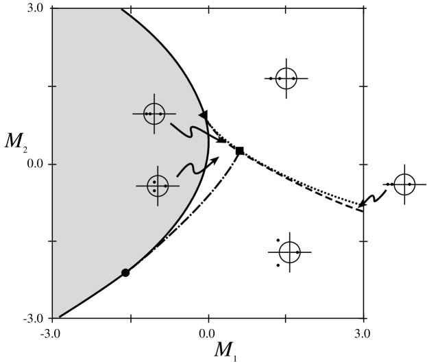
Figure 3: Bifurcation curves of the map (1) for the fixed point $P_{+}$ when $B=0.6$. Fixed points do not exist in the shaded region. The solid curve is the saddle-node $L^{sn}$, the dotted curve is the period doubling, $L^{pd}$, and dot-dash curve is the Hopf bifurcation, $L^{\varphi}$. The fourth curve (dashed) corresponds to the existence of a double eigenvalue. There are five corresponding regions, and a representative configuration of the multipliers in the complex-$\lambda$-plane is shown for each. The codimension-two bifurcations are shown as the “square” (period-doubling-Hopf), “triangle” (saddle-node-period doubling) and “‘circle” (saddle-node-Hopf) points.

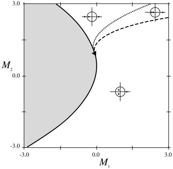
Figure 4: Bifurcation curves of the map (2) in for the fixed point $P_{-}$ when $B=0.6$. The curves have the same meaning as in Fig. 3. For this fixed point there is no Hopf bifurcation.

A similar analysis can be used to derive the bifurcation surfaces for the map (2). Indeed, the formula for the fixed points, and consequently the saddle-node surface is the same as for (1). The period-doubling and Hopf surfaces are slightly modified. An example of a slice through these surfaces for $B=0.6$ is shown in Fig. 5 and Fig. 6.

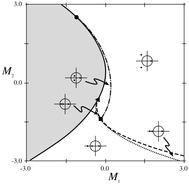
Figure 5: Bifurcation curves of the map (2) for the fixed point $P_{+}$ when $B=0.6$. The curves have the same meaning as in Fig. 3.

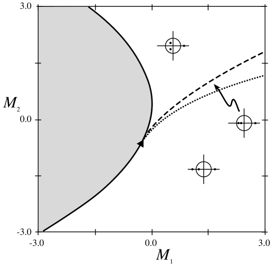
Figure 6: Bifurcation curves of the map (1) in for the fixed point $P_{-}$ when $B=0.6$. The curves have the same meaning as in Fig. 3. For this fixed point there is no Hopf bifurcation.

6 Wild-hyperbolic Lorenz attractors: Proof of Th. 2

We will now focus on the point $P_{+}$ and expand around the codimension-three bifurcation point where the multipliers are $(-1,-1,1)$, that is about the point $(M_{1},M_{2},B)=(-\frac{1}{4},1,1)$ where $z^{*}=1/2$. Note that on the parameter slice $B=1$, the Hopf curve (32) coincides with the saddle-node curve (30) so that there is no Hopf bifurcation. Moreover the codimension-two points in Fig. 3 corresponding to the multipliers $(-1,-1,B)$ (square) and $(-1,1,B)$ (triangle) collide at the codimension-three point. Otherwise the bifurcation diagram for $P_{+}$ looks similar the slice in the figure.

Our goal is to prove Th. 2. This can be done with the aid of the following lemma.

Lemma 7.

In a region of the parameters $(M_{1},M_{2},B)$ near the point $(-1/4,1,1)$ the second iterate of (1) in some neighborhood of $P_{+}$ is approximately the time-one map of the the three-dimensional flow

$$\begin{array}[]{l}\dot{x}=y\;,\\ \dot{y}=x(1-z)-\lambda y\;,\\ \dot{z}=-\alpha z+x^{2}\;,\end{array}$$ (33)

up to arbitrary small correction terms. Moreover the coordinates $(x,y,z)$ and parameters $\lambda$ and $\alpha$ can take arbitrary finite values.

Proof.

Shifting coordinates $x\to x-z_{+},y\to y-z_{+},z\to z-z_{+}$ brings map (1) to the form

$$\begin{split}\bar{x}=y,\;\;\bar{y}=z,\;\;\bar{z}=Bx+M_{2}y-2z_{+}z-z^{2}\end{split}$$ (34)

Introduce new (small) parameters $\varepsilon_{1},\varepsilon_{2},\varepsilon_{3}$ by the following formulas

$$\varepsilon_{1}=1-B,\;\varepsilon_{2}=1-M_{2},\;\varepsilon_{3}=2z_{+}-1.$$

Note that

$$\varepsilon_{1}>0,\;\varepsilon_{1}+\varepsilon_{2}+\varepsilon_{3}=\sqrt{\Delta}>0.$$

The first inequality means that $B<1$, and the second is fulfilled automatically when the fixed points exists, e.g. to the right of the $L^{sn}$ curve in Fig. 3. We have also the following relation

$$1+4M_{1}=\varepsilon_{3}^{2}+2(1+\varepsilon_{3})(\varepsilon_{1}+\varepsilon_{2})$$

between the new parameters and the parameter $M_{1}$. Next, we bring map (34) to the following form

$$\begin{array}[]{l}\bar{u}_{1}=-u_{1}+u_{2},\\ \displaystyle\bar{u}_{2}=\alpha_{1}u_{1}+(-1+\alpha_{2})u_{2}+u_{1}u_{3}-\frac{3}{2}u_{2}u_{3}+{\cal O}(\|u\|^{3}),\\ \displaystyle\bar{u}_{3}=(1+\alpha_{3})u_{3}-\frac{1}{4}u_{1}^{2}-\frac{1}{4}u_{3}^{2}+{\cal O}(\|u\|^{3}),\end{array}$$ (35)

where

$$2\alpha_{1}=\varepsilon_{1}-\varepsilon_{2}+\varepsilon_{3},\>\,4\alpha_{2}=\varepsilon_{1}+\varepsilon_{2}-3\varepsilon_{3},\>\,4\alpha_{3}=-(\varepsilon_{1}+\varepsilon_{2}+\varepsilon_{3}).$$

Note that the Jacobian of the map (35) is close to the Jordan normal form for the multipliers $(-1,-1,1)$ when $\alpha_{1},\alpha_{2},\alpha_{3}$ are small. The first equation of (35) does not contain any high order terms, and in the second and third components, we take into account only quadratic terms. Moreover, these quadratic terms have been further simplified by standard normal form analysis, so that only the resonant ones remain.

The second power of the map (35) can be embedded into a flow. Namely, using the Picard iteration procedure (of the second order), we can see that the map (35) coincides, up to terms of order ${\cal O}(\|u\|^{3})$, with the time-one map of the following flow

$$\begin{array}[]{l}\displaystyle\dot{u}_{1}=-2u_{2}-u_{1}u_{3}+\frac{5}{6}u_{2}u_{3}\\ \displaystyle\dot{u}_{2}=\beta_{1}u_{1}-\beta_{2}u_{2}-2u_{1}u_{3}+2u_{2}u_{3}\\ \displaystyle\dot{u}_{3}=\beta_{3}u_{3}-\frac{1}{2}u_{1}^{2}-\frac{1}{12}u_{2}^{2}-\frac{1}{2}u_{3}^{2}-\frac{1}{2}u_{1}u_{2}.\\ \end{array}$$ (36)

After a smooth change of coordinates of the form

$$v_{1}=u_{1},\;v_{2}=\dot{u}_{1},\;v_{3}=u_{3}+{\cal O}(\|u\|^{2})\;,$$

equations (36) are written as follows

$$\begin{array}[]{l}\dot{v}_{1}=v_{2}\\ \dot{v}_{2}=\bar{\mu}v_{1}-\bar{\lambda}v_{2}-av_{1}v_{3}-a_{1}v_{2}v_{3}\\ \dot{v}_{3}=-\bar{\alpha}+v_{3}^{2}+b(v_{1}^{2}+v_{2}^{2}),\end{array}$$ (37)

where

$$a=8,\>\,a_{1}=2,\>\,b=\frac{1}{4},\>\,\bar{\mu}=-\varepsilon_{1}-3\varepsilon_{2}-\varepsilon_{3},\\ \ \displaystyle\bar{\lambda}=\frac{\varepsilon_{1}+3\varepsilon_{2}-3\varepsilon_{3}}{2},\>\,\bar{\alpha}=\frac{(\varepsilon_{1}+\varepsilon_{2}+\varepsilon_{3})^{2}}{16}.$$

Flow (37) is the same that was considered [SST93] and, in our case we have also that $ab>0$. Then, we can introduce new time $\tau$ and new rescaled coordinates $(x,y,z)$, by formulas

$$\tau=st,\;\;{\rm where}\;\;s^{2}=\bar{\mu}+a\sqrt{\bar{\alpha}}=\varepsilon_{1}-\varepsilon_{2}+\varepsilon_{3},$$ (38)

$$v_{1}\to x\sqrt{\frac{s^{3}}{ab}},\>\,v_{2}\to y\tau\sqrt{\frac{s^{3}}{ab}},\>\,v_{3}\to-\sqrt{\bar{\alpha}}+\frac{s^{2}}{a}z,\>\,$$ (39)

such that system (37) is reduced to the following one

$$\begin{array}[]{l}\dot{x}=y,\\ \dot{y}=x(1-z)-\lambda y+{\cal O}(s),\\ \dot{z}=-\alpha z+x^{2}+{\cal O}(s),\end{array}$$ (40)

where

$$\begin{array}[]{l}\displaystyle\alpha=\frac{2\sqrt{\bar{\alpha}}}{\tau}=\frac{\varepsilon_{1}+\varepsilon_{2}+\varepsilon_{3}}{2\sqrt{\varepsilon_{1}-\varepsilon_{2}+\varepsilon_{3}}},\;\;\lambda=\frac{\bar{\lambda}}{\tau}=\frac{\varepsilon_{1}+3\varepsilon_{2}-3\varepsilon_{3}}{2\sqrt{\varepsilon_{1}-\varepsilon_{2}+\varepsilon_{3}}}.\end{array}$$ (41)

Since values of $s$ can be arbitrarily small, it implies that the rescaled coordinates $(x,y,z)$ and new parameters $\lambda$ and $\alpha$ can take arbitrarily finite values. ∎

Note that if we omit the ${\cal O}(s)$ terms in the system (40), we obtain system (33), which is the well-known, Shimizu-Morioka model. This system was intensively studied in [Shi86],[Shi93] where, in particular, the existence of the Lorenz attractor was proved for some domain of the parameters. For example, the domain of the existence of the Lorenz attractor in Shimizu-Morioka model is known to be contained in a rectangle $0.7<\lambda<1.5,\>\,0.1<\alpha<0.6$ ([SST93], fig. 13). Using this fact we can pointed out the following boundaries of values of the parameters $(\varepsilon_{1},\varepsilon_{2},\varepsilon_{3})$:

$$\begin{array}[]{l}\varepsilon_{1}>0\;,\\ \varepsilon_{1}+\varepsilon_{2}+\varepsilon_{3}>0\;,\\ \varepsilon_{1}-\varepsilon_{2}+\varepsilon_{3}>0\;,\\ \displaystyle 0.7<\frac{\varepsilon_{1}+3\varepsilon_{2}-3\varepsilon_{3}}{2\sqrt{\varepsilon_{1}-\varepsilon_{2}+\varepsilon_{3}}}<1.5\;,\\ \displaystyle 0.1<\frac{\varepsilon_{1}+\varepsilon_{2}+\varepsilon_{3}}{2\sqrt{\varepsilon_{1}-\varepsilon_{2}+\varepsilon_{3}}}<0.6\;,\end{array}$$ (42)

(and, respectively, of the parameters $(M_{1},M_{2},B)$) such that in the corresponding domain of the initial parameters $(M_{1},M_{2},B)$ our 3D Hénon map has a wild-hyperbolic Lorenz-type attractor. This completes the proof of the main theorem.
 

7 Quadratic Volume-Preserving Mappings: Proof of Th. 4

Suppose that $f:{\mathbb{R}}^{3}\rightarrow{\mathbb{R}}^{3}$ is a quadratic Cremona map, i.e., is a diffeomorphism with constant Jacobian $\det(Df)=B$. Then it is easy to see that without loss of generality we can write it in the form

$$f=S\circ L\circ(id+Q)\;.$$

where $S(x,y,z)=(B^{1/3}x,B^{1/3}y,B^{1/3}z)$ is the diagonal scaling map with $\det(S)=B$, $L$ is an affine volume-preserving map, $Q$ is a vector of quadratic forms so that the map $x+Q(x)$ is a volume-preserving quadratic shear [LM98].

As in Th. 4 we now assume that the map $f$ has a polynomial inverse (i.e., it is an element of the affine Cremona group) and that the inverse is also a quadratic map. The same property then will also hold for the volume-preserving map $g=S^{-1}\circ f$. It was shown in [LM98] that maps of the form $g$ can be transformed, by an affine change of variables, to one of the three following forms:

$$\begin{split}g_{1}(x,y,z)&=(y,z,M_{1}+M_{2}z+M_{3}y+x+q(y,z))\;,\\ g_{2}(x,y,z)&=(x_{0}+\frac{1}{M_{1}}x,y_{0}-M_{1}z,z_{0}+M_{2}z+y+q(x,z))\;,\\ g_{3}(x,y,z)&=(x_{0}+y+M_{1}x,y_{0}-\frac{1}{M_{2}}x,z_{0}+M_{2}z+q(x,y))\;,\end{split}$$

where $q(x,y)=ax^{2}+bxy+cy^{2}$ is a scalar quadratic form.

Consequently $g=A\circ g_{i}\circ A^{-1}$ for some affine transformation $A$, and $i=1$, $2$, or $3$. Using the same transformation on $f$ gives

$$\tilde{f}=A^{-1}\circ f\circ A=(A^{-1}\circ S\circ A)\circ g_{i}\;.$$

But the scaling map $S$ commutes with $A$, so

$$\tilde{f}=S\circ g_{i}\;.$$

Finally we can apply an additional scaling transformation to the variables and parameters to transform $\tilde{f}$ to one of the three forms

$$\begin{split}\tilde{f}_{1}(x,y,z)&=(y,z,M_{1}+M_{2}z+M_{3}y+Bx+q(y,z))\;,\\ \tilde{f}_{2}(x,y,z)&=(x_{0}+\frac{1}{M_{1}}x,y_{0}-M_{1}z,z_{0}+M_{2}z+By+q(x,z))\;,\\ \tilde{f}_{3}(x,y,z)&=(x_{0}+y+M_{1}x,y_{0}-\frac{1}{M_{2}}x,z_{0}+BM_{2}z+q(x,y))\;,\end{split}$$ (43)

where the parameters have been rescaled.

The dynamics of $\tilde{f}_{2}$ and $\tilde{f}_{3}$ are trivial. Indeed for $\tilde{f}_{2}$ the $x$ dynamics decouples from the remaining dynamics, and for $\tilde{f}_{3}$ the $(x,y)$ dynamics is linear and decouples from the $z$ dynamics.

Thus the only dynamically interesting case is $\tilde{f}_{1}$. Since this map is the same as (3), we have proved Th. 4.

An example of this analysis consider the ACT-map (Arneodo-Coullet-Tresser map) which was introduced by Arneodo, Coullet and Tresser in their study of strange attractors in a family of differential equations on ${\mathbb{R}}^{3}$ with homoclinic points of Shilnikov type [Du85].

$$\begin{array}[]{l}\bar{x}=ax-b(y-z),\\ \bar{y}=bx+a(y-z),\\ \bar{z}=cx-dx^{k}+ez,\end{array}$$ (44)

where $a,b,c,d,e$ are real parameters with $J=e(a^{2}+b^{2})\neq 0$, $bd\neq 0$, and $k>1$ an integer. The ACT-map always has a fixed point at the origin. Nevertheless, when $k=2$ it is a quadratic family with a quadratic inverse, so it follows from Th. 4 that it is affinely conjugate to (3) with $M_{1}=0$.

To see this explicitly define new coordinates using the transformation

$$X=\frac{ax+by}{a^{2}+b^{2}}\;,\;Y=x\;,\;Z=ax-b(y-z)\;,$$

then, the map is rewritten as

$$\begin{array}[]{l}\bar{X}=Y,\\ \bar{Y}=Z,\\ \bar{Z}=BX+S_{1}Y+S_{2}Z-bdY^{k}\end{array}$$

where where $B=e(a^{2}+b^{2}),S_{1}=-(a^{2}+b^{2}+cb+2ae),S_{2}=2a+e$. For the case $k=2$ we can rescale the coordinates by a factor $(bd)^{-1}$ to set the coefficient of $Y^{2}$ to one. Thus the map is written in the promised form (3).

Note that if we do one additional transformation and shift the variables by $S_{1}/2$ we can also obtain the standard form (2). Here we define $M_{1}=\frac{1}{4}S_{1}(2B+2S_{2}+S_{1}-2)$, and $M_{2}=S_{2}$. The inequality

$$\Delta=(1-B-M_{2})^{2}+4M_{1}=(B+S_{1}+S_{2}-1)^{2}\geq 0$$

holds guaranteeing the existence of a fixed point for the map.

8 Conclusions

We have seen that many phenomena in the dynamics of three-dimensional Hénon maps are markedly different from the possible phenomena predicted by our knowledge of two-dimensional dynamics. Primarily, we have seen these new phenomena when the Jacobian, $B$, is close to $\pm 1$. Two natural problems appear here, regarding the understanding of bifurcation scenarios that lead to chaotic three-dimensional dynamics. The first is to understand “how 2D dynamics is transformed into 3D dynamics” upon the variation of $B$ from values near zero to those close to $\pm 1$. The second problem—which is, in a sense, the inverse of the first one—is to understand “how 3D volume-preserving dynamics is transformed into dissipative (and chaotic) dynamics” as $B$ moves away from $\pm 1$. In the current paper (and also in [GOST05]), some partial results related to the second problem have been obtained; however, the first problem is—as of yet—unstudied.

However, our analysis implies that these global problems have no unified, qualitative solution. One general conclusion is that the stable dynamics of the Hénon maps of the first and second kind, (1) and (2), have unmistakably different characters. The bifurcations in (1) and (2) both lead eventually to the formation of three-dimensional versions of Smale horseshoes. However, these have different characters: the horseshoes of (1) contain type $(2,1)$ saddles of, while those of (2) contain type $(1,2)$ saddles. Thus, a third global problem appears: to understand “how the character of the attractors changes as one changes type of nonlinearity in 3D Hénon families.” In this case, it seems that using the family (3) with the parameters $(a,b,c)$ determining the type of nonlinearity may be very profitable.

While the problems posed above are of general interest, there are also many partial problems relating directly to the dynamics of quadratic maps. Some of these may also be solved in the the near future:

1. Does the Hénon map of the second kind, (2), have a large scale, wild-hyperbolic attractor?

2. What are the dynamical properties of the local normal form for (2) near fixed points with three unit multipliers?

   This is related to the ”reverse-Shimitsu-Marioka” system since (2) is the inverse of (1). Thus we will obtain the model (33), with $t$ replaced by $-t$. Consequently, the question is to determine the properties of the stable dynamics of this system.

3. What are main bifurcations scenarios the 3D Hénon map (1) that lead from simple dynamics to a wild-hyperbolic, Lorenz attractor?

   There are two distinct, but useful approaches: (a) to fix $B$ and consider the corresponding two-parameter family; (b) to consider $B$ as the main governing parameter and to move for given values of $(M_{1},M_{2})$ from small values of $B$ to values close to $\pm 1$.

4. What role is played by the codimension-two bifurcations (recall §5) in the formation of attracting invariant sets?

   The analysis of codimension-one bifurcations alone gives us only a representation of the main hyperbolic elements of the dynamics. A detail analysis of codimension-three bifurcations (as in §5) allows us to find in local normal forms (using the flow embedding approach) and verify the existence of small, wild-hyperbolic attractors. Analogous methods can be applied to the study of codimension-two bifurcations. We believe that this approach will provide an understanding of principal mechanisms for the creation of wild-hyperbolic attractors.

In summary, three-dimensional Hénon maps have an abundance of new dynamical behavior which, it seems, has an important place in the theory of multidimensional dynamics as whole. We believe that they form a natural direction for a program of investigation similar to the well developed programs in one and two-dimensional dynamics. This is especially true since these maps cover (up to the affine conjugacy) all possible quadratic three-dimensional automorphisms.

References

- [ABS77] V.S. Afraimovich, V.V. Bykov, and L.P. Shilnikov. The origin and structure of the Lorenz attractor. Sov. Phys. Dokl., 22:253-255, 1977.
- [ABS82] V.S. Afraimovich, V.V. Bykov, and L.P. Shilnikov. On attracting structurally unstable limit sets of lorenz attractor type. Trans. Mosc. Math. Soc., 44:153–216, 1982.
- [AS73] V.S. Afaimovich and L.P. Shilnikov. On critical sets of Morse-Smale systems. Trans. Moscow Math. Soc., 28:179–212, 1973.
- [AS83] V.S. Aframovich and L.P. Shilnikov. Strange attractors and quasiattractors. Nonlinear Dynamics and Turbulence, pages 1–34, 1983.
- [Baz93] A. Bazzani. Normal form theory for volume preserving maps. Z. Angew. Math. Phys., 44(1):147–172, 1993.
- [DA96] A.J. Dragt and D.T. Abell. Symplectic maps and computation of orbits in particle accelerators. In Integration algorithms and classical mechanics (Toronto, ON, 1993), pages 59–85. Amer. Math. Soc., Providence, RI, 1996.
- [Du85] B.S. Du. Bifurcations of periodic points of some diffeomorphisms on . Nonlinear Analysis, Theory, Methods and Applications, 9:309–319, 1985.
- [Eng58] W. Engel. Ganze cremona-transformationen von prinzahlgrad in der ebene. Math. Ann., 136:319–325, 1958.
- [FM89] S. Friedland and J. Milnor. Dynamical properties of plane polynomial automorphisms. Ergod. Th. & Dyn. Systems, 9:67–99, 1989.
- [For96] F. Forstneric. Actions of and on complex manifolds. Mat. Zeit., 223:123–153, 1996.
- [Gon00] S.V. Gonchenko. Dynamics and moduli of -conjugacy of 4D-diffeomorphisms with a structurally unstable homoclinic orbit to a saddle-focus fixed point. Methods of Qualitative Theory of Differential Equations and Related Topics, 200:107–134, 2000. Amer. Math. Soc. Transl. Ser. 2 Amer. Math. Soc. Providence, RI.
- [GG00] S.V.Gonchenko, V.S.Gonchenko. On Andronov-Hopf bifurcations of two-dimensional diffeomorphisms with homoclinic tangencies. WIAS-preprint, Berlin, No.556 (2000), 27p.
- [GG04] S.V.Gonchenko, V.S.Gonchenko. On bifurcations of birth of closed invariant curves in the case of two-dimensional diffeomorphisms with homoclinic tangencies. Proc. Steklov Inst., 244:80–105, 2004.
- [GOST05] S.V. Gonchenko, I.I. Ovsyannikov, C. Simó, and D.V. Turaev. Three-dimensional Hénon-like maps and wild Lorenz–like attractors. Int. J. of Bifurcation and Chaos, 15(11), 2005.
- [GS72] N.K. Gavrilov and L.P. Shilnikov. On three-dimensional dynamical systems close to systems with a structurally unstable homoclinic curve. Part I, Math. USSR Sb., 17:467–485, 1972.
- [GS73] N.K. Gavrilov and L.P. Shilnikov. On three-dimensional dynamical systems close to systems with a structurally unstable homoclinic curve. Part II, Math. USSR Sb., 19:139–156, 1973.
- [GS93] S.V. Gonchenko and L.P. Shilnikov. On moduli of systems with a structurally unstable homoclinic Poincaré curve. Russian Acad. Sci. Izv. Math., 41(3):417–445, 1993.
- [GST96] S.V. Gonchenko, L.P. Shilnikov, and D.V. Turaev. Dynamical phenomena in systems with structurally unstable Poincaré homoclinic orbits. Chaos, 6(1):15–31, 1996.
- [GST03] S.V. Gonchenko, L.P. Shilnikov, and D.V. Turaev. On dynamical properties of diffeomorphisms with homoclinic tangencies. Contemprary Mathematics and Its Applications, 7:92–118, 2003. English version is in: WIAS-preprint No.795, Berlin 2002.
- [GTS91] S.V. Gonchenko, D.V. Turaev, and L.P. Shilnikov. On models with a structurally unstable homoclinic Poincaré curve. Methods in Qualitative Theory and Bifurcation Theory (Russian), pages 36–61, 1991.
- [GTS93] S.V. Gonchenko, D.V. Turaev, and L.P. Shilnikov. Dynamical phenomena in multidimensional systems with a structurally unstable homoclinic poincaré curve. Russian Acad. Sci. Dokl. Math, 47(3):410–415, 1993.
- [GTS99] S.V.Gonchenko, D.V.Turaev and L.P.Shilnikov. Homoclinic tangencies of an arbitrary order in Newhouse domains. in Itogi Nauki Tekh., Ser. Sovrem. Mat. Prilozh., 67:69-128, 1999. [English translation in J.Math. Sci., 105:1738-1778, 2001].
- [GW79] J. Guckenheimer and R. F. Williams. Structural stability of Lorenz attractors. Inst. Hautes Études Sci. Publ. Math., 50:59–72, 1979.
- [H7́6] M. Hénon. A two-dimensional mapping with a strange attractor. Comm. Math. Phys., 50:69–77, 1976.
- [Jun42] H.W.E. Jung. Über ganze birationale Transformationen der Ebene. J. Reine Angew. Math., 184:161–174, 1942.
- [LLM99] K. E. Lenz, H. E. Lomelí, and J.D. Meiss. Quadratic volume preserving maps: an extension of a result of Moser. Regular and Chaotic Motion, 3:122–130, 1999.
- [LM98] H.E. Lomelí and J.D. Meiss. Quadratic volume preserving maps. Nonlinearity, 11:557–574, 1998.
- [MGBC96] C. Mira, L. Gardini, A. Barugolo, and J-C. Cathala. Chaotic dynamics in two-dimensional noninvertible maps, volume 20 of Nonlinear Science Series A. World Scientific, 1996.
- [Mos94] J.K. Moser. On quadratic symplectic mappings. Math. Zeitschrift, 216:417–430, 1994.
- [N79] S.Newhouse. The abundance of wild hyperbolic sets and non-smooth stable sets for diffeomorphisms. Publ. Math. IHES, 50:101-152, 1979.
- [PST98] V. Pisarevsky, A.L Shilnikov, and D.V. Turaev. Asymptotic normal forms for equilibria with a triplet of zero characteristic exponents in systems with symmetry. Regular and Chaotic Dynamics, 2:123–135, 1998.
- [Shi81] L.P. Shilnikov. The bifurcation theory and quasi-hyperbolic attractors. Uspehi Mat. Nauk, 36:240–241, 1981.
- [Shi86] A.L. Shilnikov. Bifurcation and chaos in the Marioka-Shimizu system. In Methods of qualitative theory of differential equations, pages 180–193. Gorky, 1986. English translation in Selecta Math. Soviet. 10 (1991), 105-117.
- [Shi93] A.L. Shilnikov. On bifurcations of the Lorenz attractor in the Shimuizu-Morioka model. Physica D, 62:338–346, 1993.
- [SST93] A.L. Shilnikov, L.P. Shilnikov, and D. V. Turaev. Normal forms and Lorenz attractors. Internat. J. Bifur. Chaos Appl. Sci. Engrg., 3(5):1123–1139, 1993.
- [SSTC98] L.P. Shilnikov, A.L. Shilnikov, D.V. Turaev, and L.O. Chua. Methods of qualitative theory in nonlinear dynamics, Part I. World Scientific, Singapore, 1998.
- [ST98] L.P. Shilnikov and D.V. Turaev. An example of a wild strange attractor Sb. Math., 189(2):137–160, 1998.
- [SU04] I.P. Shestakov and U.U. Umirbaev. The tame and the wild automorphisms of polynomial rings in three variables. J. Amer. Math. Soc., 17(1):197–227, 2004.
- [Tat01] J.C. Tatjer. Three dimensional dissipative diffeomorphisms with homoclinic tanjencies. Ergodic Theory Dynam. Systems, 21(1):249–302, 2001.
- [TLY86] L. Tedeschini-Lalli and J.A. Yorke. How often do simple dynamical processes have infinitely many coexisting sinks? Commun. Math. Phys., 106:635–657, 1986.
- [Tur03] D.V. Turaev. Polynomial approximations of symplectic dynamics and richness of chaos in non-hyperbolic area-preserving maps. Nonlinearity, 16:123–135, 2003.
- [TS05] D.V. Turaev and L.P.Shilnikov. The Lorenz attractor under a small periodic forcing. in preparation.