Statistics and geometry of passive scalars in turbulence

Abstract

We present direct numerical simulations (DNS) of the mixing of the passive scalar at modest Reynolds numbers ($10\leq R_{\lambda}\leq 42$) and Schmidt numbers larger than unity ($2\leq Sc\leq 32$). The simulations resolve below the Batchelor scale up to a factor of four. The advecting turbulence is homogeneous and isotropic, and maintained stationary by stochastic forcing at low wavenumbers. The passive scalar is rendered stationary by a mean scalar gradient in one direction. The relation between geometrical and statistical properties of scalar field and its gradients is examined. The Reynolds numbers and Schmidt numbers are not large enough for either the Kolmogorov scaling or the Batchelor scaling to develop and, not surprisingly, we find no fractal scaling of scalar level sets, or isosurfaces, in the intermediate viscous range. The area-to-volume ratio of isosurfaces reflects the nearly Gaussian statistics of the scalar fluctuations. The scalar flux across the isosurfaces, which is determined by the conditional probability density function (PDF) of the scalar gradient magnitude, has a stretched exponential distribution towards the tails. The PDF of the scalar dissipation departs distinctly, for both small and large amplitudes, from the lognormal distribution for all cases considered. The joint statistics of the scalar and its dissipation rate, and the mean conditional moment of the scalar dissipation, are studied as well. We examine the effects of coarse-graining on the probability density to simulate the effects of poor probe-resolution in measurements.

I Introduction

The mixing of passive scalars in the presence of turbulent motion is a subject of great theoretical and practical interest. Examples of its ubiquitous applications arise in reacting flows and combustion, mixing of salt and plankton in oceans and of pollutants in the atmosphere, as well as mixing of biological substances. Much experimental effort has thus been invested on mapping scalar fields in three dimensions, usually by reconstructing them from several planar cuts taken in quick succession in time; see Refs. 1 to 6 for work on turbulent liquid or air jets and Refs. 7 and 8 for work on diffusion flames. The Schmidt number $Sc=\nu/\kappa$ where $\nu$ is the kinematic viscosity of the advecting fluid and $\kappa$ is the scalar diffusivity, plays an important role in determining the nature of mixing batchelor . For the following, our focus will be on Schmidt numbers larger than unity.

The finest scales of the scalar are generally thought to be of the order of the Batchelor scale defined as $\eta_{B}=\eta/\sqrt{Sc}$ where $\eta$ is the Kolmogorov scale given by $\eta=\nu^{3/4}/\langle\epsilon\rangle$; $\epsilon$ is the local energy dissipation rate of turbulence, and the angular brackets indicate a suitable average. For a given flow, the Batchelor scale becomes smaller for larger $Sc$. Thus, the required resolution for large $Sc$, common in liquid flows, is hard to attain experimentally bilger04 .

With modern computers, it is possible to resolve scalar mixing in turbulence at high Schmidt numbers yeung01 ; yeung02 ; brethouwer03 ; schu03 ; watanabe04 . Schumacher et al. schu05 showed that it is sometimes necessary to resolve scales that are finer than $\eta_{B}$. Such fine resolutions are desired, for instance, for obtaining reliable results on the extreme fluctuations (both small and large) of scalar gradients and scalar dissipation rate. We resolve scales finer than the Batchelor scale by a factor of four. This fine resolution limits the ranges of $Sc$ and $R_{\lambda}$ examined, where $R_{\lambda}$ is the Taylor microscale Reynolds number. Nevertheless, we can study trends with $Sc$ and $R_{\lambda}$ in limited ranges of these parameters, with full three-dimensional field resolved extremely well. In particular, we consider relations between geometric and statistical properties of passive scalars and their spatial variations with respect to $Sc$ for a given turbulent flow, as well as those with the Reynolds number for a given $Sc$.

The paper is organized as follows. Section II briefly reports the numerical details and parameters. We consider the box-counting properties and area-to-volume ratio of the passive scalar isosurfaces in Sec. III, while Sec. IV considers the properties of the instantaneous scalar flux across isosurfaces. Section V presents an analysis of the statistics of scalar dissipation including conditional statistics. Conclusions and summary are presented in the final section.

II Numerical Simulations

We solve simultaneously the Navier-Stokes equations for an incompressible flow ${\bf u}({\bf x},t)$ and the advection-diffusion equation for the passive scalar field $\theta({\bf x},t)$ in box-type three-dimensional turbulence with the classical pseudo-spectral method that uses fast Fourier transformations and a 2/3 de-aliasing. The boundary conditions for the velocity and scalar field are both periodic. The simulation domain has a length of $2\pi$ in each coordinate direction and is resolved by an equidistant grid with $N^{3}$ points. The equations are

$$\frac{\partial{\bf u}}{\partial t}+({\bf u}\cdot{\bf\nabla}){\bf u} = -{\bf\nabla}p+\nu{\bf\nabla}^{2}{\bf u}+{\bf f}\,,$$ (1)

$${\bf\nabla}\cdot{\bf u} = 0\,,$$ (2)

$$\frac{\partial\theta}{\partial t}+({\bf u}\cdot{\bf\nabla})\theta = \kappa{\bf\nabla}^{2}\theta-u_{y}G\,.$$ (3)

Here, $p({\bf x},t)$ is the kinematic pressure field. The turbulence is sustained by a random force density ${\bf f}({\bf x},t)$ (see Vedula et al. yeung01 and Schumacher schu04 for details) and the scalar gradient is constant in the $y$ direction, i.e. ${\bf G}=(0,G,0)$ with $G=1$; $u_{y}$ is the turbulent velocity component in the direction $y$. The equations are integrated in time by a second-order predictor-corrector scheme. Parameters of the simulations and some statistical results are listed in Table 1. The spectral resolution exceeds the usual criterion of $k_{max}\eta_{B}\geq 1.5$ by a factor of about 4. A detailed comparison between these high-resolution data and those with the nominal resolution employed in most DNS studies was presented in Schumacher et al. schu05 . Their conclusion was that super-fine resolution would be needed to capture specific features of the scalar dissipation rate

$$\epsilon_{\theta}({\bf x},t)=\kappa({\bf\nabla}\theta({\bf x},t))^{2}\,,$$ (4)

such as the sheet-like structures in which the extreme events are found. We shall exploit the present fine resolution for just such purposes.

Run No.	1			2			3
$N$	512			1024			1024
$\nu$	0.0333			0.0133			0.005
$\langle\epsilon\rangle$	0.1			0.1			0.1
$u_{rms}$	0.394			0.483			0.486
$k_{m}\eta$	33.56			33.56			15.93
$R_{\lambda}$	10			24			42
$L$	1.018			0.920			0.758
$T_{av}/T_{E}$	9.1			1.2			1.1
$Sc$	2	8	32	2	8	32	32
$\theta_{rms}$	1.390	2.012	2.572	1.269	1.604	1.917	1.548
$\langle\epsilon_{\theta}\rangle$	0.330	0.391	0.420	0.307	0.345	0.372	0.306
$k_{m}\eta_{B}$	23.68	11.84	5.92	23.68	11.84	5.92	2.82
$L_{\theta}$	0.707	0.587	0.477	0.562	0.447	0.357	0.289

Table 1: List of parameters for the present DNS runs. $N$ is the number of grid points on each side of the computational cube, $\nu$ is the kinematic viscosity, $\langle\epsilon\rangle$ is the mean energy dissipation rate, $u_{rms}\equiv\langle u_{x}^{2}\rangle^{1/2}$ is the root-mean-square velocity fluctuation in $x$ direction, $k_{m}=\sqrt{2}N/3$ is the maximum wavenumber allowed in the simulations, $R_{\lambda}=\sqrt{15/(\nu\langle\epsilon\rangle)}\,\langle u_{x}^{2}\rangle$ is the Taylor microscale Reynolds number, $L$ is the integral scale of turbulence. Its magnitude is to be compared with the linear dimension of the box, which is $2\pi$ in all cases. $T_{av}$ is the statistical averaging time, to be compared here with the large-eddy turnover time defined as $T_{E}=\langle{\bf u}^{2}\rangle/2\langle\epsilon\rangle$; $Sc$ is the Schmidt number, $\theta_{rms}\equiv\langle\theta^{2}\rangle^{1/2}$ is the root-mean-square passive scalar fluctuation, $\langle\epsilon_{\theta}\rangle$ is the mean scalar dissipation rate and $L_{\theta}$ is the integral scale of the passive scalar. Both integral scales are calculated as in Ref. 44.

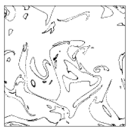
Figure 1: Two-dimensional instantaneous slice through the fluctuating passive scalar field $\theta({\bf x},t)$ for the level of $0.8\,\theta_{rms}$ (i.e., $X=0.8$). The side-length of the box (Run 2) is about 90$\eta$ and resolved with $N=1024$ in each coordinate direction. $R_{\lambda}=24$, $Sc=32$.

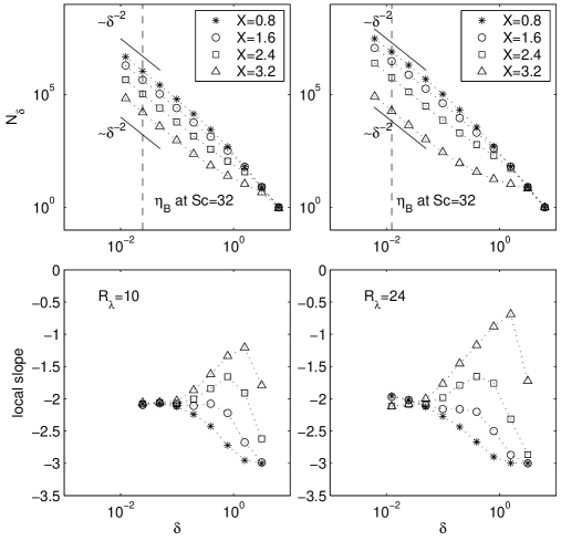
Figure 2: Three-dimensional box-counting data for scalar level sets $L_{X}$ as defined in (5) for $Sc=32$ and for $R_{\lambda}=10$ (left column) and $R_{\lambda}=24$ (right column). The values of $X$ are: asterisks, 0.8; circles, 1.6; squares, 2.4; triangles, 3.2. The vertical dashed lines in the upper panels show the corresponding values of $\eta_{B}$. Short solid lines mark the algebraic slope with $\delta^{-2}$ in the log-log plot. All the isosurfaces have a region with a common exponent of 2 at the smallest scales. The lower panels show the local slope $\mbox{d}\log(N_{\delta})/\mbox{d}\log(\delta)$ as a function of $\delta$. Symbols are as in the upper figures.

III Scalar isosurfaces

III.1 Box-counting dimension

It is well-known that, for Schmidt numbers exceeding unity, the passive scalar is filamented in structure and mixed by smooth flow in a continual stretch-twist-fold scenario Ott . An open point is whether the scalar contours accompanying such dynamics, when diffusion and external driving are included, generate fractal sets. Neither the inertial-convective range nor the viscous-convective Batchelor range obtains for the present moderate values of $R_{\lambda}$ and $Sc$, so it would be surprising if the fractal scaling is found. Nevertheless, the issue is worth a brief examination as a prelude to the study of area-to-volume ratio of scalar interfaces that follows in Sec. III B. If the surface is indeed a fractal, it is easy to write down the surface area in terms of its dimension and the cut-off scales terminating the scaling behavior sreeni .

Let us define the scalar level sets as

$$L_{X}=\{{\bf x}:X-\delta X\leq\theta({\bf x},t)/\theta_{rms}\leq X+\delta X\}\,,$$ (5)

where $X$ is the ratio of the chosen amplitude threshold to the root-mean-square value of the scalar, $\theta_{rms}$. Operationally, $\delta X$ is taken to be $2.5\%$ of $\theta_{rms}$ for each $(R_{\lambda},Sc)$. Figure 1 shows a level set of the scalar field around a value of $0.8\theta_{rms}$ for $Sc=32$ and $R_{\lambda}=24$. Similar pictures with different thresholds show that levels of high intensity are embedded within iso-levels of lower intensity. The iso-levels become increasingly disconnected with increasing intensity and become isolated islands embedded within an iso-contour of lower magnitude. This observation is consistent with mixing studies in a jet by Villermaux and Innocenti villermaux99 . In the box-counting procedure described, for example, in Falconer Falconer , one counts the number of cubes, $N_{\delta}$, of side-length $\delta$ that cover the level set $L_{X}$ completely. This procedure is repeated for various values of $\delta$. The box-counting dimension $D$ of a (fractal) level set is defined then as

$$D=-\lim_{\delta\to 0}\;\frac{\log N_{\delta}}{\log\delta}\,.$$ (6)

In practice, it is clear that one cannot apply the limit $\delta\to 0$ and one seeks an algebraic scaling, $N_{\delta}\sim\delta^{-D}$, in a finite range.

The upper two panels of Fig. 2 show the log-log plots resulting from box-counting for data sets of Runs 1 and 2 at $Sc=32$. A constant slope with exponent $D$ would give the box-counting dimension of the scalar level set. However, the local slope given by

$$D(\delta)=-\frac{\mbox{d}\log N_{\delta}}{\mbox{d}\log\delta}\,$$ (7)

varies continuously, as shown in the lower panels of Fig. 2. Though our simulations cover three orders of magnitude of scales, it is clear that no power-law scaling exists for reasons mentioned at the beginning of this section. The smallest few values of $\delta$ give a local slope of 2, for all $X$, which means that the level sets at those scales become smooth sheets. We interpret (the slightly) smaller slopes for intermediate scales of $\delta$ as arising from the disconnected shape of the iso-level sets. Indeed, this patchiness increases with the level $X$ thus giving a smaller magnitude of the local slope.

The conclusion from this study is that fractal behavior of the isolevel sets is not obtained in the range of $R_{\lambda}$ and $Sc$ considered here. We want to emphasize, however, that this finding has no bearing on the past experimental work as reported in Refs. 3, 4, 19 and 21. The differences such as may exist in these experimental studies require a separate discussion which lies outside the scope of this paper. We expect that the fractal property in the inertial-convective range requires high Reynolds numbers while that in the viscous-convective range requires high values of Schmidt and Reynolds numbers.

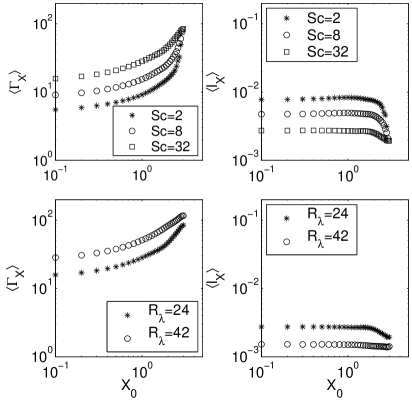
Figure 3: Left column: mean of the area-to-volume ratio $\langle\Gamma_{X}\rangle$ as a function of the isolevel $X$ in a log-log plot. Upper panel shows data for Run 2 at three different Schmidt numbers. Lower panel shows the quantity at $Sc=32$ for Runs 2 and 3. Right column: the corresponding mean thickness scale $\langle\ell_{X}\rangle$ as derived from Eq. (10).

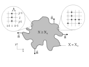
Figure 4: Sketch of the scalar gradient flux calculation across an passive scalar isosurface $X=X_{0}$. The illustration is for a two-dimensional case (but the data presented in the next figure are for the surface in three dimensions). Black points lie on the boundary whereas the gray points are the interior of $\tilde{L}_{X}$. The inner points are the volume that is used for $\Gamma_{X}$ (see Eq. (9)).

III.2 Area-to-volume ratio

Since we do not have fractal scaling for the ranges of parameters considered here, it is necessary to compute the area of isosurfaces directly. In reacting flows, a quantity of some importance is the ratio of the isosurface area content to the volume which encloses it pope88 . This ratio is numerically calculated as follows. We first define the set

$$\tilde{L}_{X}=\{{\bf x}:\theta({\bf x},t)/\theta_{rms}\geq X\}\,.$$ (8)

The set is computed for each snapshot separately and the results are averaged with respect to time subsequently. We mark all grid points that belong to $\tilde{L}_{X}$ by an indicator function $I_{ijk}\equiv 1$. For all other points, $I_{ijk}\equiv 0$. Here $i$, $j$, and $k$ denote the indices of the grid vertices running from 1 to $N$. All boundary points of the set $L_{X}$ have a number of nearest neighbors, $N_{ijk}$, that ranges from 1 to 5; the inner points of $\tilde{L}_{X}$ have 6 nearest neighbors. The number of inner points is denoted by $\overline{N}_{ijk}$. The area-to-volume ratio $\Gamma_{X}$ of the set $\tilde{L}_{X}$ is given by

$$\Gamma_{X}=\frac{A_{X}}{V_{X}}=\frac{1}{\overline{N}_{i,j,k}\Delta x}\sum_{(i,j,k)\in\tilde{L}_{X}}\,(6-N_{ijk})\,,$$ (9)

with grid spacing $\Delta x$, with $\overline{N}_{i,j,k}\neq 0$. The left column of Fig. 3 shows the average of the area-to-volume ratio, with $\langle\Gamma_{X}\rangle$ taken over several snapshots. Three trends are clear: first, the ratio grows with increasing $X$, which indicates a higher degree of disconnection of the isosurfaces. Second, the ratio is larger for larger Schmidt numbers. This is because mixing then occurs over ever finer scales whose contours are stretched and folded by the flow. Finally, a larger Reynolds number enables the scalar to be stirred more efficiently on all scales, yielding larger area-to-volume ratios with increasing Reynolds number.

We relate this geometric measure to statistical properties of the passive scalar fluctuations following ideas that were used in the slightly different context of interfacial dynamics for a turbulent jet aguirre04 . As is shown later (see Sec. V B), the scalar fluctuations are close to the Gaussian probability density function, $p(X)=1/\sqrt{2\pi}\,\exp(-X^{2}/2)$, with a slight sub-Gaussian behavior in the far tails. The average of the ratio $\langle\Gamma_{X}\rangle$ should therefore be related to $p(X)$. For $X=X_{0}$ we set

$$\langle\Gamma_{X_{0}}\rangle\,\langle\ell_{X_{0}}\rangle\simeq\frac{\exp(-X_{0}^{2}/2)\,\mbox{d}X_{0}}{\int_{X_{0}}^{\infty}\,\exp(-y^{2}/2)\,\mbox{d}y}=\frac{\exp(-X_{0}^{2}/2)\,\mbox{d}X_{0}}{\sqrt{\pi/2}\left[1-\mbox{erf}(X_{0}/\sqrt{2})\right]}\,,$$ (10)

where $\mbox{erf}(x)=(2/\sqrt{\pi})\int_{0}^{x}\,\exp(-y^{2})\,\mbox{d}y$ is the error function. For the following, we discuss results for values $X_{0}>0$, but everything holds for $X_{0}<0$ just the same way. The additional scale $\langle\ell_{X_{0}}\rangle$ on the left hand side of Eq. (10) has to appear for dimensional reasons since the right hand side is dimensionless.

The scale $\langle\ell_{X_{0}}\rangle$ is related to the surface-to-volume ratio $\Gamma$, and is small when the surface-to-volume ratio is large. Since $\Gamma$ becomes larger for “rougher” surfaces, the scale is a characteristic measure of the transition between smooth and rough isosurfaces, perhaps describing the average connectedness and regularity of the isosurface. We may thus call it the transition scale. It is a global average measure as well as $\Gamma$. Its trends with $Sc$ and $R_{\lambda}$ are shown in the right column of Fig. 3. The straight horizontal parts of $\langle\ell_{X}\rangle$ for $X\lesssim 2$ at fixed $Sc$ and $R_{\lambda}$ are the “geometric fingerprints” of the Gaussianity of the scalar fluctuations. Finally, we want to note that the relation (10) holds only for isosurfaces that are not fractal.

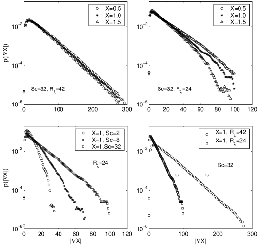
Figure 5: The probability density function of the magnitude of scalar gradient, $|{\bf\nabla}X|$, taken at iso-contour levels $X=X_{0}$. Upper left: The data are for Run 3, $Sc=32$, for three different levels: $X=0.5$ (open circle), $X=1.0$ (asterisk), $X=1.5$ (triangle). Upper right: The data are for Run 2, $Sc=32$, for three different levels: $X=0.5$ (open circle), $X=1.0$ (asterisk), and $X=1.5$ (triangle). Lower left: Schmidt number dependence of the flux. Data are for Run 2 at $X=1$: $Sc=2$ (circle), $Sc=8$ (asterisk), and $Sc=32$ (square). Lower right: Reynolds number dependence of the flux for $Sc=32$ and for $X=1$, with $R_{\lambda}=24$, Run 2 (square) and $R_{\lambda}=42$, Run 3 (circle). The vertical arrows (dashed for Run 2 and solid for Run 3) indicate $X/\eta_{B}$ with $X=1$.

IV Flux across scalar isosurfaces

One reason for the interest in the area of an isosurface is the flux across it. For example, in non-premixed turbulent combustion the isosurface of the stochiometric mixture fraction plays an important role and the variation of gradients across it are important for closure models pope88 ; bilger04 ; verwisch98 . This can be calculated by integrating the flux across all infinitesimal elements of the surface. Since the flux is proportional to the product of the area and the gradient of the concentration across it, it is necessary to know the gradient across each infinitesimal element of the surface. The gradient can itself be a highly fluctuating variable.

The present data allow the computation of gradients and fluxes across infinitesimal elements of isosurfaces. The (differential) flux across an infinitesimal area element $\mbox{d}A$ of an isosurface is given by

$$\mbox{d}\Phi(X_{0})=-{\bf\nabla}X|_{X=X_{0}}{\bf\cdot n}\,\mbox{d}A\,,$$ (11)

where ${\bf n}$ is the outward unit normal (see Fig. 4 for $X_{0}>0$).

The probability density function (PDF) of $\mbox{d}\Phi(X_{0})$ is then fully determined by the PDF of scalar gradient magnitude at the isolevel $X=X_{0}$

$$p(\mbox{d}\Phi(X_{0}))=p(-|{\bf\nabla}X|_{X=X_{0}}\,\mbox{d}A)\,.$$ (12)

Thus, the quantity of interest is a conditional PDF $p(|{\bf\nabla}X|\,|X=X_{0})$ which is calculated as follows. First, as in the preceding section, we mark all the grid points for which $\theta({\bf x},t)\geq X\theta_{rms}$ as active points; their grid sites are marked with $I_{i,j,k}\equiv 1$; for all other points, $I_{i,j,k}\equiv 0$. Gradients are calculated on $\partial\tilde{L}_{X}$ afterwards. Sparser grid resolutions would require a trilinear interpolation between the grid cells Kollmann1997 .

The result is plotted in Fig. 5. A stretched exponential behavior is observed for a large range of the PDF, with the tails decaying more rapidly for larger $X$. The PDFs suggests also that there is a considerable local variation of the flux across interfaces $X=X_{0}$. The fluctuations increase significantly with increase in $Sc$ as well as $R_{\lambda}$. For both Reynolds numbers, one can see low-probability instances whose gradients are of the order of $\theta_{rms}/\eta_{B}$. This particular gradient value is indicated in the lower right figure by the two vertical arrows.

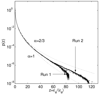
Figure 6: Log-linear plot of the probability density function of the scalar dissipation rate, normalized to the mean value. Data are for Run 1 and Run 2 at $Sc=32$. Fits to the data for $z\geq 10$ with the exponential term of (13) are also plotted and the corresponding exponents $\alpha$ are shown. The dashed line is the optimum of a least square fit resulting in $\alpha=0.86$.

Figure 7: Upper panel: Probability density function of $z=(\log(\epsilon_{\theta})-\langle\log(\epsilon_{\theta})\rangle)/\sigma$ with $\sigma=\sqrt{\langle(\log(\epsilon_{\theta}))^{2}\rangle-\langle\log(\epsilon_{\theta})\rangle^{2}}$. Data for Run 2, with $Sc=32$, are compared with the corresponding lognormal distribution having the same mean and standard deviation. Data in each panel are plotted as a solid line and the lognormal distribution as a dotted line. The inset shows the same data in a log-linear plot that highlights the tails. Deviations from lognormality are quite visible. Lower panel: Log-linear plots of the same type of data for three different Reynolds numbers and $Sc=32$.

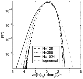
Figure 8: Log-linear plot of the PDF of the scalar dissipation rate at $Sc=32$ for Run 2. As in Fig. 7, solid line are the original data at a resolution of $N=1024$ and the dotted line is for the corresponding lognormal distribution. The analysis was repeated for the coarse-grained scalar dissipation field, and the dashed line shows the result of coarse-graining over $8^{3}$ cubes, giving an effective resolution of $N=128$; the dashed-dotted curve is for $4^{3}$ cubes with an effective resolution of $N=256$.

V Statistics of scalar dissipation rate

V.1 The PDF of the scalar dissipation rate

The scalar dissipation rate plays a central role in determining turbulent mixing. In combustion, for example, its properties enter fast chemistry models bilger76 , modelling of thin reactive layers called flamelets peters86 which are embedded and advected in the turbulent flow, and conditional-moment closures for the evolution of the mixture fraction in non-premixed cases klimenko99 .

With $p(|{\bf\nabla}\theta|)\sim\exp(-(C|{\bf\nabla}\theta|^{\alpha})$ for large $|{\bf\nabla}\theta|$, as was seen in the last section, we expect that the tails of the PDF of $\epsilon_{\theta}$ will have stretched exponential behavior given by

$$p(\epsilon_{\theta}>\langle\epsilon_{\theta}\rangle)=\frac{C_{1}}{\sqrt{\epsilon_{\theta}}}\,\exp\left(-C_{2}\epsilon_{\theta}^{\alpha/2}\right)\,,$$ (13)

where $C_{1}$ and $C_{2}$ are constants. Such statistics were derived analytically for scalar advection in smooth and white-in-time flows for the limit $Pe\to\infty$ and $\alpha=2/3$ was found Falkovich98 ; Gamba99 . In Fig. 6 we show the PDF of the scalar dissipation rate in a log-lin plot for Runs 1 and 2; Sc=32. In addition, we fit the exponential part of the formula (13) to the data for the range of $\epsilon_{\theta}>10\langle\epsilon_{\theta}\rangle$. The cases $\alpha=1$ (pure exponential) and $\alpha=2/3$ (corresponding to the theory in Refs. 29 and 30) bound both sets of data from below and above, respectively, with the optimal least-square fit (dashed line) corresponding to $\alpha=0.86$.

This form of the PDF departs clearly from log-normality. Figure 7 (upper panel) shows the PDF of $\epsilon_{\theta}$ for Run 2 (see Table 1). The linear scale reveals that the lognormal approximation is not particularly good near the core. The logarithmic scale (inset) shows that the tails depart from lognormality as well: low dissipation values show a fatter tail and high dissipation values fall short of the lognormal. These departures from lognormality are robust for all Reynolds and Schmidt numbers considered here: this is demonstrated in the lower panel of Fig. 7 where we plot the data for $Sc=32$ at the three Reynolds numbers $R_{\lambda}$=10, 24, and 42.

There has been much discussion in the literature about the lognormality or otherwise of scalar dissipation, and we might cite an early paper Sreenivasan and Antonia sreenivasan and a recent one by Su and Clemens su03 to illustrate experimental results and the discussions accompanying them. Often, measured deviations from lognormality are attributed to poor measurement resolution or to low Reynolds numbers or to noise in the experimental system.

In order to shed some light on how the PDFs depend on probe resolution in an experiment, we plot in Fig. 8 the PDFs that result when the statistics are taken over successively coarse-grained scalar dissipation fields. The coarse-graining scale does not produce a qualitatively different result on the right side of the distribution ($z>0$), for which the PDF remains sub-Gaussian for all cases. For negative $z$, there is probably a particular coarse-graining that may collapse the data on to the lognormal curve, but this coincidence would be accidental at best. On the effect of Reynolds number, we can only comment that the behavior is similar for both Reynolds numbers considered here. The double-precision calculations throughout this work keep the noise effects under control. We thus conclude that, while the PDF is roughly lognormal, the deviations from it are considerable.

V.2 The joint statistics of scalar and scalar dissipation

In Fig. 9 we show the joint PDF $p(\theta,\epsilon_{\theta})$ where $p(\theta,\epsilon_{\theta})\,\mbox{d}\theta\,\mbox{d}\epsilon_{\theta}$ is the probability of having the scalar dissipation rate between $\epsilon_{\theta}$ and $\epsilon_{\theta}+\mbox{d}\epsilon_{\theta}$ and the scalar fluctuation between $\theta$ and $\theta+\mbox{d}\theta$. The figure shows the joint PDF for two Reynolds numbers and $Sc=32$. The upper row of Fig. 9 shows iso-contours of $p(\theta,\epsilon_{\theta})$ which are equidistant in units of the logarithm to base 10. The joint PDF is wider with respect to the $\theta$-axis for the case of larger Reynolds number. This is due to the fact that the scalar field and the dissipation field acquire larger amplitudes with increasing $R_{\lambda}$. The lower panels show the scalar PDF calculated by integrating $p(\theta,\epsilon_{\theta})$ over $\epsilon_{\theta}$. We observe an almost Gaussian shape of $p(\theta)$ for both Reynolds numbers (as anticipated in Sec. III.B). Additionally, we have compared our results with the limiting shape for a scalar field PDF that was analytically predicted for advection in a random flow yakhot89 . The comparison is good only for small amplitudes of $\theta$.

A nearly Gaussian PDF for the scalar fluctuations is in agreement with a number of other studies at $Sc\lesssim 1$, such as heated grid turbulence mydlarski98 , isotropic turbulence with a mean scalar gradient overholt ; celani01 , a homogeneous shear flow with heating by a constant mean temperature gradient ferchichi . In our simulations, the fluctuations extend to approximately $\pm 4.5\theta_{rms}$ and the deviations in the tails are slightly sub-Gaussian. Exponential tails of the PDF, as found by Jayesh and Warhaft jayesh , were not observed for our range of parameters. It should be mentioned that they were also predicted analytically for a white-in-time smooth Gaussian flow by Shraiman and Siggia shraiman . Furthermore, exponential tails have been suggested to result from an aggregation process of elementary local straining motion events, and close-to-exponential tails have been observed in jets sufficiently far away from the nozzle exit villermaux03 .

Overholt and Pope overholt argued that the nearly Gaussian or slightly sub-Gaussian statistics may result from the limited size of the simulation box in relation to the integral scale. The ratio of our box size to the integral scale of the flow, $2\pi/L$, is about 6 to 8 (see Table 1); in terms of the integral scale of the passive scalar at the largest Schmidt number, the ratio $2\pi/L_{\theta}$ varies from 13 to 21. This is significantly larger than the corresponding scale ratios in the experiment of Jayesh and Warhaft. The available evidence thus suggests that the relative size of the box size to the integral scale is not responsible for the shape of the PDF. A plausible argument can be made that the ratio $L/L_{\theta}$ might be a more appropriate quantity. We have attempted to vary this ratio in the simulations, but the results are still not conclusive.

The average of the scalar dissipation rate conditioned on the relation $\theta({\bf x},t)=\psi$ is denoted by $\langle\epsilon_{\theta}|\theta=\psi\rangle$. The conditional average is defined by means of the conditional probability density function $p(\epsilon_{\theta}|\theta)$, as

$$\langle\epsilon_{\theta}|\theta=\psi\rangle=\int_{0}^{\infty}\,\mbox{d}\epsilon_{\theta}\,\epsilon_{\theta}\,p(\epsilon_{\theta}|\theta=\psi)\,.$$ (14)

The conditional probability density function can be expressed via the joint probability density function of having the scalar dissipation between $\epsilon_{\theta}$ and $\epsilon_{\theta}+\mbox{d}\epsilon_{\theta}$ and the scalar between $\theta$ and $\theta+\mbox{d}\theta$, so that

$$p(\epsilon_{\theta}|\theta=\psi)=\frac{p(\theta=\psi,\epsilon_{\theta})}{p(\theta=\psi)}\,.$$ (15)

Figure 10 shows the conditional moments for $Sc=2$ and 32. It is well known that the conditional moment is constant obrien if the scalar distribution is strictly Gaussian. As can be seen in Fig. 10 our numerical results confirm this prediction for scalar fluctuation levels of less than about three standard deviations. For larger scalar fluctuation levels, there is a considerable drop in the conditional expectation. This suggests a precipitous drop in $\epsilon_{\theta}$ for large values of $\theta$, in contrast, say, to the behavior of the energy dissipation field $\epsilon$ with respect to the velocity fluctuations krs-sd .

Experiments in inhomogeneous flows kailas show that the constancy of the conditional moment holds roughly on the centerline of turbulent jets and wakes. The behavior off-center is quite complex, and the boundary layer flows are intrinsically different.

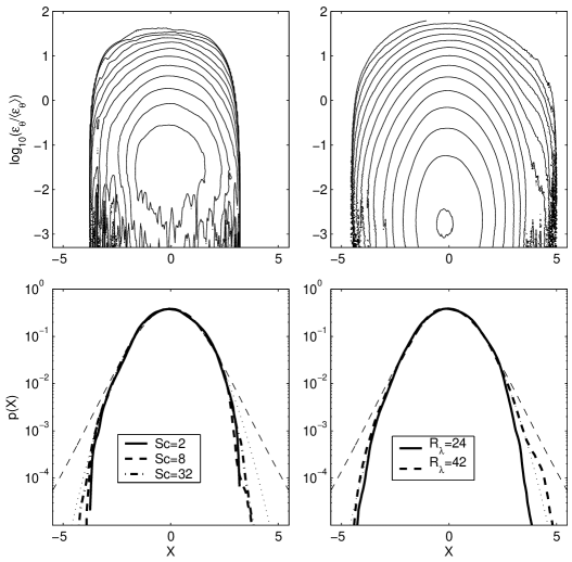
Figure 9: Upper row: Joint probability density function $p(\theta/\theta_{rms},\epsilon_{\theta}/\langle\epsilon_{\theta}\rangle)$ for the runs at $R_{\lambda}=24$ (left) and $R_{\lambda}=42$ (right), both for $Sc=32$. The iso-contour levels are equidistant in units of the logarithm to base 10, varying from $-6$ to 0.5 in steps of 0.5. The joint densities for large negative values of log$(\epsilon_{\theta})$ (i.e., scalar dissipation rates smaller than $10^{-3}\langle\epsilon_{\theta}\rangle$) are truncated for reasons of poor convergence. Lower row: scalar PDF for $R_{\lambda}=24$ and $Sc$ values indicated in the legend (left). The thin dashed line is a theoretical prediction for the scalar PDF, $p(X)=C/(1+kX^{2})^{1+1/2k}$, for advection in a random flow with fit parameters $C=0.4$, $k=0.08$, $X$ being $\theta/\theta_{rms}$ yakhot89 . The thin dotted line is a Gaussian distribution. Scalar PDF at $Sc=32$ for two different Reynolds numbers as indicated in the legend are shown in the right panel. Both thin lines are as in the lower left panel.

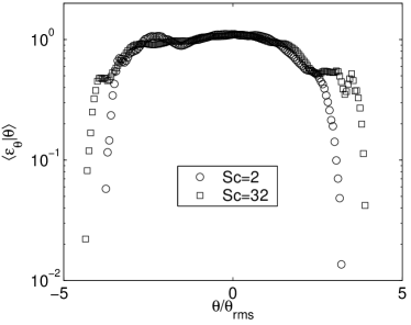
Figure 10: Mean conditional moment of the scalar dissipation rate for Schmidt numbers $Sc=2$ and 32. Data are for Run 2 in Table 1.

VI Summary and conclusions

We have studied numerically the dynamics of passive scalars advected in homogeneous isotropic turbulence for three Schmidt numbers $Sc>1$ and three Reynolds numbers, $R_{\lambda}$. These Reynolds and Schmidt numbers are moderate but comparable to those of many laboratory experiments on reacting flows. Usually, in such flows, neither the inertial range nor the viscous-convective range is well developed. The most important range of scales then belong to the so-called intermediate viscous range, which essentially pertain to the crossover between the inertial and viscous ranges of scales frisch91 ; schu05 . In this range, rough velocity filaments reach down into the viscous range below the Kolmogorov scale $\eta$ and stir the scalar. As reported in Ref. 16, the intermediate viscous range gets more extended with increasing Reynolds number. We have paid particular attention to the grid resolution of the simulations, which exceeds the nominal value by a factor of four, to ensure that the high intensity events of the scalars and their gradient fields are resolved well.

The first quantity considered is the area-to-volume ratio of isoscalar surfaces because of its fundamental relevance to reacting flows. For the Reynolds and Schmidt numbers considered here, the fractal scaling of isoscalar level sets is not obtained and so cannot be used to estimate the area-to-volume ratio. This ratio, computed here directly, increases with an increase in the passive scalar isolevel, the Schmidt number, and the Reynolds number, respectively. In detail, these increasing trends depend on the statistics of the scalar itself, which is found here to be nearly Gaussian.

We have defined a so-called transition scale $\langle\ell_{X}\rangle$ that becomes smaller with increasing surface-to-volume ratio of the isosurface corresponding to the scalar magnitude $X$ (normalized by the root-mean-square value). Quite understandably, the isosurface becomes ”rougher” and more disconnected with increasing $Sc$ and increasing Reynolds number, but is not dependent on $X$ itself—except when $X$ is large. The flat behavior of the scale $\langle\ell_{X}\rangle$ for $X\lesssim 2$ can be considered a geometric confirmation of the nearly Gaussian probability density function $p(X)$ of the scalar. For large $X$, there is a tendency for $\langle\ell_{X}\rangle$ to decrease with $X$, this being attributable to the sub-Gaussian behavior of $p(X)$ in the tail region. The flux across the interface is a strongly fluctuating quantity from one differential area element to another, and its distribution is closely exponential. The fluctuations increase rapidly with increase in $Sc$ as well as $R_{\lambda}$. Though with low probability, gradients of the order of magnitude $\theta_{rms}/\eta_{B}$ do occur in the scalar field. This clearly suggests the existence of sharp fronts accompanied by large jumps in the scalar concentration.

The scalar dissipation rate departs from lognormality more than previous measurements suggest. The reasons for close correspondence in previous data are not entirely clear, but it must be pointed out that very few data sets exist in which all three scalar gradient components that enter the scalar dissipation rate definition (see (Eq. 4)) were measured with adequate resolution and without the use of Taylor’s hypothesis. To consider if the closeness to lognormality observed previously was caused by poor resolution in measurements, we coarse-grained the data and replotted them. The coarse-grained data also display significant departures from lognormality. We thus conclude that the reasons for observed departures are more complex; they may also emphasize the lack of strict universality in the dissipation statistics.

The high spectral resolution in the present DNS allowed the evaluation of a conditional moment analysis as well. We have been able to confirm theoretical predictions that follow from nearly Gaussian fluctuations of the passive scalar field for $\theta<3\theta_{rms}$, say.

In summary, we have quantified various properties of the scalar isosurfaces for conditions that are typical of many laboratory experiments in reacting flows. Beside the connections between statistical and geometrical properties of scalars studied here, it is interesting to shed more light on the formation of characteristic scalar structures with respect to time, and to relate them to the underlying local flow properties for different Reynolds numbers. This can be a useful way of incorporating Reynolds number effects on mixing in the Batchelor regime and is part of the future work.

- (1) R.R. Prasad and K.R. Sreenivasan, “Quantitative three-dimensional imaging and the structure of passive scalar fields in fully turbulent flows,” J. Fluid Mech. 216, 1 (1990).
- (2) K.A. Buch, Jr. and W.J.A. Dahm, “Experimental study of the fine-scale structure of conserved scalar mixing in turbulent shear flows. Part 1. ,” J. Fluid Mech. 317, 21 (1996).
- (3) H.J. Catrakis and P.E. Dimotakis, “Scale distributions and fractal dimensions in turbulence,” Phys. Rev. Lett. 77, 3795 (1996).
- (4) E. Villermaux and C. Innocenti, “On the geometry of turbulent mixing,” J. Fluid Mech. 393, 123 (1999).
- (5) H.J. Catrakis, R.C. Aguirre and J. Ruiz-Plancarte,“Area-volume properties of fluid interfaces in turbulence: scale-local self-similarity and cumulative scale dependence,” J. Fluid Mech. 462, 245 (2002).
- (6) L.K. Su and N.T. Clemens,“The structure of fine-scale scalar mixing in gas-phase planar turbulent jets,” J. Fluid Mech. 488, 1 (2003).
- (7) S.H. Stårner, R.W. Bilger, K.M. Lyons, J.H. Frank and M.B. Long, “Conserved scalar measurements in turbulent-diffusion flames by a Raman and Rayleigh ribbon imaging method,” Combust. Flame 99, 347 (1994).
- (8) A.N. Karpetis and R.S. Barlow, “Measurements of scalar dissipation in a turbulent piloted methane/air jet flame,” Proc. Combust. Inst. 29, 1929 (2002).
- (9) G.K. Batchelor, “Small-scale variation of convected quantities like temperature in a turbulent fluid. Part 1. General discussion and the case of small conductivity,” J. Fluid Mech. 5, 113 (1959).
- (10) R.W. Bilger, “Some aspects of scalar dissipation,” Flow Turb. Combust. 72, 93 (2004).
- (11) P. Vedula, P.K. Yeung and R.O. Fox, “Dynamics of scalar dissipation in isotropic turbulence: a numerical and modelling study,” J. Fluid Mech. 433, 29 (2001).
- (12) P.K. Yeung, S. Xu and K.R. Sreenivasan, “Schmidt number effects on turbulent transport with uniform mean scalar gradient,” Phys. Fluids 14, 4178 (2002).
- (13) G. Brethouwer, J.C.R. Hunt and F.T.M. Nieuwstadt, “Micro-structure and Lagrangian statistics of the scalar field with a mean gradient in isotropic turbulence,” J. Fluid Mech. 474, 193 (2003).
- (14) J. Schumacher and K.R. Sreenivasan, “Geometric features of the mixing of passive scalars at high Schmidt numbers,” Phys. Rev. Lett. 91, 174501 (2003).
- (15) T. Watanabe and T. Gotoh, “Statistics of passive scalar in homogeneous turbulence,” New J. Phys. 6, 40 (2004).
- (16) J. Schumacher, K.R. Sreenivasan and P.K. Yeung, “Very fine structures in scalar mixing,” J. Fluid Mech. 531, 113 (2005).
- (17) J. Schumacher, “Relation between shear parameter and Reynolds number in statistically stationary shear flows,” Phys. Fluids 16, 3094 (2004).
- (18) E. Ott, Chaos in dynamical systems, Cambridge University Press, Cambridge, 2002.
- (19) K.R. Sreenivasan, R. Ramshankar and C. Meneveau, “Mixing, entrainment, and fractal dimension of interfaces in turbulent flows,” Proc. Roy. Soc. Lond. 421A, 79 (1989).
- (20) K.J. Falconer, The geometry of fractal sets, Cambridge University Press, Cambridge, 1985.
- (21) R.D. Frederiksen, W.J.A. Dahm, and D.R. Dowling, “Experimental assesment of fractal scale-similarity in turbulent flows. Part 1. One-dimensional intersections,” J. Fluid Mech. 327, 35 (1996).
- (22) S.B. Pope, “The evolution of surfaces in turbulence,” Int. J. Eng. Sci. 26, 445 (1988).
- (23) R. C. Aguirre and H. J. Catrakis, “Interfacial-fluid dynamics and the mixing efficiency of turbulent flows,” Phys. Fluids 16, 4746 (2004).
- (24) L. Verwisch and T. Poinsot, “Direct numerical simulation of non-premixed turbulent flames,” Annu. Rev. Fluid Mech. 30, 655 (1998).
- (25) W. Kollmann and J.J. Lienau, “Computation of topological and geometric properties of isosurfaces I: theory and numerical method,” Int. J. Comp. Fluid Dyn. 8, 83 (1997).
- (26) R.W. Bilger, “Turbulent jet diffusion flames,” Progr. Energy Combust. Sci. 1, 87 (1976).
- (27) N. Peters, “Laminar flamelet concepts in turbulent combustion,” Proc. Combust. Inst. 21, 1231 (1986).
- (28) A.Y. Klimenko and R.W. Bilger, “Conditional moment closure for turbulent combustion,” Progr. Energy Combust. Sci. 25, 595 (1999).
- (29) M. Chertkov, G. Falkovich and I. Kolokolov, “Intermittent dissipation of a passive scalar in turbulence,” Phys. Rev. Lett. 80, 2121 (1998).
- (30) A. Gamba and I. Kolokolov, “Dissipation statistics of a passive scalar in a multi-dimensional smooth flow,” J. Stat. Phys. 94, 759 (1999).
- (31) K.R. Sreenivasan, R.A. Antonia and H.Q. Dahn, “Temperature dissipation fluctuations in a turbulent boundary layer,” Phys. Fluids 20, 1238 (1977).
- (32) Y.G. Sinai and V. Yakhot, “Limiting probability distributions of a passive scalar in a random velocity field,” Phys. Rev. Lett. 63, 1962 (1989).
- (33) L. Mydlarski and Z. Warhaft, “Passive scalar statistics in high-Péclet number grid turbulence,” J. Fluid Mech. 358, 135 (1998).
- (34) M. R. Overholt and S. B. Pope, “Direct numerical simulation of a passive scalar with imposed mean gradient in isotropic turbulence,” Phys. Fluids 8, 3128 (1996).
- (35) A. Celani, A. Lanotte, A. Mazzino and M. Vergassola, “Fronts in passive scalar turbulence,” Phys. Fluids 13, 1768 (2001).
- (36) M. Ferchichi and S. Tavoularis, “Scalar probability density function and fine structure in uniformly sheared turbulence,” J. Fluid Mech. 461, 155 (2002).
- (37) Jayesh and Z. Warhaft, “Probability distribution of a passive scalar in grid-generated turbulence,” Phys. Rev. Lett. 67, 3503 (1991).
- (38) B. I. Shraiman and E. D. Siggia, “Lagrangian path integral and fluctuations in random flow,” Phys. Rev. E 49, 2912 (1994).
- (39) E. Villermaux and J. Duplat, “Mixing as an aggragation process,” Phys. Rev. Lett. 91, 184501 (2003).
- (40) F. Gao and E.E. O’Brien, “Joint probability density function of a scalar and its gradient in isotropic turbulence,” Phys. Fluids A 3, 1625 (1991).
- (41) K.R. Sreenivasan and B. Dhruva, “Is there scaling in high-Reynolds-number turbulence?” Prog. Theo. Phys. 130, 103 (1998).
- (42) P. Kailasnath, K.R. Sreenivasan and J.R. Saylor, “Conditional scalar dissipation rates in turbulent wakes, jets and boundary layers,” Phys. Fluids A5, 3207 (1993).
- (43) U. Frisch and M. Vergassola, “A prediction of the multifractal model: the intermediate dissipation range,” Europhys. Lett. 14, 439 (1991).
- (44) D.A. Donzis, P.K. Yeung, and K.R.Sreenivasan, “Scalar dissipation rate and dissipative anomaly in isotropic turbulence,” J. Fluid Mech. 532, 199 (2005).