Synchronization of Limit Sets

C.P. Li¹ and W.H. Deng^2,1

¹Department of Mathematics, Shanghai University, Shanghai 200444, China

²School of Mathematics and Statistics, Lanzhou University, Lanzhou 730000, China

In this Letter, we derive a sufficient condition of synchronizing limit sets (attractors and repellers) by using the linear feedback control technique proposed here. There examples are included. The numerical simulations and computer graphics show that our method work well.

Historically, the study of synchronization phenomena of dynamical systems has been an active topic in physics. In the 17th century, Huggens found two synchronization clocks, other early discovered examples, such as, wobbly bridges, the oscillating uniformly Josephson junctions, the synchronized lightning fireflies, synchronization of adjacent organ pipes, emerging coherence in chemical oscillators, etc [1].

In recent decades, the research on synchronization moved to chaotic systems. As we know, an essential characteristic of chaotic system is that its evolution sensitively depends on initial conditions, intuitionally, this intrinsically defy synchronization. But in 1990 Pecora and Carroll [2] pointed out that when we coupled two identical chaotic systems, the synchronization between them is possible. In the sequel, lots of methods and techniques of synchronizing two chaotic systems were proposed and studied. Amongst these methods, one important method is the linear feedback method due to the fact that the drive and response systems become weakly coupled in the process of synchronization and this can easily be implemented in circuits. As far as we know, there have been no theoretical results available for some interesting chaotic systems to ensure that these systems can be synchronized by using the usual linear feedback technique, for example, Rössler system. Although it just has one nonlinear term, the Rössler system doesn’t have symmetry property (Lorenz system has two nonlinear terms, but it has symmetry properties), so it is usually difficult to construct a Lyapunov function for proving the global asymptotical stability of the error system. In this Letter, we take the Rössler system as an example. The associate synchronization is easily realized by utilizing our method.

On the other hand, when the conditional Lyapunov exponents of two coupled systems are all negative, then it is usually thought that these two systems can be synchronized [3]. However, it has been recently reported that the negativity of conditional Lyapunov exponents is neither a sufficient condition nor a necessary condition for chaos synchronization because of some unstable invariant sets in the stable synchronization manifold, see Refs. [4] and [5], and the references cited therein. This motivates us to find a sufficient even universal condition of synchronization for more chaotic systems. In this Letter, we propose a sufficient condition of synchronization of limit sets. It is known that present studies of synchronization are for chaotic attractors (i.e., stable limit sets). Unlike current research, in our article, the limit sets are not necessary to be stable limit sets (attractors), they even are unstable limit sets (repellers), for example, unstable limit cycle. As far as we know, this is the first time to consider synchronization of unstable limit sets.

Consider the following system

$$\frac{dX}{dt}=f(X),$$

where $X=(x_{1},\,x_{2},\,\cdots,\,x_{n})^{T}\in\mathbb{R}^{n}$, $f:\,\mathbb{R}^{n}\rightarrow\mathbb{R}^{n}$ is differentiable.

We build the drive and response systems as follows, respectively,

$$\frac{dX}{dt}=f(x_{1},\,\cdots,\,x_{k},\,x_{k+1},\,\cdots,\,x_{n}),$$

and

$$\frac{dY}{dt}=f(x_{1},\,\cdots,\,x_{k},\,y_{k+1},\,\cdots,\,y_{n})+u(Y-X),$$

in which $Y=(y_{1},\,y_{2},\,\cdots,\,y_{n})^{T},\,\tilde{Y}=(x_{1},\,\cdots,\,x_{k},\,y_{k+1},\,\cdots,\,y_{n})^{T}\in\mathbb{R}^{n}$, $0\leq k<n$, $u$ is the control parameter. Here $k=0$ corresponds to one way coupled synchronization approach [6,7].

Letting $E=Y-X$, $\tilde{E}=\tilde{Y}-X$, and subtracting (2) from (3) yield [8,9]

$$\begin{array}[]{lll}\displaystyle\frac{{\rm d}\,E}{{\rm d}\,t}&=&f(\tilde{Y})-f(X)+uE\\ &=&\int_{0}^{1}\displaystyle Df(X+s\tilde{E})\tilde{E}\,{\rm d}\,s+uE\end{array}$$

Now, we choose a Lyapunov function as $V=\displaystyle\|E\|^{2}/2$, then,

$$\begin{array}[]{lll}\displaystyle\frac{{\rm d}\,V}{{\rm d}\,t}=<\frac{{\rm d}E}{{\rm d}t},E>&=&<\int_{0}^{1}\displaystyle Df(X+s\tilde{E})\tilde{E}{\rm d}\,s,E>+u\|E\|^{2}\\ &\leq&\|Df\|\cdot\|\tilde{E}\|\cdot\|E\|+u\|E\|^{2}\\ &\leq&(\|Df\|+u)\|E\|^{2},\end{array}$$

where $\|Df\|$ denotes $\sup\limits_{X\in\mathbb{R}^{n}}\|Df(X)\|$, vector norm is 2-norm, matrix norm is the spectral norm.

So, if $\|Df(X)\|$ is bounded by a constant $M$, i.e., $\|Df\|<M$, then we can choose $u<-M$ such that synchronization between systems (2) and (3) can be reached. In more details, if system (2) has a (stable or unstable) limit $\Omega$, an long as we choose $u<-M=-\sup\limits_{X\in\Omega}\|Df(X)\|$, then this limit set can be synchronized. Till now, almost all publications are for synchronization of stable limit sets, for example, chaos synchronization. But synchronization of unstable limit sets has not been studied yet. This paper is the first one to consider such a topic. On the other hand, for any continuously differentiable system, any (stable and unstable) limit sets of this system can be synchronized with the aid of a simple linear feedback controller derived here. In this sense, our derived synchronization method is universal.

It is evident that the condition of synchronization in this article is sufficient but not necessary. Generally speaking, to estimate $\sup\limits_{X\in\Omega}\|Df(X)\|$ is not easy due to two facts: 1) the bound of the limit set $\Omega$ is often difficult to estimate, 2) the corresponding eigenvalues of $(Df(X))^{T}Df(X)$ are difficult to determine. So we can find a suitable $u$ by numerical exploration such that synchronization can be realized. This numerical exploration is described as follows, $1^{0})$ choose a suitably large $-u$ such that synchronization can be realized, $2^{0})$ check $u/2$ whether or not synchronization can be realized, if does, repeat $2^{0})$; otherwise, choose $3u/4$ and repeat $2^{0})$. This process can not be ended until the control parameter $\mid u\mid$ is suitable small. Generally speaking, choosing a small $\mid u\mid$ is economical.

We firstly consider synchronization of a unstable limit set.

It is known that Lorenz system [10]

$$\frac{dx}{dt}=\sigma(y-x),~{}~{}\frac{dy}{dt}=rx-y-xz,~{}~{}~{}~{}\frac{dz}{dt}=xy-bz,$$

has a unstable limit cycle $\mathcal{C}$ (a repeller) if $\sigma=10$, $b=8/3$, $r=24.5$. See Fig. 1. The drive-response system is constructed as follows, respectively,

$$\frac{dx_{m}}{dt}=\sigma(y_{m}-x_{m}),~{}~{}\frac{dy_{m}}{dt}=rx_{m}-y_{m}-x_{m}z_{m},~{}~{}\frac{dz_{m}}{dt}=x_{m}y_{m}-b_{m}z_{m},$$

and

$$\frac{dx_{s}}{dt}=\sigma(y_{s}-x_{s})+u(x_{s}-x_{m}),~{}~{}\frac{dy_{s}}{dt}=rx_{s}-y_{s}-x_{s}z_{s}+u(y_{s}-y_{m}),~{}~{}\frac{dz_{s}}{dt}=x_{s}y_{s}-b_{s}z_{s}+u(x_{s}-z_{m}).$$

The simulations are displayed in Fig. 1, where $u=-6$ is chosen by numerical exploration.

For a (chaotic) system, the drive signal can not be randomly chosen, otherwise, the expected synchronization can not be implemented. For example, in Lorenz system, if we define variable $z$ as the drive signal, the rest as response signals, synchronization between the drive and response systems can not be realized by using the usual (Pecora-Carroll) method, for details, see p. 7 of Ref. [6]. Here we can realize synchronization by adding a simple controller. The drive-response system is constructed below.

$$\frac{dx_{m}}{dt}=\sigma(y_{m}-x_{m}),~{}~{}\frac{dy_{m}}{dt}=rx_{m}-y_{m}-x_{m}z_{m},~{}~{}\frac{dz_{m}}{dt}=x_{m}y_{m}-b_{m}z_{m},$$

and

$$\frac{dx_{s}}{dt}=\sigma(y_{s}-x_{s})+u(x_{s}-x_{m}),~{}~{}\frac{dy_{s}}{dt}=rx_{s}-y_{s}-x_{s}z_{m}+u(y_{s}-y_{m}).$$

Numerical simulations are shown in Fig. 2.

Lastly, we study the Rössler system [11],

$$\frac{dx}{dt}=-y-z,~{}~{}\frac{dy}{dt}=x+ay,~{}~{}\frac{dz}{dt}=b+z(x-c).$$

This system is dissipative and has a chaotic attractor when $a=b=0.2$, $c=5.7$. Rössler attractor is somewhat difficult to synchronize by usual methods. Using the present method, this chaotic attractor can be easily synchronized. Similar to the above discussion, the drive-response configuration is built as follow,

$$\frac{dx_{m}}{dt}=-y_{m}-z_{m},~{}~{}\frac{dy_{m}}{dt}=x_{m}+ay_{m},~{}~{}\frac{dz_{m}}{dt}=b+z_{m}(x_{m}-c),$$

and

$$\frac{dx_{s}}{dt}=-y_{s}-z_{s}+u(x_{s}-x_{m}),~{}~{}\frac{dy_{s}}{dt}=x_{s}+ay_{s}+u(y_{s}-y_{m}),~{}~{}\frac{dz_{s}}{dt}=b+z_{s}(x_{s}-c)+u(x_{s}-z_{m}).$$

During the process of numerical calculations, we find that chaos synchronization is reached if we simply choose $u=-6$. These simulations are presented in Fig. 3.

(a)
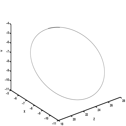
(b)

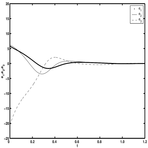
Figure 1: Synchronization of unstable limit cycle of Lorenz system. Here $(\sigma,\,b,\,r)=(10,\,8/3,\,24.5)$, $u=-5$, the time step-length is 0.001. (a) The unstable Limit cycle $\mathcal{C}$. (b) The evolution of synchronization error. Here $e_{1}=x_{s}-x_{m},\,e_{2}=y_{s}-y_{m},\,e_{3}=z_{s}-z_{m}.$

(a)
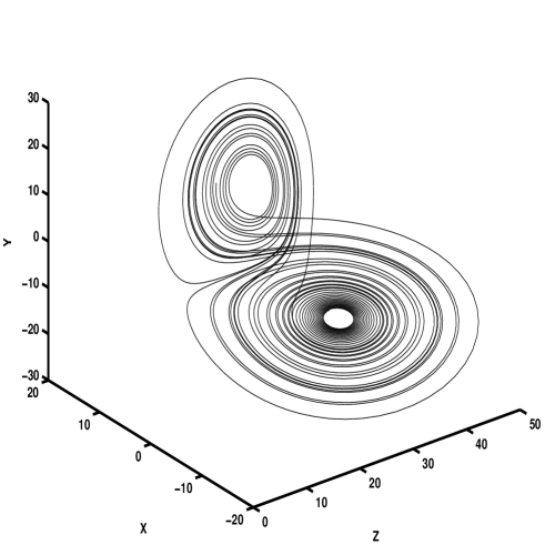
(b)

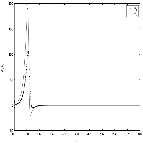
Figure 2: Chaos synchronization of Lorenz System. Here $(\sigma,\,b,\,r)=(10,\,8/3,\,28)$, $u=-6$, the time step-length is 0.008. (a) The chaotic attractor. (b) The evolution of synchronization error. Here, $e_{1}=x_{s}-x_{m},\,e_{2}=y_{s}-y_{m}.$

(a)
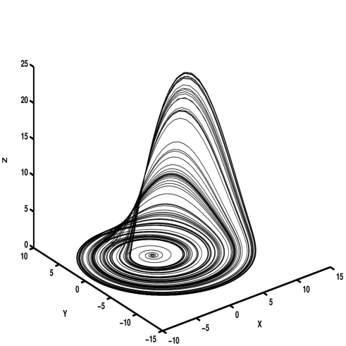
(b)

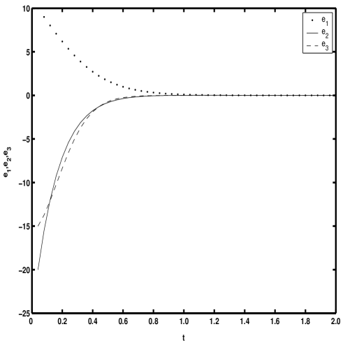
Figure 3: Chaos synchronization of Rössler System. Here $a=b=0.2$, $c=5.7$, $u=-6$, the time step-length is 0.04. (a) The chaotic attractor. (b) The evolution of synchronization error. Here, $e_{1}=x_{s}-x_{m},\,e_{2}=y_{s}-y_{m},\,e_{3}=z_{s}-z_{m}.$

[1] I.I. Blekman, Synchronization in science and technology, ASME Press, New York, 1988.

[2] L. M. Pecora, T. L. Carroll, Phys. Rev. Lett. 64, 821 (1990).

[3] A. Maybhate, and R.E. Amritkar, Phys. Rev. E 59, 284 (1999).

[4] J.W. Shuai, K.W. Wong and L.M. Cheng, Phys. Rev. E 56, 2272 (1997).

[5] C. Zhou and C.H. Lai, Phys. D 135, 1 (2000).

[6] S. Boccaletti, J. Kurths, G. Osipov, D. L. Valladares, C. S. Zhou, Phys. Rep. 366, 1 (2002).

[7] J. P. Yan and C. P. Li, Chaos, Solitons and Fractals 23, 1683 (2005).

[8] A. Ambrosetti and G. Prodi, A prime of nonlinear analysis, Cambridge University Press, Cambridge, 1993.

[9] C. P. Li and G. Chen, Chaos, Solitons and Fractals 18, 69 (2003).

[10] C. Sparrow, The Lorenz equations, bifurcation, chaos, and strange attractors, Springer-Verlag, New York, 1982.

[11] O. E. Rössler, Ann. N.Y. Acad. Sci. 316, 376 (1978).