Impact of noise on domain growth in electroconvection

Abstract

The growth and ordering of striped domains has recently received renewed attention due in part to experimental studies in diblock copolymers and electroconvection. One surprising result has been the relative slow dynamics associated with the growth of striped domains. One potential source of the slow dynamics is the pinning of defects in the periodic potential of the stripes. Of interest is whether or not external noise will have a significant impact on the domain ordering, perhaps by reducing the pinning and increasing the rate of ordering. In contrast, we present experiments using electroconvection in which we show that a particular type of external noise decreases the rate of domain ordering.

The study of domain ordering after a sudden change to a system (or a quench) has implications for a wide range of applications and fields, from processing binary mixtures of fluids to the organization of crystalline domains in a solid Bray (1994). Domain ordering occurs when different spatial regions of a system are in different states, and the size of these regions change with time. A common method to generate such a situation is to take a uniform system and subject it to a sudden change in external parameters such that the system can now exist in two or more degenerate states. Regions form that select from the possible states, creating an inhomogeneous system that proceeds to order. Our understanding of the ordering process focuses on the case when the system is spatially uniform within each domain. In this case, one can generally understand the coarsening, or domain ordering, by considering the motion of the topological defects in the system Bray (1994). The situation is less clear when the domains themselves contain spatial structure. In this regard, domains of stripes have received significant attention Elder et al. (1992); Cross and Meiron (1995); Christensen and Bray (1998); Harrison et al. (2000); Boyer and Vinals (2001); Harrison et al. (2002); Qian and Mazenko (2003, 2004); Purvis and Dennin (2001); Taneike and Shiwa (1997); Taneike et al. (2002); Boyer (2004).

Stripes, or more generally patterns, occur in a wide range of systems Cross and Hohenberg (1993); Gollub and Langer (1999), including convecting fluids, animal coats, polymer melts, and ferromagnets. Stripes occur both as an equilibrium state of the system, such as in diblock copolymers, and as a result of external driving, as in convection in fluids. Theoretical studies of the ordering of striped domains Elder et al. (1992); Cross and Meiron (1995); Christensen and Bray (1998); Boyer and Vinals (2001); Qian and Mazenko (2003, 2004); Taneike and Shiwa (1997); Taneike et al. (2002); Boyer (2004) have focused on studies of model equations, such as the Swift-Hohenberg equation. In general, simulations find that the growth of striped domains occurs slower than might be expected from our knowledge of the growth of uniform systems. This is typically characterized by the growth exponent. For sufficiently late times, it is postulated that the length scale of domains in these systems scales as a power of time, usually referred to as the growth exponent. For uniform domains in systems approaching an equilibrium state, it is known that the exponents are $1/2$ if the order parameter is not conserved and $1/3$ for a conserved order parameter Bray (1994). For striped systems, growth exponents of various values are reported, including $1/3$, $1/4$, and $1/5$. There is evidence that for sufficiently large quenches, the system becomes glassy, and scaling breaks down Boyer and Vinals (2001); Boyer (2004). Of particular interest to the work in this paper are simulations that focus on anisotropic systems Boyer (2004) and recent simulations that focus on the impact of noise on the coarsening of stripes Taneike and Shiwa (1997); Taneike et al. (2002). This will be discussed in more detail later.

The ordering of stripe domains has been studied experimentally both for the diblock copolymer case Harrison et al. (2000, 2002) and the electroconvection in a nematic liquid crystal Purvis and Dennin (2001); Kamaga et al. (2004a, b). The work with diblock colpolymers strongly suggests that topological defects play a central role in the ordering of stripe domains Harrison et al. (2002). The work in electroconvection is interesting because the system is an example of coarsening in an anisotropic, driven system. The work in this paper focuses on domain coarsening in this system.

Nematic liquid crystals are fluids in which the molecules exhibit long-range orientational order de Gennes and Prost (1993). The average axis along which the molecules are aligned is referred to as the director. By proper treatment of the boundaries, samples with uniform director alignment can be prepared. When an electric voltage is applied to such a sample, there is a critical voltage at which convective flow of the fluid occurs. There is a corresponding periodic variation of the director field. This pattern is known as electroconvection Bodenschatz et al. (1988); Kramer and Pesch (1995); Rehberg et al. (1989). When the axis of the convection rolls forms a nonzero angle with the undistorted director field, the pattern is referred to as oblique rolls. This is a degenerate state because patterns with an angle $\theta$ (zig rolls) and $-\theta$ (zag rolls) are degenerate. By applying a sudden increase in voltage from below to above the critical value, a pattern of zig and zag domains is created. This pattern coarsens, or orders, in time. The ordering of the system is consistent with power law growth in time Purvis and Dennin (2001), but the growth is anisotropic, occurring at different rates parallel and perpendicular to the director Kamaga et al. (2004a).

Because electroconvection is driven electrically, it is a relatively easy system for studies of the impact of noise. Simulations of an anisotropic Swift-Hohenberg model Boyer (2004) suggest that the pinning of defects is relevant to the coarsening of the domains in electroconvection. Simulations for isotropic systems suggest that noise can alter the dynamics of the domain growth by changing the potential in which the defects move, effectively acting as a thermal bath Taneike and Shiwa (1997); Taneike et al. (2002). Though these simulations were performed for isotropic systems, there is no obvious reason that a similar phenomenon would not occur in electroconvection.

In considering the impact of noise on the domain growth, one can imagine different types of noise. The two classic cases are additive noise and multiplicative noise. These are best defined in the context of an amplitude equation formulation (or envelope equation) in which the fast variation (the period corresponding to the fundamental pattern) is removed and only long wavelength changes in the pattern are studied. In this formalism, additive noise is described by the addition of a noise term to the equation that is not directly coupled with the amplitude Elder et al. (1992); Taneike and Shiwa (1997). Multiplicative noise is the addition of a term that consists of a noise factor multiplying the amplitude Taneike et al. (2002). Since it is standard to have the driving represented by an appropriate dimensionless parameter times the amplitude, multiplicative noise enters the equations as an additive factor to the driving term. A surprising feature of the theoretical studies is the finding that the rate of domain growth increases when the noise is sufficiently small Elder et al. (1992); Taneike and Shiwa (1997); Taneike et al. (2002). Since these two very different noise sources have the same impact, it is possible that any generic noise would increase the rate of coarsening.

The details of the experimental apparatus are described in Ref. Dennin (2000). The nematic liquid crystal N4 was doped with 0.1 wt% of tetra n-butylammonium bromide [${\rm(C_{4}H_{9})4NBr}$]. Commercial cells EHC with a quoted thickness of 25 $\mu$m and 1 cm² electrodes were used, giving an aspect ratio of 400. The cells were treated so that the director has a uniform planar alignment (parallel to the top and bottom of the plates). The direction of the undistorted director is taken as the x-axis and the direction perpendicular to the plates is taken as the z-axis. The y-axis is chosen to form a standard right-handed coordinate system. The average wavelength of the rolls was $51\ {\rm\mu m}$. The sample temperature was maintained at $35.0\pm 0.002\ {\rm{}^{\circ}C}$.

Figure 1: (a) A single cycle of a typical waveform that is used to drive electroconvection. A noise amplitude of 0.6 V is used so that it is visible to the reader. (b) Power spectrum for the signal plotted in (a).

Typically, an AC voltage of the form $V(t)=V_{o}\cos(\omega t)$ is applied perpendicular to the cell, where $V_{o}$ is the amplitude of the applied voltage and $\omega/2\pi$ is the driving frequency. For all of the experiments reported here, $V(t)=[V_{o}+\xi(t)]\cos(\omega t)$, where $\xi(t)$ is a random noise term chosen with a uniform probability from the range $-\xi_{m}\leq\xi(t)\leq\xi_{m}$. Figure 1 shows sample waveforms with their corresponding power spectra with $\xi_{m}=0.6\ {\rm V}$. The basically flat power spectra indicate the randomness of the noise. This was achieved by using a built-in pseudo-random number generator with a seed value that changes often, i.e. the time function which is the number of seconds elapsed since New Year 1970. After one cycle of the waveform is randomized, that cycle is the repeated to create a periodic random waveform.

It should be noted that the noise we add is similar to the multiplicative noise studied theoretically. However, two facts need to be considered when comparing our results to theory. First, we add the noise to the raw voltage and the control parameter is the square of the voltage. Second, because of experimental limitations, the noise has a periodic element as only a single cycle is generated randomly. Therefore, these experiments are focused on testing the generality of the result that noise increases the rate of growth of domains, and not on testing a specific class of noise, such as additive or multiplicative.

Figure 2: Plot of the critical voltage for the onset of electroconvection as a function of the noise amplitude. Notice, the transition at a noise amplitude of approximately 1.5 V.

The dimensional parameter $\epsilon=(V/V_{c})^{2}-1$ characterizes the depth of the quench. Here $V_{c}\approx 5.4\ {\rm V}$ is the onset voltage for electroconvection at the applied frequency ($f=\omega/2\pi$) of interest. For all of the experiments reported here, $f=500\ {\rm Hz}$. The introduction of noise did have a small effect on the onset voltage, as shown in Fig. 2. In order to study domain coarsening, voltage quenches were used that started from a uniform state and suddenly applied sufficient voltage to reach $\epsilon=0.2$, where $\epsilon$ is computed using $V_{c}$ in the absence of noise. This represents one particular type of quench to compare. The other option would be to have each quench be to the same value of $\epsilon$ relative to $V_{c}$ in the presence of the noise. However, the difference between these two choices is less than a few percent. At that level, we found the quench depth did not impact the domain ordering. We also define a relative noise strength $\eta=\xi_{m}/V_{c}$, where $V_{c}$ is again taken as the critical voltage in the absence of noise.

After the application of the quench, domains of zig and zag, separated by grain boundaries and vertical walls of dislocations, formed in approximately 30 seconds. As these domains evolved, images were taken every 30 seconds for 35 minutes. At 35 minutes, the system essentially is always a single domain within the field of view. For each noise amplitude, the results of twenty quenches were averaged. Noise amplitudes ranging from $\eta=0$ to $\eta=0.2$ were used.

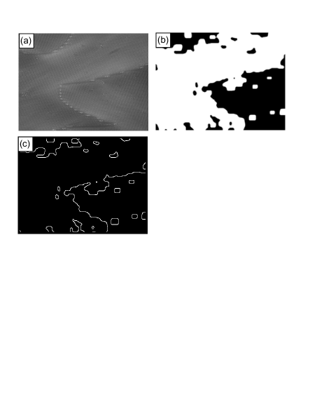
Figure 3: Three images illustrating the process by which domains are defined. The images are all $2.03\ {\rm mm}\times 1.41\ {\rm mm}$(a) Raw image of electroconvection showing two regions of zag rolls in between two regions of zig rolls. (b) The processed image in which zag is white and zig is black. (c) The extracted domain walls from image (b).

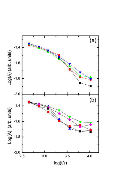
Figure 4: (color online)Both plots give the normalized boundary area as a function of time normalized by the director relaxation time. (a) is for noise strengths $\eta=0$ ($\blacksquare$), 0.019 (red $\bullet$), 0.037 (green $\blacktriangle$), 0.056 (blue $\blacktriangledown$) and (b) is for noise strengths 0.074 ($\blacksquare$), 0.093(red $\bullet$), 0.148 (blue $\blacktriangle$), 0.167 (green $\blacktriangledown$), and 0.185 (magenta $\blacklozenge$). There is a qualitative difference in the temporal evolution in the two regimes, suggesting a transition in the temporal evolution as a function of the noise strength.

In order to measure the degree of domain coarsening that has taken place, we look at the length of the boundaries between domains. To do this, a program was developed using IDL 6.1. This program takes advantage of the fact that the product $k_{x}k_{y}$ for the wavevector of the zig pattern is positive while for zag it is negative. The optical image is translated into a representation of the sign of $k_{x}k_{y}$, with regions of black and white corresponding to plus and minus, or zig and zag. The program then uses thresholding techniques to isolate the boundaries between domains that are mixtures of black and white pixels. The number of boundary pixels represents a way to measure how far the domain coarsening has progressed. This method is based on the algorithm described in Ref. Egolf et al. (1998), and the details as applied to our system are given in Ref. Purvis and Dennin (2001). Figure 3 shows the typical results of the program for an image that is taken 6 minutes after the quench.

The main results of the paper are illustrated in Fig. 4. Here the time evolution of the average domain wall length is plotted for a number of different noise strengths. Time is measured from immediately after the quench. Also, time is scaled by the director relaxation time, $\tau\equiv\gamma_{1}d^{2}/(\pi^{2}K_{11})=0.2\ {\rm s}$. Here $\gamma_{1}$ is a rotational viscosity; $K_{11}$ is the splay elastic constant; and $d$ is the thickness of the cell. There are two main results.

Figure 4 illustrates that the evolution is slowed by increasing the noise strength. At a noise strength of 0.07, there is a qualitative change in the evolution of the system. Below 0.07, the system appears to be continuing to evolve on the time scale for which observation was possible. Above 0.07, the system plateaus at the the later times and the evolution is “frozen”. Another way to view this is that the late time measure of domain wall length is significantly larger for quenches with a noise strength above 0.07, implying that the coarsening dynamics have slowed down. This is opposite previous theoretical results Elder et al. (1992); Taneike and Shiwa (1997); Taneike et al. (2002). The most likely explanation is the fact that we are using noise that is not purely multiplicative or additive, but the details of why this type of noise slows the dynamics requires further study.

Another interesting result of applying this type of noise to the system is the global impact on the pattern. Under sufficiently strong amplitude, one would expect the noise to cause the spontaneous generation of dislocation pairs, resulting in some level of chaotic dynamics. We observed no evidence for such a transition, even at noise strengths as high as 0.9. This behavior has interesting implications for the nature of coupling between the applied noise and the pattern dynamics. The noise clearly impacted the dynamics of the system by significantly slowing domain growth at a critical value. However, the lack of any generation of defects is probably connected to the fact that the noise is applied directly to the voltage and that the driving force is given by the root mean square value of the voltage. The impact of this should be explored further with simulations and by experimental studies of different noise sources. It also presents an interesting pattern situation in which the dynamics of a system can be controlled to some degree by noise without having a substantial impact on the qualitative aspects of the pattern.