Synchronization of Coupled Chaotic Dynamics on Networks

Abstract

We review some recent work on the synchronization of coupled dynamical systems on a variety of networks. When nodes show synchronized behaviour, two interesting phenomena can be observed. First, there are some nodes of the floating type that show intermittent behaviour between getting attached to some clusters and evolving independently. Secondly, two different ways of cluster formation can be identified, namely self-organized clusters which have mostly intra-cluster couplings and driven clusters which have mostly inter-cluster couplings.

I Introduction

The phenomena of synchronization of several dynamical variables or oscillators is important for many physical and biological systems [1]. Some important physical systems showing synchronization are arrays of lasers [2], microwave oscillators and superconducting Josephson junctions [1] while some important biological systems are synchronous firing of neurons [3], networks of pacemaker cells in the heart [4], metabolic synchrony in yeast cell suspensions [5], congregations of synchronously flashing fireflies [6], and cricket that chirp in unison [7].

Coupled oscillators were first studied by Winfree [8] and Kuramoto [9]. The Kuramoto model describes a large population of coupled limit cycle oscillators with random frequencies. If the coupling strength exceeds a critical threshold, the system exhibits a phase transition to a synchronous state where several oscillators synchronize and lock to a common frequency [10].

Two important developments have regenerated interest in the study of synchronization of dynamical variables. First is the recognition that chaotic dynamical systems can show exact or phase synchronization [11]. Second is the observation that several natural systems have an underlying geometric structure which can be described by complex networks [12, 13]. This has opened up the possibility of discovering new interesting phenomena in coupled dynamical systems on complex networks. We discuss some of these aspects in this article.

Several networks in the real world consist of dynamical elements interacting with each other and the interactions define the links of the network. Several of these networks have a large number of degrees of freedom and it is important to understand their dynamical behaviour. A general model of coupled dynamical systems on networks will consist of the following three elements.

1. The evolution of uncoupled elements.

2. The nature of couplings.

3. The topology of the network.

Most of the earlier studies of synchronized cluster formation in coupled chaotic systems have focused on networks with large number of connections ($\sim N^{2}$) [14] or nearest neighbour couplings on lattice models. Recently, we have considered complex networks with number of connections of the order of $N$ [15]. This small number of connections allows us to study the role that different connections play in synchronizing different nodes and the mechanism of synchronized cluster formation. The study reveals two interesting phenomena. First, when nodes form synchronized clusters, there can be some nodes which show an intermittent behaviour between independent evolution and evolution synchronized with some cluster. Secondly, the cluster formation can be in two different ways, driven and self-organized phase synchronization [15]. The connections or couplings in the self-organized phase synchronized clusters are mostly of the intra-cluster type while those in the driven phase synchronized clusters are mostly of the inter-cluster type. We will briefly review these features in this article.

II Synchronization of dynamical systems

Synchronization of different dynamical variables can be defined in several ways. Exact synchronization corresponds to the situation where the dynamical variables have identical values, i.e. two dynamical variables $x_{i}$ and $x_{j}$ are exactly synchronized if $x_{i}(t)=x_{j}(t)$ [16]. Generalised synchronization is defined by some functional relation between the dynamical variables [17]. Several other types of synchronization such as phase synchronization [18], lag synchronization [19], anticipatory synchronization [20] etc. have been defined.

A Kuramoto model of coupled oscillators

Kuramoto model of coupled oscillators can be introduced through the evolution equation [9]

$$\dot{\theta}_{i}=\omega_{i}+\frac{K}{N}\sum_{j=1}^{N}\sin(\theta_{j}-\theta_{i}),\,\,i=1,\ldots,N,$$ (1)

where $\theta_{i}$ is the phase of oscillator $i$, $\omega_{i}$ is its natural frequency and $K$ is the coupling strength. Phase synchronization of the oscillators can be studied using the complex order parameter defined as

$\displaystyle re^{i\psi}=\frac{1}{N}\sum_{j=1}^{N}e^{i\theta_{j}}$

where $r$ measures the phase coherence, and $\psi$ is the average phase. Clearly, $r$ vanishes for a uniform distribution of phases $\theta_{i}$, and $r=1$ if all $\theta_{i}$ are equal. The evolution equation for the phases can be written as,

$\displaystyle\dot{\theta}_{i}=\omega_{i}+Krsin(\psi-\theta_{i})$

This is a mean field form of the equation. For $K$ less than some threshold $K_{c}$, the oscillators show unsynchronized behaviour. But, when $K>K_{c}$, the oscillator population splits into two groups, the oscillators near the center of the frequency distribution lock together at some frequency $\omega_{0}$ to form a synchronized cluster, while those in the tail retain their natural frequencies and drift relative to the synchronized cluster. This state is often called partially synchronized state. With further increase in $K$, more and more oscillators are recruited into the synchronized clusters [9, 21, 22].

Kuramoto’s model was originally motivated by biological oscillators [8], but it has found applications in many diverse systems such as flavour evolution of neutrinos [23], arrays of Josephson junction [24], semiconductor lasers [25] and in several other systems [26, 27].

B Synchronization of chaotic systems

Pecora and Carroll showed that two identical chaotic systems can synchronize if approrpiate driving mechanisms are introduced [11]. Let ${\bf x}$ be an $n$ dimensional dynamical variable evolving as (drive system)

$$\dot{\bf x}={\bf f}({\bf x}).$$ (2)

Divide the dynamical variables into two parts, ${\bf x}=({\bf x}_{d},{\bf x}_{r})$, a drive part and a response part. Consider another dynamical system (response system) given by

$$\dot{\bf x}^{{}^{\prime}}={\bf f}({\bf x}_{d},{\bf x}_{r}^{{}^{\prime}}).$$ (3)

where the drive variables ${\bf x_{d}}$ are obtained from Eq. (2). Under suitable conditions, i.e. the conditional Lyapunov exponents are negative, the response variable ${\bf x}_{r}^{{}^{\prime}}$ synchronize with those of the drive system, ${\bf x}_{r}$. The conditional Lyapunov exponents are obtained by considering the subspace of response variables. The important interesting feature is that the variables synchronize even when they are evolving chaotically. Thus we do not have frequency locking, but we can have phase synchronization if a suitable phase variable can be defined [18]. Such phase synchronization is observed in several biological systems [1]

C Coupled dynamics on Complex Networks

Several complex systems have underlying structures that are described by networks or graphs [12, 13]. Recent interest in networks is due to the discovery that several naturally occurring networks come under some universal classes and they can be simulated with simple mathematical models, viz small-world networks [28], scale-free networks [29] etc.

Consider a network of $N$ nodes and $N_{c}$ connections (or couplings) between the nodes. Let each node of the network be assigned an $m$-dimensional dynamical variable ${\bf x}^{i},i=1,2,\ldots,N$. A very general dynamical evolution can be written as

$$\frac{d{\bf x}_{i}}{dt}={\bf F}(\{{\bf x}_{i}\}).$$ (4)

Here, we consider a separable case and the evolution equation can be written as,

$$\frac{d{\bf x}_{i}}{dt}={\bf f}({\bf x}_{i})+\frac{\epsilon}{k_{i}}\sum_{j\in\{k_{i}\}}{\bf g}({\bf x}_{j}).$$ (5)

where $\epsilon$ is the coupling constant, $k_{i}$ is the degree of node $i$, and $\{k_{i}\}$ is the set of nodes connected to the node $i$. A sort of diffusion version of the evolution equation (5) is

$$\frac{d{\bf x}_{i}}{dt}={\bf f}({\bf x}_{i})+\frac{\epsilon}{k_{i}}\sum_{j\in\{k_{i}\}}\left({\bf g}({\bf x}_{j})-{\bf g}({\bf x}_{i})\right).$$ (6)

Discrete versions of Eqs. (5) and (6) are

$${\bf x}_{i}(t+1)={\bf f}({\bf x}_{i}(t))+\frac{\epsilon}{k_{i}}\sum_{j\in\{k_{i}\}}{\bf g}({\bf x}_{j}(t)).$$ (7)

and

$${\bf x}_{i}(t+1)={\bf f}({\bf x}_{i}(t))+\frac{\epsilon}{k_{i}}\sum_{j\in\{k_{i}\}}\left({\bf g}({\bf x}_{j}(t))-{\bf g}({\bf x}_{i}(t))\right).$$ (8)

In numerical studies, for the discrete evolution we can use any descrete map such as logistic or circle maps while for the continuous case we can use chaotic systems such as Lorenz or Rössler systems.

As noted before synchronization of coupled dynamical systems [1] is manifested by the appearance of some relation between the functionals of different dynamical variables. When the number of connections in the network is small ($N_{C}\sim N$) and when the local dynamics of the nodes (i.e. function $f(x)$) is in the chaotic zone, and we look at exact synchronization, only few synchronized clusters with small number of nodes are formed. However, when we look at phase synchronization, synchronized clusters with larger number of nodes are obtained.

III General properties of synchronized dynamics on complex networks

We consider some general properties of synchronized dynamics. They are valid for any coupled discrete and continuous dynamical systems. Also, these properties are applicable for exact as well as phase or any other type of synchronization and are independent of the type of network.

A Behavior of individual nodes

As the network evolves, it splits into several synchronized clusters. Depending on their asymptotic dynamical behaviour the nodes of the network can be divided into three types.
(a) Cluster nodes: A node of this type synchronizes with other nodes and forms a synchronized cluster. Once this node enters a synchronized cluster it remains in that cluster afterwards.
(b) Isolated nodes: A node of this type does not synchronize with any other node and remains isolated for all the time.
(c) Floating Nodes: A node of this type keeps on switching intermittently between an independent evolution and a synchronized evolution attached to some cluster.

Of particular interest are the floating nodes and we will discuss some of their properties afterwards.

B Mechanism of cluster formation

The study of the relation between the synchronized clusters and the couplings between the nodes represented by the adjacency matrix $C$ shows two different mechanisms of cluster formation [15, 30].
(i) Self-organized clusters: The nodes of a cluster can be synchronized because of intra-cluster couplings. We refer to this as the self-organized synchronization and the corresponding synchronized clusters as self-organized clusters.
(ii) Driven clusters: The nodes of a cluster can be synchronized because of inter-cluster couplings. Here the nodes of one cluster are driven by those of the others. We refer to this as the driven synchronization and the corresponding clusters as driven clusters.

In numerical studies it is possible to observe ideal clusters of both the types, as well as clusters of the mixed type where both ways of synchronization contribute to cluster formation. Fig. 1 shows some examples of ideal as well as mixed clusters in coupled map networks [15]. In general we find that the scale free networks and the Caley tree networks lead to better cluster formation than the other types of networks with the same average connectivity.

FIG. 1.: The figure shows node versus node diagrams for several examples illustrating the self-organized and driven phase synchronization and the variety of clusters that are formed. The examples are for coupled maps on a scale free network with $N=50$, the local dynamics is given by the logistic $4x(1-x)$ and the coupling function is linear. The solid circles show that the two corresponding nodes are coupled (i.e. $C_{ij}=1$) and the open circles show that the corresponding nodes are phase synchronized. In each case the node numbers are reorganized so that nodes belonging to the same cluster are numbered consecutively and the clusters get displayed in decreasing sizes. (a) Figure shows turbulent phase for coupling constant $\epsilon=0.10$. (b) An ideal self-organized phase synchronization for $\epsilon=0.16$. (c) Mixed behavior for $\epsilon=0.32$. (d) An ideal driven phase synchronization for $\epsilon=0.90$.

Geometrically the two mechanisms of cluster formation can be easily understood by considering a tree type network. A tree can be broken into different clusters in different ways.
(a) A tree can be broken into two or more disjoint clusters with only intra-cluster couplings by breaking one or more connections. Clearly, this splitting is not unique and will lead to self-organized clusters. Figure 2(a) shows a tree forming two synchronized clusters of self-organized type. This situation is similar to an Ising ferromagnet where domains of up and down spins can be formed.
(b) A tree can also be divided into two clusters by putting connected nodes into different clusters. This division is unique and leads to two clusters with only inter-cluster couplings, i.e. driven clusters. Figure 2(b) shows a tree forming two synchronized clusters of the driven type. This situation is similar to an Ising anti-ferromagnet where two sub-lattices of up and down spins are formed.
(c) Several other ways of splitting a tree are possible. E.g. it is easy to see that a tree can be broken into three clusters of the driven type. This is shown in figure 2(c). There is no simple magnetic analog for this type of cluster formation. It can be observed close to a period three orbit. We note that four or more clusters of the driven type are also possible. As compared to the cases (a) and (b) discussed above which are commonly observed, the clusters of case (c) are not so common and are observed only for some values of the parameters.

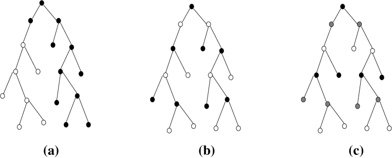
FIG. 2.: Different ways of cluster formation in a tree structure are demonstrated. The open, solid and gray circles show nodes belonging to different clusters. (a) shows two clusters of the self-organized type, (b) shows two clusters of driven type and (c) shows three clusters of the driven type.

IV Linear stability analysis

A suitable network to study the stability of self-organized synchronized clusters is the globally coupled network. The stability of globally coupled maps is well studied in the literature [31, 32, 33]. An ideal example to consider the stability of the driven synchronized state is a complete bipartite network. A complete bipartite network consists of two sets of nodes with each node of one set connected with all the nodes of the other set and no connection between the nodes of the same set. Let $N_{1}$ and $N_{2}$ be the number of nodes belonging to the two sets. We define a bipartite synchronized state as the one that has all $N_{1}$ elements of the first set synchronized to some value, say ${\bf X}_{1}(t)$, and all $N_{2}$ elements of the second set synchronized to some other value, say ${\bf X}_{2}(t)$.

All the eigenvectors and the eigenvalues of the Jacobian matrix for the bipartite synchronized state can be determined explicitly. The eigenvectors of the type $(\alpha,\ldots,\alpha,\beta,\ldots,\beta)^{T}$ determine the synchronization manifold and this manifold has dimension two. All other eigenvectors correspond to the transverse manifold. Lyapunov exponents corresponding to the transverse eigenvectors for Eq. (8) with one dimensional variables and $g(x)=f(x)$ are

$$\lambda_{1} = \ln|(1-\epsilon)|+\frac{1}{\tau}\lim_{\tau\to\infty}\sum^{\tau}_{t=1}\ln|f^{\prime}(X_{1})|,$$ (9)

$$\lambda_{2} = \ln|(1-\epsilon)|+\frac{1}{\tau}\lim_{\tau\to\infty}\sum^{\tau}_{t=1}\ln|f^{\prime}(X_{2})|,$$ (10)

and $\lambda_{1}$ and $\lambda_{2}$ are respectively $N_{1}-1$ and $N_{2}-1$ fold degenerate [30]. Here, $f^{\prime}_{(}X_{1})$ and $f^{\prime}_{(}X_{2})$ are the derivatives of $f(x)$ at $X_{1}$ and $X_{2}$ respectively. The synchronized state is stable provided the transverse Lyapunov exponents are negative. If $f^{\prime}$ is bounded then from Eqs. (10) we see that for $\epsilon$ larger than some critical value, $\epsilon_{b}(<1)$, bipartite synchronized state will be stable. Note that this bipartite synchronized state will be stable even if one or both the remaining Lyapunov exponents corresponding to the synchronization manifold are positive, i.e. the trajectories are chaotic. The linear stability analysis for other type of couplings and dynamical systems can be done along similar lines.

V Floating nodes

We had noted earlier that the nodes can be divided into three types, namely cluster nodes, isolated nodes and floating nodes, depending on the asymptotic behavior of the nodes. Here, we discuss some properties of the floating nodes which show an intermittent behavior between synchronized evolution with some cluster and an independent evolution.

Let $\tau$ denote the residence time of a floating node in a cluster (i.e. the continuous time interval that the node is in a cluster). Figure 3 plots the frequency of residence time $\nu(\tau)$ of a floating node as a function of the residence time $\tau$. A good straight line fit on log-linear plot shows an exponential dependence,

$$\nu(\tau)\sim\exp(-\tau/\tau_{r})$$ (11)

where $\tau_{r}$ is the typical residence time for a given node. We have also studied the distribution of the time intervals for which a floating node is not synchronized with a given cluster. This also shows an exponential distribution.

FIG. 3.: The figure plots the frequency of residence time $\nu(\tau)$ of a floating node in a cluster as a function of the residence time $\tau$. A good straight line fit on log-linear plot shows exponential dependence.

Several natural systems show examples of floating nodes, e.g. some birds may show intermittent behaviour between free flying and flying in a flock. An interesting example in physics is that of particles or molecules in a liquid in equilibrium with its vapor where the particles intermittently belong to the liquid and vapor. Under suitable conditions it is possible to argue that the residence time of a tagged particle in the liquid phase should have an exponential distribution [30], i.e. a behavior similar to that of the floating nodes (Eq. (11)).

VI Conclusion and Discussion

We have briefly discussed synchronization properties of coupled dynamical elements on complex networks. In the course of time evolution these dynamical elements form synchronized clusters.

In several cases when synchronized clusters are formed there are some isolated nodes which do not belong to any cluster. More interestingly there are some floating nodes which show an intermittent behavior between an independent evolution and an evolution synchronized with some cluster. The residence time spent by a floating node in the synchronized cluster shows an exponential distribution.

We have identified two mechanisms of cluster formation, self-organized and driven phase synchronization. For self-organized clusters intra-cluster couplings dominate while for driven clusters inter-cluster couplings dominate.

REFERENCES

- [1] A. Pikovsky, M. Rosenblum and J. Kurth, Synchronization : A universal concept in nonlinear dynamics (Cambridge University Press, 2001).
- [2] Z. Jiang, M. McCall, J. Opt. Soc. Am. 10, 155 (1993).
- [3] P. A. Robinson, J. J. Wright and C. J. Rennie, Phys. Rev. Lett. 57, 4578, (1998).
- [4] C. S. Peskin, Mathematical Aspects of Heart Physiology (Courant Institute of Mathematical Science Publication, New York, 1975, pp. 268).
- [5] J. Aldridge, E. K. Pye, Nature 259, 670 (1976).
- [6] J. Buck, E. Buck, Scientific Am. 234, 74 (1996).
- [7] T. J. Walker, Science 166, 891 (1969).
- [8] A. T. Winfree, The Geometry of Biological Time (Springer-Verlag, New York, 1980).
- [9] Y. Kuramoto, Chemical Oscillations, Waves, and Turbulence (Springer- Verlag, Berlin, 1984).
- [10] A. T. Winfree, J. Theoret. Biol. 16 15 (1967).
- [11] L. M. Pecora and T. L. Carroll, Phys. Rev. Lett. 64, 821 (1990).
- [12] S. H. Strogatz, Nature 410, 268 (2001) and references therein.
- [13] R. Albert and A. L. Barabäsi, Rev. Mod. Phys. 74, 47 (2002) and references therein.
- [14] K. Kaneko, Physica D124 (1998) 322.
- [15] S. Jalan, R. E. Amritkar, Phys. Rev. Lett. 90 (2003) 014101.
- [16] H. Fujisaka and T. Yamada, Prog. Theor. Phys. 69, 32 (1983).
- [17] H. F. Rulkov, M. M. Sushchik, L. S. Tsimring and H. D. I. Abarbanel, Phys. Rev. E 51, 980 (1995).
- [18] M. G. Rosenblum, A. S. Pikovsky, and J. Kurth, Phys. Rev. Lett. 76, 1804 (1996).
- [19] M. G. Rosenblum, A. S. Pikovsky, and J. Kurth, Phys. Rev. Lett. 78, 4193 (1997).
- [20] H. U. Voss, Phys. Rev. E 61, 5115 (2000).
- [21] J. D. Crawford, J. Statist. Phys., 74, 1047 (1994); J. D. Crawford and K. T. R. Davies, Physica D 125 1 (1999).
- [22] S. H. Strogatz, Physica D, 143 1 (2000).
- [23] J. Pantaleone, Phys. Rev. D 58, 3002 (1998).
- [24] K. Wiesenfeld, P. Colet, S. H. Strogatz, Phys. Rev. E 57, 1563 (1998).
- [25] G. Kozyreff, A. G. Vladimirov and P. Mandal, Phys. Rev. Lett. 85, 3809 (2000).
- [26] Y. Maistrenko, O. Popovych, O. Burylko and P. A. Tass, Phys. Rev. Lett. 93, 841021 (2004)
- [27] M. G. Earl and S. H. Strogatz, Phys. Rev. E 67, 036204 (2003).
- [28] D. J. Watts and S. H. Strogatz, ’Collective Dynamics of Small World Networks,’ Nature (London) 393, 440 (1998).
- [29] A. -L. Barabäsi, R. Albert, ‘Emergence of Scaling in Random Networks,’ Science 286, 509 (1999).
- [30] S. Jalan, R. E. Amritkar and C. K. Hu, unpublished.
- [31] H. Fujisaka and T. Yamada, Prog. Theo. Phys. 69, 32 (1983).
- [32] P. M. Gade, Phys. Rev. E54 (1996) 64.
- [33] M. Ding and W. Yang, Phys Rev E56 (1997) 4009.