Synchronization by Reactive Coupling and Nonlinear Frequency Pulling

Abstract

We present a detailed analysis of a model for the synchronization of nonlinear oscillators due to reactive coupling and nonlinear frequency pulling. We study the model for the mean field case of all-to-all coupling, deriving results for the initial onset of synchronization as the coupling or nonlinearity increase, and conditions for the existence of the completely synchronized state when all the oscillators evolve with the same frequency. Explicit results are derived for Lorentzian, triangular, and top-hat distributions of oscillator frequencies. Numerical simulations are used to construct complete phase diagrams for these distributions.

I Introduction

Increasingly the collective behavior displayed by groups of interacting dynamical components, each of which may be capable of a full range of complex dynamics, is essential to understanding and ultimately designing systems. Examples in biology, physics, and engineering are diverse, ranging from understanding sensory perception to the design of antennas capable of simultaneously sending and receiving signals at the same frequency. While in general the dynamical components may be functionally distinct and heterogeneous, in many examples one is interested in the collective behavior displayed by a group of similar coupled elements. One commonly studied example is the synchronization of oscillating subsystems that interact.

The ability of a group of coupled oscillators to synchronize despite a distribution in individual frequencies is a broadly applicable phenomenon. In physical systems coherent oscillations can be used to enhance detector sensitivity or increase the intensity of a power source. Synchronization is also important in biological systems where the collective behaviors in populations of animals, such as the synchronized flashing of fireflies or the coherent oscillations observed in the brain, serve as examples. Including a distribution in individual frequencies in an otherwise homogeneous ensemble captures some of the inevitable differences that group members will possess.

Although synchronization is often put forward as an example of the importance of understanding nonlinear phenomena, the intuition for it, and indeed the subsequent mathematical discussion, often reduces to simple linear ideas. For example, the famous example of Huygens’ clocks BSRW02 can be understood in terms of a linear coupling of the two pendulums through the common mounting support. Then the larger damping of the symmetric mode (coming from the larger, dissipative motion of the common support) compared with the antisymmetric mode leads at long times to a synchronized state of the two pendulums oscillating in antiphase. The nonlinearity in the system is simply present in the individual motion of each pendulum; specifically in the mechanism to sustain the oscillations. Without the drive, the oscillators would still become synchronized through the faster decay of the even mode, albeit in a slowly decaying state. Rather than this mode-dependent dissipation mechanism, one might expect synchronization to arise from the intrinsically nonlinear effect of the frequency pulling of one oscillator by another. Furthermore, the model describing the two pendulums, as well as most other models used to show synchronization, has dissipative coupling between the oscillators. In contrast, many physical situations have mainly reactive coupling.

Nanoscale mechanical oscillator arrays are one example that offer significant potential in a range of technologies BR02 ,SHSICC03 . Due to the scales and numbers in these arrays, active control of individual oscillators poses a number of challenging problems. Synchronization offers a potentially appealing alternative in some applications. One notable characteristic of these arrays is the predominantly reactive coupling due to elastic or electrostatic interactions. This context is the motivation for our work. In particular, we study the model

$$\dot{z}_{m}=i(\omega_{m}-\alpha|z_{m}|^{2})z_{m}+(1-\left|z_{m}\right|^{2})z_{m}+\frac{K+i\beta}{N}\sum_{n=1}^{N}(z_{n}-z_{m}),$$ (1)

where $z_{m}$ is a complex number representing the amplitude $r_{m}$ and phase $\theta_{m}$ of the mth oscillator $z_{m}=r_{m}e^{i\theta_{m}}$. The natural frequency $\omega_{m}$ of each oscillator is chosen from a distribution $g(\omega)$. We call the width of the distribution $w$. Coefficients of the terms for nonlinear frequency pulling ($\alpha$), dissipative coupling ($K$), and reactive coupling ($\beta$) serve as model parameters. The coupling is taken to be infinite range or all-to-all.

In this paper we study the roles of nonlinear frequency pulling and reactive coupling in the absence of the dissipative coupling using Eq. (1) with $\alpha\neq 0,\beta\neq 0,K=0$. In addition the distribution $g(\omega)$ of the $\omega_{m}$ must be specified. We study the case of positive $\alpha$ and $\beta$; for a symmetric distribution $g(\omega)$ the results are the same changing the sign of both $\alpha$ and $\beta$.

Alternatively, when only nonlinear saturation and dissipative coupling are present ($\alpha=\beta=0,K\neq 0$) Eq. (1) reduces to

$$\dot{z}_{m}=(i\omega_{m}+1-\left|z_{m}\right|^{2})z_{m}+\frac{K}{N}\sum_{n=1}^{N}(z_{n}-z_{m}).$$ (2)

The behavior for general $w$ and $K$ of Eq. (2) has been analyzed by Matthews et al. MMS91 . If the width $w$ of the distribution $g(\omega)$ is narrow, so that the time evolution of the magnitudes $\left|z_{m}\right|$ is fast compared with that of the phase dispersion, and $K$ is small, $\left|z_{m}\right|$ rapidly relaxes to a value close to unity, and the only remaining variable for each array member is the phase $\theta_{m}$. Equation (2) can then be reduced to a simple form W67 ,K75 , often known as the Kuramoto model

$$\dot{\theta}_{m}=\omega_{m}+\frac{K}{N}\sum_{n=1}^{N}\sin(\theta_{n}-\theta_{m}),$$ (3)

that has been the subject of numerous studies ABVRS05 . In the absence of coupling each oscillator in this model would simply advance at a rate that is constant in time, but with some dispersion of frequencies over the different elements. Equation (3) is an abstraction from the equations describing most real oscillator systems, leaving out many important physical features.

The complex notation of Eq. (1) suggests the introduction of a complex order parameter $\psi$ to measure the coherence of the oscillations

$$\psi=R\,e^{i\Theta}=\frac{1}{N}\sum_{n=1}^{N}r_{n}e^{i\theta_{n}},$$ (4)

with $r_{n}=1$ for the Kuramoto model, and then the equation of motion can be written [take the imaginary part of $\psi e^{-i\theta_{m}}$ in Eq. (4) to evaluate the sum appearing in Eq. (3)] as

$$\dot{\theta}_{m}=\omega_{m}+KR\sin(\Theta-\theta_{m}).$$ (5)

Thus the behavior of each oscillator is given by its tendency to lock to the phase of the order parameter. The term $KR\sin(\Theta-\theta_{m})$ acts as a locking force, and locking occurs for all oscillators with frequencies satisfying $\left|\omega_{m}\right|<KR$, with the locked oscillator phase given by $\Theta+\sin^{-1}(\omega_{m}/KR)$. The magnitude $R$ of the order parameter must then be determined self-consistently via Eq. (4). The generalization of the locking force to apply to the model Eq. (1) will be a conspicuous feature of our work.

Equation (3) is known to show rich behavior, including, in the large $N$ limit, a sharp synchronization transition at some value of the coupling constant $K=K_{c}$ K75 , which depends on the frequency distribution of the uncoupled oscillators $g(\omega)$. The transition is from an unsynchronized state with $\psi=0$ in which the oscillators run at their individual frequencies, to a synchronized state with $\psi\neq 0$ in which a finite fraction of the oscillators lock to a single frequency. The transition at $K_{c}$ has many of the features of a second order phase transition, with universal power laws and critical slowing down K75 , as well as a diverging response to an applied force S88 .

We present a detailed analysis of the model Eq. (1) with $K=0$ describing the synchronization of an oscillator ensemble involving reactive coupling between the elements, which then leads to synchronization through nonlinear frequency pulling. We begin in Sec. II by deriving Eq. (1) as a description of arrays of nanoelectromechanical oscillators. We then discuss the solutions to Eq. (1) for a variety of symmetric distributions in intrinsic frequencies $g(\omega)$. Common solution types exist for the three distinct types of frequency distributions we studied. In Sec. III we introduce these solutions and the measures we use to describe them. We begin the analysis in Sec. IV by moving to a continuum description to derive synchronization conditions. We are able to analyze the existence of two behavior types in closed form: the unsynchronized solution in Sec. V and the fully locked synchronized behavior in Sec. VI. Results from our analytical arguments are combined with those from simulations to present the solutions and associated phase diagram for each frequency distribution in Sec. VII. We begin these by considering an unbounded symmetric frequency distribution in the form of a Lorentzian in Sec. VII.1. Continuing in this section we then approximately double the distribution width to discuss some interesting characteristics of the well-ordered synchronized solutions as well as changes to the bifurcations. In contrast, Sec. VII.2 presents the results for a bounded distribution when all frequencies over some range are equally likely (a top-hat distribution). This is followed in Sec. VII.3 by the case of a symmetric unimodal frequency spread, namely a triangular distribution. Finally, conclusions are made in Sec. VIII.

A brief account of some results for the model Eq. (1) has been reported previously CZLR04 .

II Connection with Mechanical Oscillators

Although the main focus of this paper is analyzing the behavior of Eq. (1) we first show how such an equation might arise from the equations of motion of physical oscillators. As an example consider the system defined by

$$\ddot{x}_{n}+\omega_{n}^{2}x_{n}-\nu(1-x_{n}^{2})\dot{x}_{n}+ax_{n}^{3}-D[x_{n}-\tfrac{1}{2}(x_{n+1}+x_{n-1})]=0.$$ (6)

The first two terms describe uncoupled harmonic oscillators. We suppose the uncoupled oscillators have a linear frequency that is near unity by an appropriate scaling of the time variable

$$\omega_{n}^{2}=1+\delta_{n},\quad\delta_{n}\ll 1.$$ (7)

The third term is a negative linear damping, which represents an energy source to sustain the oscillations, and positive nonlinear damping, so that the oscillation amplitude saturates at a finite value. Again this saturation value is chosen to be of order unity by an appropriate scaling of the displacements $x_{n}$. For an example of an effective negative linear damping term in a micromechanical oscillator see references ZZOTSICPC01 ; IKARC05 . One could also imagine implementing such an effect with an electronic feedback loop sensing each oscillator velocity and driving the oscillator with an appropriate phase. The first three terms of Eq. (6) comprise a set of uncoupled van der Pohl oscillators. The term $ax_{n}^{3}$ describes a stiffening of the spring constant (for $a>0$) and is a reactive nonlinear term that leads to an amplitude dependent shift of the resonant frequency. With $\nu=0$ this would give us Duffing oscillators. The final term is a nearest neighbor coupling between the oscillators, depending on the difference of the displacements. This is a reactive term, that conserves the energy of the system. Others AEK90 have considered nonlinear oscillators coupled through their velocities; this is a dissipative coupling that would lead to $K\neq 0$ in the amplitude-phase reduction.

The complex amplitude equation (1) holds if the parameters $\nu,\alpha,D,\delta_{n}$ are sufficiently small. In this case the equations of motion are dominated by the terms describing simple harmonic oscillators at frequency one, and the time dependence remains close to $e^{\pm it}$. To formalize the smallness of $\nu,\alpha,D,\delta_{n}$ we introduce a small parameter $\varepsilon$ and write $\nu=\varepsilon\bar{\nu}$, $\delta_{n}=\varepsilon\bar{\delta}_{n}$, $a=\varepsilon\bar{a}$, $D=\varepsilon\bar{D}$. The oscillating displacement is written as a slow modulation of oscillations at frequency one, plus corrections LC03

$$x_{n}(t)=\left[A_{n}(T)e^{it}+c.c.\right]+\epsilon x_{n}^{(1)}(t)+\ldots$$ (8)

with $T=\varepsilon t$ a slow time scale . The variation of $A_{n}(T)$ gives us the extra freedom to eliminate secular terms and ensure that the perturbative correction $x_{n}^{(1)}(t)$, as well as all higher-order corrections to the linear response, do not diverge (as they do if one uses naive perturbation theory). Using the relation

$$\dot{A}_{n}={\frac{dA_{n}}{dt}}=\epsilon{\frac{dA_{n}}{dT}}\equiv\epsilon A_{n}^{\prime},$$ (9)

(denoting a time derivative with respect to the slow time $T$ by a prime) we calculate the time derivatives of the trial solution (8)

$$\dot{x}_{n} =\left([iA_{n}+\epsilon A_{n}^{\prime}]e^{it}+c.c.\right)+\epsilon\dot{x}_{n}^{(1)}(t)+\ldots$$ (10a)

$$\ddot{x}_{n} =\left([-A_{n}+2i\epsilon A_{n}^{\prime}+\epsilon^{2}A_{n}^{\prime\prime}]e^{it}+c.c.\right)+\epsilon\ddot{x}_{n}^{(1)}(t)+\ldots$$ (10b)

Substituting these expressions back into the equation of motion (6), and picking out all terms of order $$\epsilon$$, we get the following equation for the first perturbative correction

$$\ddot{x}_{n}^{(1)}+x_{n}^{(1)}=-\bar{\delta}_{n}A_{n} -\left(2iA_{n}^{\prime}e^{it}+c.c.\right)+\bar{\nu}\left(iA_{n}e^{it}+c.c.\right)(1-\left(A_{n}e^{it}+c.c.\right)^{2})$$

$$-\bar{a}\left(A_{n}e^{it}+c.c.\right)^{3}-\bar{D}[\left(A_{n}-\tfrac{1}{2}(A_{n}+A_{n-1})\right)e^{it}+c.c.].$$ (11)

The collection of terms proportional to $e^{it}$ on the right-hand side of Eq. (11), called the secular terms, act like a force driving the simple harmonic oscillator on the left-hand side at its resonance frequency. The sum of all the secular terms must vanish so that the perturbative correction $x_{n}^{(1)}(t)$ will not diverge. (Terms varying as $e^{\pm 3it}$ contribute a finite response to $x_{n}^{(1)}$.) This gives us an equation for determining the slowly varying amplitudes $A_{n}(T)$

$$2A_{n}^{\prime}=(\bar{\nu}+i\bar{\delta}_{n})A_{n}-(\bar{\nu}-3i\bar{a})\left|A_{n}\right|^{2}A_{n}-i\bar{D}[A_{n}-\tfrac{1}{2}(A_{n+1}+A_{n-1})]=0.$$ (12)

More informally, we might write $x_{n}(t)=z_{n}(t)e^{it}+c.c+\cdots$ so that $A_{n}(T)\rightarrow z_{n}(t)$ and Eq. (12) can be written in terms of the original “small” parameters without the formal scaling

$$2\dot{z}_{n}=(\nu+i\delta_{n})z_{n}-(\nu-3ia)\left|z_{n}\right|^{2}z_{n}-iD[z_{n}-\tfrac{1}{2}(z_{n+1}+z_{n-1})]=0$$ (13)

With a rescaling of time $\bar{t}=\nu t/2$ Eq. (13) reduces to the form Eq. (1) except that in Eq. (1) the nearest neighbor coupling is replaced by the all-to-all coupling convenient for theoretical analysis.

III Examples of Dynamical States

In this section we introduce the types of dynamical states encountered for the model Eq. (1) as well as diagnostic tools to characterize these states. The types of states we find for the different distributions investigated are largely the same, and so we use a particular example—a Lorentzian distribution of oscillator frequencies with some convenient choice of parameters $\alpha$ and $\beta$—and discuss how the behavior depends systematically on the distribution and other parameters later in the paper. We are mainly interested in the behavior for large numbers of oscillators $N\rightarrow\infty$. For the numerical simulations we are of course restricted to finite $N$ (we typically use $N=1000$, but have gone up to $N=100,000$ to investigate some subtle effects). In our discussion we focus on those results that we expect to be largely independent of $N$ for large $N$.

A key diagnostic for synchronization is the complex order parameter $\Psi(t)$ defined by Eq. (4), introduced by Kuramoto K75 , with magnitude $R$ and phase $\Theta$ where $r_{n}e^{i\theta_{n}}=z_{n}$. In the large $N$ limit, we could use a nonzero value of the order parameter at each time as the basic criterion for a synchronized state. A synchronized periodic state with frequency $\Omega$ would then have $\Psi(t)=R\,e^{i\Omega t}$ with $R,\Omega$ constants. More complicated dynamical states might also occur. For a finite number of oscillators $N$ a precise diagnostic is harder, since there are fluctuations of order $N^{-1/2}$ that make the instantaneous $\Psi$ nonzero even in an unsynchronized state. For a synchronized periodic state we could require that the time average $\left\langle e^{-i\Omega(N)t}\Psi\right\rangle_{t}$ scales as $N$ as the number of oscillators changes for some frequency $\Omega(N)$ that becomes constant for large enough $N$, and use this as a measure of the synchronization. In practice we use the simpler criterion that the time averaged magnitude $\left\langle R(t)\right\rangle_{t}=\left\langle|\psi(t)|\right\rangle_{t}$ is nonzero and does not appear to decrease to zero as $N$ increases. (A $\Psi$ fluctuating about zero with an amplitude of order $N^{-1/2}$ will of course lead to a nonzero $\left\langle R(t)\right\rangle_{t}$ of this same order.) This definition can also be applied to aperiodic synchronized states.

Another useful diagnostic uses the actual frequency of each oscillator defined by

$$\tilde{\omega}_{n}=\frac{1}{t}\left[\theta_{n}(t_{0}+t)-\theta_{n}(t_{0})\right],$$ (14)

where $t$ is some long averaging time and $t_{0}$ is a starting time sufficient to eliminate transients. A frequency locked state has a fraction of oscillators with the same frequency $\tilde{\omega}_{n}$. (The fraction should be $O(1)$ and a value not decreasing to zero as $N$ increases). If not all the oscillators have the same frequency (i.e. the fraction is not unity) we call the state partially locked. If all the oscillators have the same average frequency, we call the state fully locked. To make contact with the analytic results we actually use a stricter criterion, and also require the magnitudes $r_{n}$ to be time independent in the fully locked state. Usually we find that a nonzero $\left\langle R(t)\right\rangle_{t}$ is associated with frequency locking, but this is not always the case.

Phase locking is a stricter requirement than Eq. (14). For phase locking we would require that $\theta_{n}(t)-\theta_{m}(t)$ does not diverge as $t\rightarrow\infty$ for $m,n$ taken from some finite fraction of the oscillators. (Frequency locking is, for example, consistent with phase differences that grow diffusively proportional to $t^{1/2}$.) We do not investigate this stricter locking criterion.

To investigate whether each locked oscillator in a frequency locked state is tightly locked in phase to the phase of the order parameter, or is fluctuating about this value, we define a phase synchronization index for each oscillator

$$\chi_{n}=1-\frac{1}{2}\left\langle\left|e^{i\bar{\theta}_{n}(t)}-\frac{\left\langle e^{i\bar{\theta}_{n}(t)}\right\rangle_{t}}{\left|\left\langle e^{i\bar{\theta}_{n}(t)}\right\rangle_{t}\right|}\right|^{2}\right\rangle_{t},$$ (15)

with $\bar{\theta}_{n}$ the phase of the $n$th oscillator relative to the order parameter phase

$$\bar{\theta}_{n}(t)=\theta_{n}(t)-\Theta(t).$$ (16)

When the phase of oscillator $n$ is locked to the order parameter one, $\bar{\theta}_{n}(t)$ is constant and the phase synchronization index is unity, whereas as $\bar{\theta}_{n}(t)$ tends towards a uniform distribution from $0$ to $2\pi$ the index approaches zero. We define the number of oscillators with $\chi_{n}$ very close to one as the tightly locked cluster.

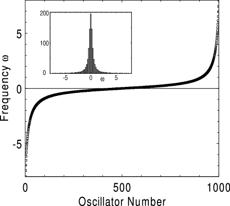
Figure 1: Distribution $g(\omega)$ of frequencies for cutoff Lorentzian with $g(0)=1$ and cutoff $\omega_{c}=8$ for $N=1000$ oscillators. The main graph shows the individual frequencies, and the inset a histogram.

We now show results of numerical simulations for the Lorentzian distribution of frequencies. We have chosen to cut off the distribution at some large $\omega_{c}$ otherwise there would be a few very fast oscillators restricting the time stepping of the numerics. Thus we use

$$g(\omega)=\left\{\begin{tabular}[c]{ll}$g(0)\frac{w^{2}}{\omega^{2}+w^{2}}$&for $\left|\omega\right|<\omega_{c}$\\ $0$&for $\left|\omega\right|>\omega_{c}$\end{tabular}\ \ \ \ \ \ \ \ \ \ \right.$$ (17)

for a given choice of $g(0)$, with $w$ then fixed by the normalization condition

$$2wg(0)\tan^{-1}(\omega_{c}/w)=1\text{.}$$ (18)

(It is useful to parameterize the distribution in terms of $g(0)$, since this quantity determines the values of $\alpha$ and $\beta$ at which synchronization occurs in the large $\alpha\beta$ limit where the model reduces to the Kuramoto phase model Eq. (3).) In presenting the results we choose a distribution width such that $g(0)=1$. For a cutoff $\omega_{c}=8$ this gives $w\simeq(f\pi)^{-1}$, with $f=0.974$. With no cutoff, we would have $f=1$. The distribution of frequencies is generated from a uniform distribution of $N$ values $v_{n}$ on the interval $-\frac{1}{2}<v_{n}<\frac{1}{2}$ using the transformation

$$\omega_{n}=w\tan(\pi fv_{n}).$$ (19)

We present results for a deterministic set of $\nu_{n}$

$$\nu_{n}=\left[n-\frac{1}{2}(N+1)\right]/(N-1),$$ (20)

but have also used $\nu_{n}$ generated randomly on the interval. The distribution of frequencies for $N=1000$ oscillators and a cutoff $\omega_{c}=8$ is shown in Fig. 1.

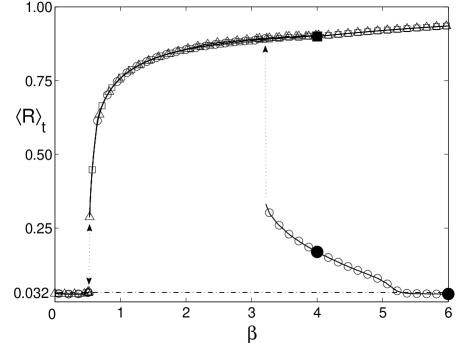
Figure 2: Solutions observed in simulations of $N=1000$ oscillators with the cutoff Lorentzian distribution of intrinsic frequencies of Fig. 1. Shown is the time averaged order parameter magnitude $\langle R\rangle_{t}$ over a range of $\beta$ values at constant $\alpha=1.5$. Solid lines are the observed solutions. The overlapping symbols are representative results from simulations following different solution branches with increasing $\beta$ ($\triangle$) and decreasing $\beta$ ($\Box$ and $\bigcirc$). Time traces associated with the solid symbols are shown in Fig. 3. The dot-dashed line is at a value of $\langle R\rangle_{t}=N^{-1/2}=0.032$, the order of magnitude expected for random fluctuations of the order parameter about zero.

A plot of the dependence of the mean magnitude of the order parameter $\left\langle R\right\rangle_{t}$ as a function of $\beta$ for fixed value of $\alpha=1.5$ and $N=1000$ is shown in Fig. 2. This plot shows three types of states: an unsynchronized state with $\left\langle R\right\rangle_{t}$ essentially zero; and two synchronized states, one with small $\left\langle R\right\rangle_{t}$, growing from $0$ to about $0.3$ as $\beta$ decreases below about $5.2$, and one with large $\left\langle R\right\rangle_{t}$ that exists for all $\beta>0.6$. (We will discuss later such issues as whether the growth of the large $\left\langle R\right\rangle_{t}$ is continuous or discontinuous near $\beta=0.6$.)

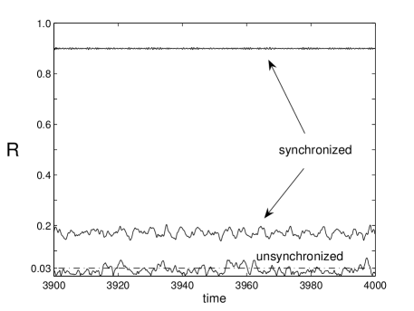
Figure 3: Order parameter magnitude $R$ as a function of time observed at the solid symbols in Fig. 2. The three traces are for the unsynchronized state at $\beta=6.0$ (lower trace), and the small amplitude synchronized state (middle trace) and large amplitude synchronized state (upper trace) both at $\beta=4.0$.

The variation of $R(t)$ for representative examples of these three states is shown in Fig. 3. The lower trace shows the unsynchronized state at $\beta=6.0$ in Fig. 2. The fluctuations in $R(t)$ are consistent with fluctuations of the order parameter about zero with magnitude of order $N^{-1/2}$ as expected for a collection of $N$ oscillators with different frequencies and random phases. The average frequency distribution $\tilde{\omega}_{n}$ (not shown) is unchanged from the bare distribution $\omega_{n}$ shifted by $\alpha+\beta$. This shift can be understood as arising from the nonlinear frequency shift with $\left|z_{n}\right|=1$, and the coupling to a distribution of oscillators with $\left|z_{m}\right|=1$ and random phases.

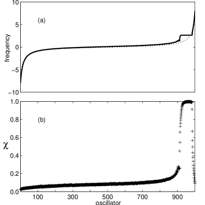
Figure 4: Frequency distribution and synchronization index for the small amplitude synchronized state in Fig. 3: (a) - actual frequency distribution (solid line) and bare frequency distribution shifted by $\alpha+\beta$ (dotted line); (b) - synchronization index $\chi_{n}$.

The state corresponding to the middle trace in Fig. 3 is the low amplitude state at $\beta=4.0$ in Fig. 2. The mean order parameter magnitude $\left\langle R\right\rangle_{t}\simeq 0.17$ is much larger than $N^{-1/2}\simeq.032$, suggesting this is a synchronized state. The corresponding frequency distribution and synchronization index are shown in Fig. 4. The frequency distribution $\tilde{\omega}_{n}$ (a) shows a small plateau of constant frequency over about 60 oscillators towards the high frequency end of the distribution; these are the frequency locked oscillators. The synchronization index (b) shows that $\chi_{n}$ approaches unity for most of the locked oscillators, which means that $z_{n}$ for these oscillators is essentially time independent once the rotation of the phase at the order parameter frequency is subtracted out. A careful scrutiny of the two panels reveals that the plateau in $\tilde{\omega}_{n}$ is sharper and more extended than the one in $\chi_{n}$, so that not all the frequency locked oscillators are time independent in the rotating frame. The dynamical state is actually quite complicated, as a review of $z_{n}(t)$ shows.

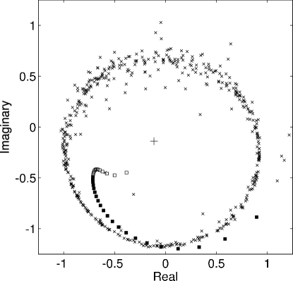
Figure 5: Snapshot of $z_{n}$ and order parameter $\Psi$ in the complex plane at a time after transients have decayed. The “+” towards the center of the plot gives the value of the order parameter. The squares are oscillators locked to the order parameter frequency (i.e. those with $\tilde{\omega}_{n}=\Omega$): solid squares are stationary when the $e^{i{\Omega}t}$ dependence is removed, open squares show an additional dynamics rotating around the tail of the fixed distribution in the rotating system. The “$\times$” are oscillators that are not locked to the order parameter.

Figure 5 shows a plot of a snapshot of the complex amplitude $z_{n}$ of each oscillator. The “+” is the order parameter. The other points correspond to $z_{n}$ for each oscillator. It is useful to study the dynamics of this plot after rotation at the mean order parameter frequency is eliminated. As time evolves, the square symbols remain fixed in such a plot (except for very small fluctuations): these represent oscillators that are locked to the order parameter. For the solid squares the complex amplitudes are essentially time independent once the phase of the order parameter is extracted. The oscillators represented by an “$\times$” on the other hand rotate clockwise or anticlockwise about the origin: these correspond to unlocked or running oscillators. The open squares exhibit a more complicated dynamics undergoing small amplitude orbits around the tail of the locked oscillator distribution. These oscillators are locked to the order parameter, since the difference of their phases from the order parameter phase does not drift over arbitrary long times. The values of $\tilde{\omega}_{n}$ for these oscillators are on the locked plateau in Fig. 4. However the amplitudes are not constant in the rotating plot, the values of $\chi_{n}$ are less than unity, and the oscillators contribute to fluctuations of the order parameter. Thus the fluctuations of $R(t)$ shown in Fig. 3 are not just due to finite $N$ effects, and we believe they would persist in the $N\rightarrow\infty$ limit. We have not explored larger $N$ to pin down whether these intrinsic fluctuations are periodic or aperiodic in the large $N$ limit.

As we discuss in more detail later, for a bounded distribution of frequencies it is possible to find a low amplitude synchronized state with $R\neq 0$, but with a smooth frequency distribution showing that there is no frequency locking. In fact for this state the distribution of actual oscillator frequencies does not overlap the order parameter frequency. The nonzero order parameter is caused by a systematic slowing of the phase rotation of the oscillators in the vicinity of the order parameter phase, rather than by a fraction of the phases becoming locked to the order parameter phase. For an unbounded distribution such as the Lorentzian, this same effect occurs but is supplemented by the small fraction of locked oscillators.

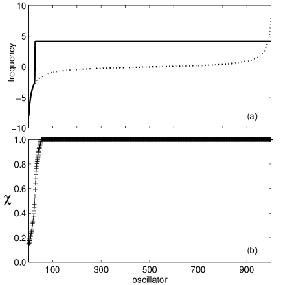
Figure 6: Same as in Fig. 4 but for the large amplitude synchronized state.

For the same parameter values as for the previously described low amplitude synchronized state for the Lorentzian distribution there is a second dynamical state that may be reached depending on the initial conditions of the simulation. This state has a much larger value of the order parameter $\left\langle R\right\rangle_{t}\simeq 0.9$ and the plot of the distribution of frequencies, Fig. 6(a), shows a correspondingly larger fraction of locked oscillators. (This should be compared with panel (a) of Fig. 4.) For the cutoff Lorentzian distribution used, all the oscillators at the high frequency end of the distribution are locked, leaving only a small fraction of free running oscillators at the low end of the frequency distribution. For the $N\rightarrow\infty$ limit and a Lorentzian distribution without a cutoff, unlocked oscillators remain at both the high and low frequency ends of the distribution. For a bounded distribution of bare frequencies, such as triangular or top-hat, a fully locked state in which all the oscillators rotate with the same frequency and fixed magnitude may be found.

IV Formulation of Synchronization

We now turn to the analysis of the synchronization of oscillators described by Eq. (1). Since we are interested in the behavior for a large number of oscillators, it is convenient to go to a continuum description, where we label the oscillators by their uncoupled linear frequency $\omega=\omega_{n}$ rather than the index $n$, $z_{n}\rightarrow z(\omega)$. Introducing the order parameter Eq. (4), the oscillator equations can be written in magnitude-phase form as

$$d_{t}\bar{\theta} =\bar{\omega}+\alpha(1-r^{2})+\frac{\beta R}{r}\cos\bar{\theta}$$ (21a)

$$d_{t}r =(1-r^{2})r+\beta R\sin\bar{\theta}$$ (21b)

where $$\bar{\theta}=\theta-\Theta \bar{\omega} \alpha+\beta \Omega=\dot{\Theta}$$ is the oscillator phase relative to that of the order parameter as before, and is the bare oscillator frequency shifted by and measured relative to the order parameter frequency

$$\bar{\omega}=\omega-\alpha-\beta-\Omega.$$ (22)

Note that if the order parameter is zero $R=0$, the magnitude $r$ will relax to $1$, and the $n$th oscillator will evolve at the frequency $\omega_{n}-\alpha-\beta$. The first component of this frequency shift is just the nonlinear shift at $r=1$, and the second is from the interaction of each oscillator with the incoherent motion of the other oscillators.

At each time $t$ the oscillators are specified by the distribution $\rho(r,\bar{\theta},\bar{\omega},t)$ where $\rho(r,\bar{\theta},\bar{\omega},t)r\,dr\,d\bar{\theta}$ is the fraction of the oscillators with shifted frequency $\bar{\omega}$ that at time $t$ have magnitude between $r$ and $r+dr$ and shifted phase between $\bar{\theta}$ and $\bar{\theta}+d\bar{\theta}$. The order parameter is given by the self-consistency condition

$$R\,=\left\langle re^{i\bar{\theta}}\right\rangle=\int d\bar{\omega}\bar{g}(\bar{\omega})\int r\,dr\,d\bar{\theta}\rho(r,\bar{\theta},\bar{\omega},t)re^{i\bar{\theta}}.\,$$ (23)

where $\bar{g}(\bar{\omega})$ is the distribution of oscillator frequencies expressed in terms of the shifted frequency $\bar{\omega}$. It is useful to split this expression into real and imaginary parts. The imaginary part is

$$\int d\bar{\omega}\bar{g}(\bar{\omega})\int r\,dr\,d\bar{\theta}\rho(r,\bar{\theta},\bar{\omega},t)r\sin\bar{\theta}=0.$$ (24)

Because the phases $\bar{\theta}$ are measured relative to the orientation of the order parameter, this expresses the fact that the components of the complex amplitudes $r\sin\bar{\theta}$ normal to the order parameter must average to zero. Note that unlike the cases of the Kuramoto model [Eq. (3)] and the dissipatively coupled complex amplitude model [Eq. (2)] studied by Matthews et al., this condition is not trivially satisfied even for the case of a symmetric distribution $g(\omega)$, and in fact serves to determine the frequency $\Omega$ of the order parameter. The frequency $\Omega$ is also not trivially related to the mean frequency of the oscillator distribution. The real part of Eq. (23) is

$$\int d\bar{\omega}\bar{g}(\bar{\omega})\int r\,dr\,d\bar{\theta}\rho(r,\bar{\theta},\bar{\omega},t)r\cos\bar{\theta}=R.$$ (25)

This is the condition that the components $r\cos\bar{\theta}$ along the direction of the order parameter must average to the magnitude $R$. This condition serves to self-consistently fix the value of $R$.

The expectation that Eqs. (21) might lead to synchronization follows from the behavior for narrow frequency distributions and large $\alpha$. If the width of the distribution of frequencies is small compared to the relaxation rate of the magnitude, which is of order one in the time units used in Eq. (1), the magnitude relaxes rapidly to the value given by the instantaneous value of $\bar{\theta}$, i.e. to the solution of

$$(1-r^{2})r=-\beta R\sin\bar{\theta}.$$ (26)

If $r$ is close to one, which we will see applies at the onset of synchronization for large $\alpha$, this gives

$$1-r^{2}\simeq-\beta R\sin\bar{\theta}.$$ (27)

In this case Eq. (21a) becomes, ignoring $\beta R$ compared with $\alpha\beta R$,

$$d_{t}\bar{\theta}\simeq\bar{\omega}-\alpha\beta R\sin\bar{\theta}.$$ (28)

This equation is the same as the one derived from the Kuramoto model in Eq. (5) with $\alpha\beta$ playing the role of the coupling constant $K$, and therefore predicts an onset of synchronization at $\alpha\beta=2(\pi g(0))^{-1}$ K75 .

To uncover more fully the behavior of Eq. (1) we consider two issues: the onset of synchronization, detected as the linear instability of the unsynchronized $R=0$ state, as a function of $\alpha$ and $\beta$ for some given frequency distribution $g(\omega)$; and the existence of a fully locked state for large values of $\alpha\beta$.

V Onset of synchronization

We first consider the initial onset of partial synchronization from the unsynchronized state in which each oscillator runs at its own frequency $\omega_{n}$. We identify synchronization through a nonzero value of the order parameter. This often arises because a finite fraction of the oscillators become locked to the same frequency, which we call a partially (fully if the fraction is unity) locked state. However we also find situations where $R\neq 0$, but there is no frequency locking.

The onset of synchronization can be determined by a linear instability analysis of the unsynchronized state. This is calculated by linearizing the distribution $\rho$ around the unsynchronized distribution, which is a uniform phase distribution at $r=1$, and seeking the parameter values at which deviations from the uniform phase distribution begin to grow exponentially. This follows the method of Matthews et al. MMS91 , although care is needed in the analysis due to the more important role the magnitude perturbations $r$ play in the present case.

Introducing the small expansion parameter $\varepsilon$ characterizing the small deviations from the unsynchronized state, we write

$$\rho(r,\theta,\bar{\omega},t)=(2\pi r)^{-1}\delta[r-1-\varepsilon r_{1}(\bar{\theta},\bar{\omega},t)][1+\varepsilon f_{1}(\bar{\theta},\bar{\omega},t)].$$ (29)

Note that for $\varepsilon=0$ this does indeed give the appropriately normalized distribution for the unsynchronized state, in which all the oscillators have unit magnitude, $r=1$, and the phase distribution is constant. Also, for nonzero $\varepsilon$, $\rho$ remains normalized to linear order

$$\int_{0}^{\infty}dr\int_{0}^{2\pi}d\theta\,r\,\rho(r,\theta,\bar{\omega},t)=1+O(\varepsilon^{2}),$$ (30)

providing the average of $f_{1}$ over $\bar{\theta}$ is zero.

The equation for the evolution of the radial perturbation of the distribution $r_{1}$ is given by noting that

$$\frac{dr}{dt}=\frac{\partial r}{\partial\bar{\theta}}d_{t}\bar{\theta}+\frac{\partial r}{\partial t}.$$ (31)

The left hand side is evaluated by expanding Eq. (21b) to first order in $\varepsilon$ and also expanding the magnitude of the order parameter $R=\varepsilon R_{1}+\cdots$. , and the right hand side by the replacement $d_{t}\bar{\theta}=\bar{\omega}+O(\varepsilon)$ and assuming an exponential growth or decay of the perturbation $\partial r/\partial t=\varepsilon\partial r_{1}/\partial t=\lambda\varepsilon r_{1}$. The result is

$$\frac{\partial r_{1}}{\partial\bar{\theta}}\bar{\omega}+(\lambda+2)r_{1}=\beta R_{1}\sin\bar{\theta}.$$ (32)

Equation (32) is solved by

$$r_{1}=R_{1}(A\cos\bar{\theta}+B\sin\bar{\theta}),$$ (33)

with

$$A =-\beta\frac{\bar{\omega}}{\bar{\omega}^{2}+(\lambda+2)^{2}},$$ (34a)

$$B =\beta\frac{(\lambda+2)}{\bar{\omega}^{2}+(\lambda+2)^{2}}.$$ (34b)

To extract the equation for $f_{1}$ integrate the equation for the conservation of probability

$$\frac{\partial\rho}{\partial t}+\mathbf{\nabla}\cdot(\rho\mathbf{v})=0$$ (35)

over radius. Here $\mathbf{v}$ is the velocity in complex amplitude space, which in polar coordinates is $(d_{t}r,rd_{t}\bar{\theta})$ given by Eqs. (21). Again replacing $\partial f_{1}/\partial t$ by $\lambda f_{1}$, and evaluating $r_{1}$ from Eqs. (33,34), this gives at $O(\varepsilon)$

$$\lambda f_{1}+\bar{\omega}\partial_{\bar{\theta}}f_{1}=2\alpha R_{1}(-A\sin\bar{\theta}+B\cos\bar{\theta})+\beta R_{1}\sin\bar{\theta}.$$ (36)

This is solved by

$$f_{1}=R_{1}(C\cos\bar{\theta}+D\sin\bar{\theta})$$ (37)

with

$$C =\beta\frac{2\alpha(\lambda^{2}+2\lambda-\bar{\omega}^{2})-\bar{\omega}[\bar{\omega}^{2}+(\lambda+2)^{2}]}{\left(\bar{\omega}^{2}+\lambda^{2}\right)\left[\bar{\omega}^{2}+(\lambda+2)^{2}\right]},$$ (38a)

$$D =\beta\frac{4\alpha\bar{\omega}(\lambda+1)+\lambda[\bar{\omega}^{2}+(\lambda+2)^{2}]}{\left(\bar{\omega}^{2}+\lambda^{2}\right)\left[\bar{\omega}^{2}+(\lambda+2)^{2}\right]}.$$ (38b)

We now evaluate the self-consistency condition Eq. (23) to first order in $\varepsilon$. The imaginary part is

$$\int d\bar{\omega}\,\bar{g}(\bar{\omega})\int_{0}^{2\pi}d\bar{\theta}\,(1+\varepsilon r_{1}+\cdots)(1+\varepsilon f_{1}+\cdots)\sin\bar{\theta}=0,$$ (39)

which to first order in $\varepsilon$ gives

$$\int d\bar{\omega}\,\bar{g}(\bar{\omega})\left[B+D\right]=0.$$ (40)

Similarly the real part of the self-consistency condition is

$$\int d\bar{\omega}\,\bar{g}(\bar{\omega})\left[A+C\right]=2.$$ (41)

We want to evaluate Eqs. (40) and (41) at the onset of instability where the growth rate $\lambda\rightarrow 0$. We can set $\lambda=0$ in Eqs. (40,41) with Eqs. (34) and (38) except in terms with $\bar{\omega}^{2}+\lambda^{2}$ in the denominator, since such terms may give large contributions to the integral from the region of small $\bar{\omega}$. A term involving just $\lambda/(\bar{\omega}^{2}+\lambda^{2})$ gives a finite integral, but if this is multiplied by powers of $\bar{\omega}$ or $\lambda$ the integral goes to zero in the $\lambda\rightarrow 0$ limit. Similarly for a term involving $\bar{\omega}/(\bar{\omega}^{2}+\lambda^{2})$ we must take the limit $\lambda\rightarrow 0$ after doing the integral (this is equivalent to the principal value integral), whereas if this term is multiplied by powers of $\bar{\omega}$ we can put $\lambda=0$ immediately.

The needed integrals are

$$I_{1} =\int\bar{g}(\bar{\omega})\frac{1}{\bar{\omega}^{2}+4},$$ (42a)

$$I_{2} =\lim_{\lambda\rightarrow 0}\int\bar{g}(\bar{\omega})\frac{\bar{\omega}}{\bar{\omega}^{2}+\lambda^{2}},$$ (42b)

$$I_{3} =\int\bar{g}(\bar{\omega})\frac{\bar{\omega}}{\bar{\omega}^{2}+4},$$ (42c)

$$I_{4} =\lim_{\lambda\rightarrow 0}\int\bar{g}(\bar{\omega})\frac{\lambda}{\bar{\omega}^{2}+\lambda^{2}}=\pi\bar{g}(\bar{\omega}=0).$$ (42d)

The imaginary part of the self consistency condition Eq. (40) becomes

$$2I_{1}+\alpha I_{2}-\alpha I_{3}+I_{4}=0,$$ (43)

and the real part reduces to the condition for $\beta_{c}$

$$\beta_{c}=2(-I_{3}+\alpha I_{4}-2\alpha I_{1}-I_{2})^{-1}.$$ (44)

We have explicitly evaluated the integrals for top-hat, triangular, and Lorentzian distributions of bare frequencies. These results will be presented after we discuss full locking.

VI Full Locking

We define the fully locked state as one in which all the phases are rotating at the same frequency as the order parameter, and the magnitudes are constant in time. These solutions are defined by Eq. (21a) with $d_{t}\bar{\theta}=0$, which with Eq. (26) can be written

$$\bar{\omega}=\frac{\beta R}{r}(\alpha\sin\bar{\theta}-\cos\bar{\theta})=F(\bar{\theta}),$$ (45)

where the solution to the cubic equation (26) for $r(\bar{\theta})$ is to be used to form the function of phase alone $F(\bar{\theta})$. The function $F(\bar{\theta})$ acts as the force pinning the locked oscillators to the order parameter, generalizing the notion introduced below Eq. (5), and plays a central role in our discussion of locking. A particular oscillator, identified by its shifted frequency $\bar{\omega}$, will be locked to the order parameter if Eq. (45) has a solution $\bar{\theta}=F^{-1}(\bar{\omega})$ [and then $r$ is given by solving Eq. (26)] and if this solution is stable. The stability is tested by linearizing Eqs. (21) about the solution. The fully locked solution will only exist if stable, locked solutions to Eq. (45) exist for all the oscillators in the distribution. We are thus led to investigate the properties of the function $F(\bar{\theta})$. In addition the self consistency condition Eq. (23) must be satisfied.

For small $\beta R$, the magnitude $r(\bar{\theta})$ given by Eq. (26) remains bounded away from zero for all $\bar{\theta}$, and the function $F(\bar{\theta})$ varies continuously between minimum and maximum values $F_{\min}\leq F\leq F_{\max}$. In this case, we immediately see that the fully locked solution only occurs for bounded distributions, $\bar{g}(\bar{\omega})$ nonzero only between finite $\bar{\omega}_{\min}$ and $\bar{\omega}_{\max}$. In such cases we define $\bar{\omega}_{\max}-\bar{\omega}_{\min}$, which is equal to the range of unshifted frequencies $\omega_{\max}-\omega_{\min}$, as $w$ the width of the distribution. More generally, although $F(\bar{\theta})$ can vary over an infinite range (because $r$ may become zero) we find that only a finite range yields stable solutions, so that again complete locking only occurs for a bounded distribution of oscillator frequencies.

We first look at the fully locked solution for large values of $\alpha\beta$. In this case the phases of the locked oscillators cover a narrow range of angles, since the range of the pinning force $F$ becomes large for large $\alpha\beta$. The imaginary part of the self consistency condition Eq. (24) shows that the range of phases must be around $\bar{\theta}=0$. Equation (45) can now be approximated by expanding around $\bar{\theta}=0$ (note $r\simeq 1$ here) and becomes for large $\alpha$

$$\bar{\omega}=\omega-\alpha-\beta-\Omega\simeq-\beta R(1-\alpha\bar{\theta}).$$ (46)

The imaginary part of the self-consistency condition reduces to $\left\langle\bar{\theta}\right\rangle=0$ (the average is over the distribution of frequencies), and the real part to simply $R\simeq 1$. Finally, averaging Eq. (46) over the distribution of frequencies fixes the order parameter frequency (the common frequency of all the oscillators)

$$\Omega\simeq\left\langle\omega\right\rangle-\alpha.$$ (47)

Thus the order parameter, and all the oscillators, evolve at a frequency given by the mean of the distribution $g(\omega)$ shifted by the nonlinear effect for $r=1$.

We now investigate the limit to the fully locked regime as we lower $\alpha$. We first summarize the argument, and then present the details. The fully locked solutions are determined by a rather complicated set of interconnected equations. They can be found by the following algorithm. For fixed values of $\alpha,B=\beta R$ solve Eq. (26) for real positive $r(\bar{\theta})$ and hence calculate $F(\bar{\theta})$. Using Eqs. (21) the stability of each solution is tested: the eigenvalues of this analysis are (see Eq. (60) below)

$$\lambda_{\pm}=1-2r^{2}\pm\sqrt{1-\frac{B^{2}}{r^{2}}-2r^{2}+2r^{4}-2\alpha rB\cos\bar{\theta}},$$ (48)

with $\cos\bar{\theta}=\pm\sqrt{1-r^{2}(1-r^{2})^{2}/B^{2}}$. From this we can identify a range $F_{\min}^{(s)}<F<F_{\max}^{(s)}$ corresponding to the range of existence and stability of locked oscillators. A fully locked solution must then satisfy the constraints

$$\bar{\omega}_{\min}\geq F_{\min}^{(s)};~{}\bar{\omega}_{\max}\leq F_{\max}^{(s)},$$ (49)

together with the condition given by the imaginary part of the self consistency condition

$$\int_{\bar{\omega}_{\min}}^{\bar{\omega}_{\max}}\bar{g}(\bar{\omega})\,r(\bar{\omega})\sin[\bar{\theta}(\bar{\omega})]\,d\bar{\omega}=0,$$ (50)

where $\bar{\theta}(\bar{\omega})=F^{-1}(\bar{\omega})$, and $r(\bar{\omega})$ is then the solution to Eq. (26). The boundary of the fully locked region occurs either when $\bar{\omega}_{\min}=F_{\min}^{(s)}$ or when $\bar{\omega}_{\max}=F_{\max}^{(s)}$. This equation can be interpreted as fixing the order parameter frequency $\Omega$ in terms of $\alpha$ and $B$. Notice that Eq. (48) shows that for $r<1/\sqrt{2}$ one eigenvalue certainly has a positive real part indicating instability, so that for stable solutions $r\geq 1/\sqrt{2}$ and $F_{\min}^{(s)}$ is finite. Since $\bar{\omega}_{\min}$ or $\bar{\omega}_{\max}$ is now determined, and $\bar{\omega}_{\max}-\bar{\omega}_{\min}=w$, Eq. (50) is an implicit equation relating the values of $\alpha$, $B$ and $w$ at the locking transition. To complete the solution, the real part of the self consistency equation

$$\int_{\bar{\omega}_{\min}}^{\bar{\omega}_{\max}}\bar{g}(\bar{\omega})\,r(\bar{\omega})\cos[\bar{\theta}(\bar{\omega})]\,d\bar{\omega}=R$$ (51)

then serves to fix $R$ at locking, from which the value of $\beta=B/R$ at the transition to full locking can be found.

VI.1 Existence of individual oscillator locked solution

We first consider the existence of a locked solution for an individual oscillator, i.e. a stationary solution of Eqs. (21). Equation (26) gives the cubic equation for $r(\bar{\theta})$ for each $B=\beta R$

$$(1-r^{2})r+B\sin\bar{\theta}=0.$$ (52)

Of course, for the physical solution $r$ must be real and positive. Thus we need to analyze the properties of the real positive solutions to

$$(1-r^{2})r+X=0,$$ (53)

as $X$ varies.

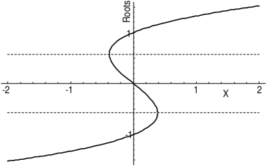
Figure 7: Solutions to the cubic equation Eq. (53) as $X$ varies. The dashed lines are $y=\pm 1/\sqrt{3}$.

For $X=0$ the solutions to the cubic are $r=\pm 1,0$. As $\left|X\right|$ increases, the solutions remain real until two of the roots collide and become complex. Since the sum of the roots to Eq. (53) is zero, at the collision the equation takes the form

$$(r-a)^{2}(r+2a)=0.$$ (54)

Matching coefficients shows that collision occurs at $X=\pm\frac{2}{\sqrt{27}}$ when $r=\mp\frac{1}{\sqrt{3}}$. The form of Eq. (53) is actually already in what is known as the “depressed form” of a cubic equation, for which the solution is relatively simple. Inspecting the form of these solutions shows that for $\left|X\right|>\frac{2}{\sqrt{27}}$ there is one real solution and a complex pair in the form $2a,-a\pm ib$. The product of the roots is determined by the constant in the cubic, giving

$$2a(a^{2}+b^{2})=X$$ (55)

and so for $X<-\frac{2}{\sqrt{27}}$ the real root is negative, and for $X>\frac{2}{\sqrt{27}}$ the real root is positive. These results are confirmed by numerical solution as shown in Fig. 7.

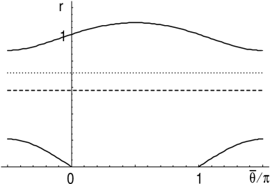
Figure 8: Plot of $r(\bar{\theta})$ for $B<2/\sqrt{27}$. The dashed line is $r=1/\sqrt{3}$ and the dotted line $r=1/\sqrt{2}$. The condition $r>1/\sqrt{2}$ is necessary (but not sufficient) for the solution to be stable. The lower branch always satisfies $r<1/\sqrt{3}$, and so only the upper branch may have stable regions.

Figure 9: Plot of $r(\bar{\theta})$ for $B>2/\sqrt{27}$. Solutions exist for $-\theta_{B}\leq\bar{\theta}\leq\pi+\theta_{B}$ with $\theta_{B}=\sin^{-1}(2/B\sqrt{27})$. The dashed line is $r=1/\sqrt{3}$ and the dotted line $r=1/\sqrt{2}$.

Thus we find the following behavior for the real positive solutions to Eq. (52). For $B<2/\sqrt{27}$ there is a root that is positive with $r>1/\sqrt{3}$ for all $\bar{\theta}$, a root that varies between positive and negative values with magnitude less than $1/\sqrt{3}$, and a root that is negative for all $\bar{\theta}$. We have seen that the stability analysis shows that any solution with $r<1/\sqrt{2}$ is unstable. Thus only the first root is relevant (see Fig. 8). For $B>2/\sqrt{27}$ real positive roots exist for $-\theta_{B}\leq\bar{\theta}\leq\pi+\theta_{B}$ with $\theta_{B}=\sin^{-1}\frac{2}{B\sqrt{27}}$. In the range where there are two real positive roots, $-\theta_{B}\leq\bar{\theta}\leq 0$ and $\pi\leq\bar{\theta}\leq\pi+\theta_{B}$, only the larger may be in the stable range $r>1/\sqrt{2}$, (see Fig. 9).

Having found the stationary solutions $r(\bar{\theta})$, the condition for stationary phase $d_{t}\bar{\theta}=0$ can be written

$$\bar{\omega}=F(\bar{\theta})$$ (56)

with

$$F(\bar{\theta})=\frac{\beta R}{r(\bar{\theta})}(\alpha\sin\bar{\theta}-\cos\bar{\theta}).$$ (57)

The function $F(\bar{\theta})$ acts as the force acting on each oscillator tending to pin its frequency to the order parameter frequency. The range of possible $\bar{\omega}$ for locked oscillators is limited by the range of $F$ corresponding to stable stationary solutions.

VI.2 Stability of individual oscillator locked solution

The stability of the locked solution for an individual oscillator mentioned in the previous section is given by linearizing Eqs. (21) about the stationary solutions. The linearized equations are

$$d_{t}\delta\bar{\theta} =-\left(\frac{\beta R}{r}\sin\bar{\theta}\right)\,\delta\bar{\theta}-\left(2\alpha r+\frac{\beta R}{r^{2}}\cos\bar{\theta}\right)\delta r$$ (58)

$$d_{t}\delta r =(\beta R\cos\bar{\theta})\,\delta\bar{\theta}+(1-3r^{2})\delta r$$ (59)

The eigenvalues are

$$\lambda_{\pm}=1-2r^{2}\pm\sqrt{S}$$ (60)

with

$$S=1-\frac{B^{2}}{r^{2}}-2r^{2}+2r^{4}-2\alpha Br\cos\bar{\theta}$$ (61)

This immediately shows us $r>1/\sqrt{2}$ is a necessary condition for stability, since $\operatorname{Re}\lambda_{+}\geq 1-2r^{2}$ (with the equality if $S$ is negative so that $\lambda_{\pm}$ are complex).

Let us first seek the condition for a root $\lambda_{\pm}$ to become zero, signaling a stationary bifurcation. It is convenient to go back to the original equations Eqs. (21) in the form

$$d_{t}\bar{\theta} =\bar{\omega}-f(r,\bar{\theta})$$ (62a)

$$d_{t}r =(1-r^{2})r+\beta R\sin\bar{\theta}$$ (62b)

with

$$f(r,\bar{\theta})=-\alpha(1-r^{2})-\frac{\beta R}{r}\cos\bar{\theta}.$$ (63)

Then the determinant of the linear matrix derived from Eqs. (62) is

$$D=\left|\begin{array}[c]{cc}-\frac{\partial f}{\partial\bar{\theta}}&-\frac{\partial f}{\partial r}\\ \beta R\cos\bar{\theta}&1-3r^{2}\end{array}\right|=-(1-3r^{2})\frac{\partial f}{\partial\bar{\theta}}+\beta R\cos\bar{\theta}\frac{\partial f}{\partial r}.$$ (64)

The stationary solution $r(\bar{\theta})$ satisfies Eq. (52) and so Eq. (64) can be written

$$D=-(1-3r^{2})\frac{dF}{d\bar{\theta}},$$ (65)

since

$$\frac{dF(\bar{\theta})}{d\bar{\theta}}=\frac{df(\bar{\theta},r(\bar{\theta}))}{d\bar{\theta}}=\frac{\partial f}{\partial\bar{\theta}}+\frac{\partial f}{\partial r}\frac{dr}{d\bar{\theta}}.$$ (66)

Thus a zero eigenvalue occurs at and only at stationary points of $F(\bar{\theta})$ or at $r=1/\sqrt{3}$. The latter is where $r(\bar{\theta})$ has a vertical tangent (cf. Fig. 9) but always occurs outside the range of stable solutions, for which we know $r>1/\sqrt{2}$.

The only other possibility for an instability is $\operatorname{Re}\lambda_{\pm}=0$, $\operatorname{Im}\lambda_{\pm}\neq 0$. This can occur only at $r=1/\sqrt{2}$, and if $S<0$.

Another result can be derived: if $dF/d\bar{\theta}<0$ and $r>1/\sqrt{3}$ then the determinant $D<0$. This implies that the eigenvalues are real (since the product of a complex conjugate pair is always positive), one positive and one negative. Thus a negative slope of $F(\bar{\theta})$ implies instability. Also the Hopf bifurcation can only occur at values of $\bar{\theta}$ where $dF/d\bar{\theta}>0$.

To satisfy the imaginary part of the self-consistency condition Eq. (50), the range of phases of locked oscillator phases must straddle $\bar{\theta}=0$. The oscillator solution here, $\bar{\theta}=0,r=1$ is always stable for positive $\alpha,B$, since here $\lambda_{+}=-1+\sqrt{1-B(B+2\alpha)}$. Thus the range of possible stable stationary solutions for locked oscillators is given by the range of $\bar{\theta}$ bounded on either side of $\bar{\theta}=0$ by the closest stationary bifurcation point or by a Hopf bifurcation occurring at $r=1/\sqrt{2}$, whichever is closest.

VI.3 Properties of the locking force

We now derive the properties of the locking force, $F(\bar{\theta})$. For small $B=\beta R$, Eq. (26) yields a stationary solution with $r(\bar{\theta})\simeq 1$ and so

$$F(\bar{\theta}) \simeq B(\alpha\sin\bar{\theta}-\cos\bar{\theta})$$ (67)

$$=B\sqrt{\alpha^{2}+1}\sin(\bar{\theta}-\theta_{\alpha})$$ (68)

with $\theta_{a}=\tan^{-1}(1/\alpha)$. Thus $F(\bar{\theta})$ is a sinusoidal function of angle in this limit. The stable solutions are the positive slope region for $\bar{\theta}$ between $\theta_{\alpha}-\pi/2$ and $\theta_{\alpha}+\pi/2$.

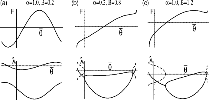
Figure 10: Behavior of the locking force $F(\bar{\theta})$ and the stability eigenvalues $\lambda_{\pm}$ for (a) $\alpha=1.0,B=0.2$, (b) $\alpha=0.2,B=0.8$, and (c) $\alpha=1.0,B=1.2$. The range of angles plotted is $\bar{\theta}$ between $-\pi/2$ and $3\pi/2$ for $B<2/\sqrt{27}$, panel (a), and between $-\bar{\theta}_{B}$ and $\pi+\bar{\theta}_{B}$ for $B>2/\sqrt{27}$, panels (b) and (c). In the eigenvalue plots the solid curves are $\operatorname{Re}\lambda_{\pm}$ and the dashed curves $\operatorname{Im}\lambda_{\pm}$.

As $B$ increases, the behavior becomes quite complicated, and we have not succeeded in proving any results about the full range of possible behavior of $F(\bar{\theta})$. Some examples are shown in Fig. 10. For $B<2/\sqrt{27}$ we have not uncovered parameters leading to an $F$-curve qualitatively different from that in panel (a), i.e. a single maximum and minimum. Note however, that for $B>1/\sqrt{8}$ values of $r<1/\sqrt{2}$ are encountered, and so the Hopf bifurcation may limit the range of stable solutions moving away from $\bar{\theta}=0$, before the maximum or minimum of $F$ is reached. For $B>2/\sqrt{27}$ the physical solutions are limited to the range $-\theta_{B}\leq\bar{\theta}\leq\pi+\theta_{B}$, and the slope of $r(\bar{\theta})$ diverges at the end points: $dr/d\bar{\theta}\rightarrow\infty$ for $\theta\rightarrow-\theta_{B}$ and $dr/d\bar{\theta}\rightarrow-\infty$ for $\theta\rightarrow\pi+\theta_{B}$. Since

$$\frac{dF}{d\bar{\theta}}=-\frac{B}{r^{2}}\frac{dr}{d\bar{\theta}}(\alpha\sin\bar{\theta}-\cos\bar{\theta})+\frac{B}{r}(\alpha\cos\bar{\theta}+\sin\bar{\theta})$$ (69)

we see that when $\left|dr/d\bar{\theta}\right|\rightarrow\infty$

$$\frac{dF}{d\bar{\theta}}\rightarrow-\frac{F}{r}\frac{dr}{d\bar{\theta}}$$ (70)

so that $dF/d\bar{\theta}\rightarrow\pm\infty$ with the sign given by the sign of $F$ for $\bar{\theta}\rightarrow\pi+\theta_{B}$ (where $dr/d\bar{\theta}<0$) and opposite to the sign of $F$ for $\bar{\theta}\rightarrow-\theta_{B}$ (where $dr/d\bar{\theta}>0$). This shows, for example, that for the parameters such as those in panel (c) of Fig. 10 where $F(\bar{\theta}\rightarrow\pi+\theta_{B})>0$, the slope $dF/d\bar{\theta}$ approaches $+\infty$ as $\bar{\theta}\rightarrow\pi+\theta_{B}$. This implies that either there is an additional minimum between the maximum of $F$ and $\bar{\theta}\rightarrow\pi+\theta_{B}$ as in this panel, or the maximum disappears and $F(\bar{\theta})$ becomes monotonically increasing in this region, as for the parameters in panel (b). On the other hand for $\alpha=1,B=0.5$, parameters between those of panels (a) and (c), it turns out that $F(\pi+\theta_{B})<0$, so that $dF/d\bar{\theta}\rightarrow-\infty$ as $\bar{\theta}\rightarrow\pi+\theta_{B}$, and $F(\bar{\theta})$ may decrease monotonically between the maximum and $\bar{\theta}\rightarrow\pi+\theta_{B}$.

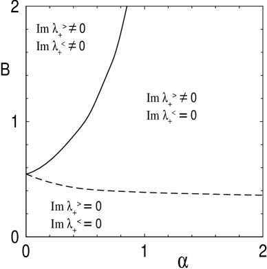
Figure 11: Regions of Hopf bifurcation ($\operatorname{Im}\lambda_{+}\neq 0$) for the first instability of the locked oscillator solution either side of $\bar{\theta}=0.$ For $\bar{\theta}<0$ the value of $\operatorname{Im}\lambda_{+}$ is nonzero above the dashed curve, and for $\bar{\theta}>0$ it is nonzero above the solid curve.

In Fig. 11 the regions where the first instability on either side of $\bar{\theta}=0$ is a Hopf bifurcation ($\operatorname{Im}\lambda_{+}^{\lessgtr}\neq 0$ when $\operatorname{Re}\lambda_{+}^{\lessgtr}=0$, with $\lambda_{+}^{<}$ the eigenvalue with larger real value for $\bar{\theta}<0$, and $\lambda_{+}^{>}$ for $\bar{\theta}>0$) are plotted as a function of $\alpha$ and $B$. Note that there may be discontinuous jumps from $\operatorname{Im}\lambda_{+}=0$ to a finite nonzero value of $\operatorname{Im}\lambda_{+}$: for example on the negative $\bar{\theta}$ side, the minimum in $F$, giving a stationary bifurcation, may disappear by colliding with the maximum, and then the first instability jumps to the Hopf bifurcation that was previously not the closest bifurcation to $\bar{\theta}=0$. Figure 11 does not tell the whole story about whether the boundary of the locked state is a stationary or Hopf bifurcation, because in general only the instability on one side of $\bar{\theta}=0$ determines the boundary, and which side this is depends on the distribution of oscillator frequencies via the transverse self-consistency condition. This is considered further below.

VI.4 Self consistency condition

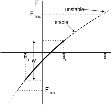
Figure 12: Schematic of transverse self consistency condition, showing the locking force $F(\theta)$ acting on each oscillator as a function of the phase relative to the order parameter $\theta$. The dashed portions of the curve correspond to stable solutions, and the dotted to unstable. The thick solid portion denotes the distribution of oscillator frequencies that must be placed on the stable portion of $F$ and must also satisfy the transverse consistency condition.

We have found a range of $\bar{\theta}$ straddling $\bar{\theta}=0$ giving stable locked solutions for individual oscillators. For a fully locked solution, all the oscillators must have solutions to Eq. (56) in this range. In addition the imaginary part of the self consistency condition Eq. (24) must be satisfied. This can be written in the form

$$\int\bar{g}(\bar{\omega})\,r(\bar{\omega})\sin[\bar{\theta}(\bar{\omega})]\,d\bar{\omega}=0,$$ (71)

since now there is a unique $\bar{\theta}$ and $r$ for each oscillator frequency. Changing the integration variable in Eq. (71) to the angle $\bar{\theta}$ yields

$$\int\bar{g}(F(\bar{\theta}))\,r(\bar{\theta})\sin\bar{\theta}\left|\frac{dF}{d\bar{\theta}}\right|\,d\bar{\theta}=0.$$ (72)

The degree of freedom, for fixed $\alpha,B$ and width of frequency distribution $w$, to be determined by this condition is the order parameter frequency $\Omega$. The scheme of imposing the condition is sketched in Fig. 12. The thick solid line, of fixed length $w$ along the $F$ axis, is to be slid along the curve $F(\bar{\theta})$ (corresponding to varying $\Omega$) until the integral Eq. (72) is zero. All quantities, except $\sin\bar{\theta}$ are positive, and so this line must straddle the origin. This must be done with all of the solid line lying within the stable (dashed) range of $F(\bar{\theta})$.

For a bounded frequency distribution we can always find a fully locked solution for large enough $\alpha\beta$. The argument is as follows. First, there is always a range of stable locked oscillator solutions straddling $\bar{\theta}=0$. If we define $\omega=0$ as the center of the distribution $g(\omega)$ then the order parameter frequency is given by

$$\Omega=-F_{c}-\alpha-B$$ (73)

where $F_{c}$ is $F(\bar{\theta})$ evaluated at the center (with respect to the ordinate) of the solid portion of the curve in Fig. 12, once Eq. (72) is satisfied. Since it follows from Eqs. (57) and (26) that the slope of $F(\bar{\theta})$ at $\bar{\theta}=0$ is

$$F^{\prime}(0)=B(\alpha+B/2),$$ (74)

the range of phase angles of the locked oscillators of order $w/F^{\prime}(0)$ is small for large enough $B$ or $\alpha B$, and there is always a fully locked solution for a bounded frequency distribution in this limit. The center of the band can then be evaluated as $\omega=0$, and so

$$\Omega=-F(0)-\alpha-B.$$ (75)

Also, in this limit all the oscillators have essentially the same phase, so that $R=1$ and $\beta=B$. This gives the complete solution for the fully locked state for very large $\beta$.

It is easiest to understand the limit of the fully locked solution by decreasing $B$ at fixed $\alpha,w$. As $B$ decreases, the range of the locking force $F$ decreases. We can continue to construct the solution as in Fig. 12, with the portion of the $F(\bar{\theta})$ covered by the locked oscillators determined by the transverse self consistency condition, until the first value $B=B_{c}$ is reached for which either the lower end of the locked band would pass below $F_{\min}^{(s)}$, or the upper end of the locked band would pass beyond $F_{\max}^{(s)}$. This signals the onset of instability of the corresponding locked oscillator, either by a stationary or Hopf bifurcation depending on $\operatorname{Im}\lambda_{+}$ at the appropriate $F_{\min}$ or $F_{\max}$ .

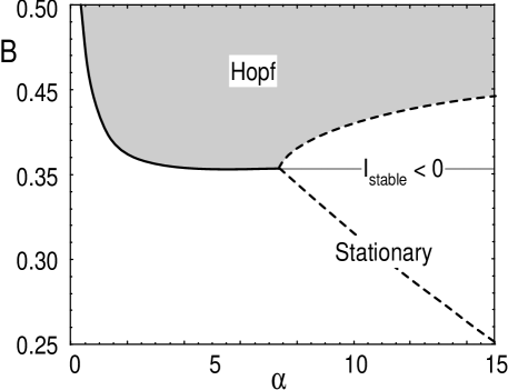
Figure 13: Plot showing regions in the $B-\alpha$ plane for which the instability from the fully locked state is Hopf (shaded) or stationary (unshaded) for a top-hat distribution. The dashed line shows the range of $\alpha,B$ for which $I_{\mathrm{stable}}<0$ for a top-hat distribution. (Note the change of range of $\alpha,B$ plotted compared with Fig. 11.)

We could also imagine increasing the width of the distribution $w$ from the fully locked solution which occurs at small $w$ for fixed $\alpha$ and $B$, until one end of the growing band of locked oscillator solutions reaches $F_{\min}$ or $F_{\max}$. For a top-hat distribution of oscillator frequencies the integral

$$I_{\mathrm{stable}}=\int_{\mathrm{stable}}\bar{g}(F(\bar{\theta}))\,r(\bar{\theta})\sin\bar{\theta}\left|\frac{dF}{d\bar{\theta}}\right|\,d\bar{\theta},$$ (76)

where the integration extends over the whole stable range of $\bar{\theta}$, provides an indicator of whether the limit is reached at the lower or upper bound of the stable band: if $I_{\mathrm{stable}}$ is positive, then to satisfy Eq. (72) the integral must be reduced by lowering the upper integration bound, and so the range of integration extends from the lower stability bound. This gives the condition for the maximum $w$

$$w_{c}/2=F_{c}-F_{\min}^{(s)},$$ (77)

with $F_{\min}^{(s)}$ the lowest $F$ for stable solutions and $F_{c}$ the value of $F$ at the center of the band for $I_{\mathrm{stable}}=0$. On the other hand if $I_{\mathrm{stable}}$ is negative, then the integral Eq. (72) must be increased by raising the lower integration bound, and so the range of integration extends to the upper stability bound. This gives the condition

$$w_{c}/2=F_{\max}^{(s)}-F_{c},$$ (78)

with $F_{\max}^{(s)}$ the largest $F$ for stable solutions. We can then find the range of $\alpha,B$ for which the locked state disappears by a Hopf or by a stationary bifurcation, Fig. 13. This is constructed from Fig. 11, giving the conditions for the instabilities at $F_{\min}^{(s)}$ and $F_{\max}^{(s)}$ to be Hopf or stationary, and the result just determined for which of these instabilities limits the range of the fully locked solution. Numerical results show that for the top-hat distribution the condition $I_{\mathrm{stable}}<0$ occurs only for a restricted range of parameters: large $\alpha$ and $B$ near $2/\sqrt{27}$, the region to the right of the dashed line in Fig. 13. Combining these results yields a Hopf bifurcation from the fully locked state in the shaded region of Fig. 13. For other oscillator distribution shapes we do not have a criterion for the nature of the instability without a detailed solution of the self consistency condition for each width.

So far the solution has been developed in terms of $\alpha,B$. We now determine the magnitude $R$ of the order parameter from the parallel self-consistency condition, the real part of Eq. (23) which can be written in the form

$$\int_{\bar{\theta}_{b}}^{\bar{\theta}_{e}}\bar{g}(F(\bar{\theta}))\,r(\bar{\theta})\cos\bar{\theta}\left|\frac{dF}{d\bar{\theta}}\right|\,d\bar{\theta}=R,$$ (79)

where the range of integration is that determined from the transverse self-consistency condition, see Fig. 12. From $R(\alpha,B)$ we can calculate $\beta=B/R$ at the boundary of locked solutions. If the dependence $R(B)$ is smooth and monotonic, we can map the results depending on $(\alpha,B)$ onto functions of $(\alpha,\beta).$ However, discontinuities in $R(B)$ might well occur due to the jumps in the stability range, for example when the stationary bifurcation disappears as described before. This might lead to values of $\beta$ for which no prediction, e.g. for $w_{c}(\alpha,\beta)$, has been yielded by the algorithm. We do not have results for such cases.

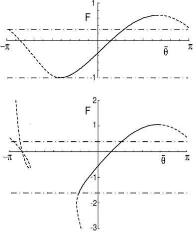
Figure 14: Plots of $F(\bar{\theta})$ for $\alpha=2$, $B=0.34$, $w=1.3$ (top panel), and $\alpha=2$, $B=0.56$, $w=2$ (lower panel) corresponding to the boundary of the fully locked solution: solid curve - stable solutions; dashed curve - unstable solutions. The dash-dotted lines straddle the range of $\bar{\omega}=F(\bar{\theta})$ of locked oscillators, between $F_{\min}$ and $F_{\min}+w$. The values of the order parameter are 0.92 (upper panel) and 0.93 (lower panel).

Two examples of the construction of locked solutions for the triangular distribution, defined below in Eqs. (95), are shown in Fig. 14: the first for small $B=\beta R$, where a solution $r(\bar{\theta})$ exists for all $\bar{\theta}$; and the second for larger $B$ where there are ranges of $\bar{\theta}$ for which no physical solution for the magnitude (i.e. real and positive) exists. The value of $B$ for which Eq. (50) is satisfied in each case was found by simple bisection applied to the numerical results of the integration. In both the cases shown the boundary of the fully locked region occurs when $\bar{\omega}_{\min}=F_{\min}^{(s)}$. For the smaller value of $B$ this condition corresponds to the limit of the existence range of solutions. For the larger value of $B$ the limit occurs at the instability of the locked oscillator solution, which develops via a Hopf bifurcation ($\operatorname{Im}\lambda_{+}\neq 0$). Results for the boundary of the fully locked state for a top-hat distribution with $g(0)=1$ are shown in Fig. 19, and for the triangular distribution with $g(0)=1$ in Fig. 22.

VII Results for various frequency distributions

VII.1 Lorentzian Distribution

In this section we present detailed results for the case of a Lorentzian distribution of frequencies. We concentrate on a distribution with $g(0)=1$, but also present some results for a wider distribution $g(0)=\frac{1}{2}$, which shows some novel features. We begin this section by calculating the linear stability of the unsynchronized state. Since the Lorentzian distribution is unbounded, there is no fully locked solution.

For the purposes of analysis we choose, without loss of generality, a Lorentzian distribution $g(\omega)$ centered about zero frequency

$$g(\omega)=g(0)\frac{w^{2}}{\omega^{2}+w^{2}}\qquad\text{with}\qquad w=(\pi g(0))^{-1}.$$ (80)

The half width at half height is $w$. In terms of the shifted frequency $\bar{\omega}$ the distribution is

$$\bar{g}(\bar{\omega})=g(0)\frac{w^{2}}{(\bar{\omega}+\delta)^{2}+w^{2}},$$ (81)

with

$$\delta=\alpha+\beta+\Omega.$$ (82)

The integrals Eqs. (42) are

$$I_{1} =\frac{2+w}{2(4+4w+w^{2}+\delta^{2})},$$ (83a)

$$I_{2} =\frac{\delta}{w^{2}+\delta^{2}},$$ (83b)

$$I_{3} =\frac{\delta}{4+4w+w^{2}+\delta^{2}},$$ (83c)

$$I_{4} =\frac{w}{w^{2}+\delta^{2}}.$$ (83d)

The imaginary part of the self consistency condition Eq. (43) reduces to

$$\delta^{2}-2\alpha\delta+2w+w^{2}=0.$$ (84)

This serves to fix the frequency of the order parameter $\Omega$ at the onset of synchronization via Eq. (82) in terms of the parameters of the system $\alpha,\beta,w$. There are two solutions for $\delta$

$$\delta=\alpha\pm\sqrt{\alpha^{2}-(2w+w^{2})}.$$ (85)

For large $\alpha$ or small $w$ the approximate solutions are $\delta\simeq(w+\frac{1}{2}w^{2})/\alpha$ giving a locking frequency near the center of the band of the free running oscillators, and $\delta\simeq 2\alpha$ giving a locking frequency far in the tails. Note that the requirement that $\delta$ is real means that $\alpha$ must be sufficiently large $\left|\alpha\right|>\alpha_{\min}$ with

$$\alpha_{\min}=\sqrt{w^{2}+2w}.$$ (86)

For $0<\left|\alpha\right|<\alpha_{\min}$ the unsynchronized state is linearly stable for all values of $\beta$.

The critical value of $\beta$ is determined from Eq. (44) and evaluates to

$$\beta_{c}=\frac{\left(w^{2}+{\delta}^{2}\right)\,\left(4+4\,w+w^{2}+{\delta}^{2}\right)}{(2\,w\,+w^{2})\left(\alpha+\delta\right)+\delta\,\left(2-\alpha\,\delta+{\delta}^{2}\right)},$$ (87)

where the expression Eq. (85) for $\delta$ is to be substituted. Given a width $w$ of the oscillator distribution, for each $\alpha>\alpha_{\min}(w)$ there are two critical values of $\beta$: $\beta_{c-}$ and $\beta_{c+}$ [corresponding to the minus and plus signs in the expression Eq. (85) for $\delta$], such that the unsynchronized state is unstable for $\beta_{-}<\beta<\beta_{+}$. It is remarkable that for very strong coupling, $\beta$ large, the unsynchronized state remains stable. However, as we have already seen and will discuss in more detail, a large amplitude synchronized state is also stable in this regime. For $\alpha\gg\alpha_{\min}$ the results for $\beta_{c}$ reduces to $\beta_{c}\simeq w(w+2)\alpha^{-1}$ and $4\alpha$. In the limit $w\ll 1$ the former result reproduces the result $\alpha\beta_{c}\rightarrow 2/\pi g(0)$ expected from the reduction to the phase equation valid in this limit.

We have used simulations to confirm the boundaries for instability of the unsynchronized state as well as to study the behavior subsequent to the instability. The numerical results use the cutoff Lorentzian form introduced in Eq. (17). Two widths are considered: a narrow one with a peak height of $g(0)=1$ and one approximately twice as wide with $g(0)=1/2$. In all cases the distribution tails are removed above some large frequency. Qualitative differences in the phase diagrams are observed for the two distribution widths.

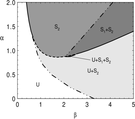
Figure 15: Phase diagram for a Lorentzian distribution of frequencies with width such that $g(0)=1$. Solid and dashed lines show analytical results of the linear stability of the unsynchronized state. Numerics show the bifurcations are supercritical along the solid portions and subcritical along the dashed portion. Dash-dotted lines are saddle-node bifurcations observed in numerical simulations. States are: $U$ - unsynchronized; $S_{1},S_{2}$ synchronized with small and large amplitude respectively.

The phase diagram for the (narrow) Lorentzian distribution with $g(0)=1$ is shown in Fig. 15. The solid and dashed lines are the analytically obtained stability boundaries of the unsynchronized solution. The numerical simulations show that over the dashed portion of the linear instability curve the bifurcation is subcritical, giving a jump in the order parameter magnitude $R$ at onset. In addition the sweeps yield a number of saddle-node bifurcations identified as discontinuous jumps in $R$; these are denoted by dash-dotted lines in Fig. 15; we do not have closed form relations for these boundaries. Thus along the dashed or dash-dotted portions of the boundaries, discontinuous jumps in $R$ occur, either between the unsynchronized state and a synchronized state, or between two synchronized states with different values of $R$. The two synchronized states are labelled $S_{1}$ and $S_{2}$ in Fig. 15. When they coexist at the same $\alpha$ and $\beta$ the state $S_{2}$ has the larger value of $R$, but for both states $R$ may go to zero, connecting continuously with the unsynchronized state $U$, for some values of $\alpha,\beta$.

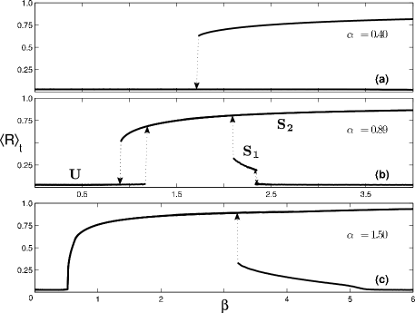
Figure 16: Slices of the phase diagram Fig. 15 showing the time averaged order parameter magnitude $\langle R\rangle_{t}$ as a function of $\beta$ from numerical simulations of the cutoff Lorentzian distribution with $g(0)=1$. In panel (a) the only solutions are the unsynchronized ($U$) and large $R$ synchronized ($S_{2}$) states, while in panels (b) and (c) the small $R$ synchronized solution is also stable. Arrows denote discontinuous jumps that were observed as simulations followed the various solution branches.

Representative phase diagram slices for the Lorentzian case with $g(0)=1$, showing the time-averaged order parameter magnitudes $\langle R\rangle_{t}$ as a function of $\beta$ at fixed $\alpha$, are presented in Fig. 16. In agreement with Eq. (86) the unsynchronized state is stable for all $\beta$ provided $\alpha<0.872$. Simulations find the $S_{2}$ solution is bistable with $U$ over this $\alpha$ range at larger $\beta$ values, as shown in Fig. 16(a). For $\alpha>\alpha_{min}$ the unsynchronized state is unstable over a range in $\beta$. As shown in Fig. 16(b) for a range of $\alpha$ near $\alpha_{\min}$ a subcritical bifurcation occurs at $\beta_{c-}$ as the $U$ solution becomes unstable and $S_{2}$ forms. With increasing $\beta$ $S_{2}$ is the only stable solution until a region of bistability where both synchronized solutions coexist. As shown in the phase diagram there is a small region (labelled $U+S_{1}+S_{2}$) over which all three solutions are simultaneously stable. This region of tristability can be observed in Fig. 16(b), over the $\beta$ range of hysteric transition between $S_{1}$ and $U$ near $\beta=2.3$. With increasing $\alpha$ the system passes through a tricritical point where the subcritical bifurcation at $\beta_{c-}$ becomes supercritical. The tricritical point has a codimension of 2. An example slice at $\alpha$ sufficiently large that the bifurcation is supercritical is shown in Fig. 16(c), where with increasing $\beta$ regions of bistability between the synchronized solutions and then $U$ and $S_{2}$ are observed.

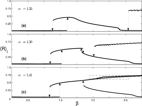
Figure 17: Constant $\alpha$ slices from numerical simulations of the cutoff wide Lorentzian with $g(0)=1/2$. Shown is the time averaged order parameter magnitude $\langle R\rangle_{t}$ for a range of $\beta$ at three $\alpha$ values: (a) $\alpha=1.33$, (b) $\alpha=1.39$, and (c) $\alpha=1.41$. These solutions are observed in an array of $N=1000$ oscillators with a Lorentzian frequency distribution with $g(0)=1/2$ and a cutoff frequency of $\omega_{c}=16$. The dashed box region in panel (c) is examined more closely in Fig. 18.

We now consider a Lorentzian frequency distribution of approximately twice the width. Specifically, we take $g(0)=1/2$ in Eq. (17) or Eq. (80). There are a number of changes to the details of the phase diagram that we do not discuss in detail. Several of these are straightforward consequences of the wider frequency spread: for example the instability of the unsynchronized solution moves to larger $\alpha$ and $\beta$. Instead we focus on two particular features.

The first new feature that is evident from the fixed $\alpha$ cuts shown in Fig. 17 is the reconnection of the branches of synchronized solutions that occurs as $\alpha$ is decreased. In Fig. 17(c), typical of larger values of $\alpha$, the synchronized state growing from the $\beta_{c+}$ instability ends at a saddle-node bifurcation, with the order parameter jumping to larger values as $\beta$ is decreased. This is the same as the behavior for the narrower distribution, Fig. 16. On the other hand for smaller values of $\alpha$, as in Fig. 17(a), this state merges continuously with the larger magnitude state. This change in the topology of the solution branches as $\alpha$ increases occurs through the development of two additional saddle-nodes, as shown in Fig. 17(b) near $\beta=2.1$, and the collision of one of these with the saddle-node terminating the large-$\beta$ upper branch.

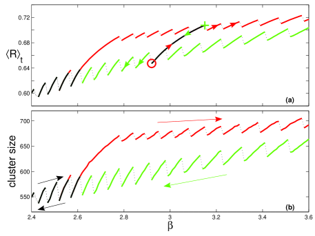
Figure 18: Hysteretic behavior between two boundaries of the large magnitude $\langle R\rangle_{t}$ synchronized solution for a Lorentzian frequency distribution (color online). Shown are the results for $N=1000$, $\alpha=1.41$, and a cutoff Lorentzian distribution with $g(0)=1/2$ and $\omega_{c}=16$. The arrows denote the direction of the $\beta$ sweep, and the states are colored red for an upward sweep, green for a downward sweep, and black if both directions lead to the same state. The + symbols denote the starting point for particular sweeps to traverse a state interior to the band (green for the start of a downward sweep, red for an upward sweep). Panel (a) is a magnification of the dashed box in Fig. 17(c) showing the $\langle R\rangle_{t}$ over a range of $\beta$. In (b) the corresponding size of the synchronized cluster measured by the synchronization index is shown.

Another apparent difference with the wider frequency distribution is the steps displayed by the large amplitude synchronized state at larger $\beta$ in Fig. 17. While these steps also occur with the narrow frequency distribution, their increased amplitude with the wider frequency distribution facilitates the presentation of the behavior. As an example, the dashed region in Fig. 17(c) is shown enlarged in Fig. 18. Panel (a) in this figure plots the time averaged order parameter magnitude $\langle R\rangle_{t}$, while (b) shows that the solution changes correlate exactly with changes in the number of oscillators locked to the synchronized cluster.

Interestingly, the solution follows different trajectories depending on the history of changing $\beta$. For example, if $\beta$ is monotonically increased the system settles onto the upper trajectory of solution steps (colored red) while the lower trajectory of solution steps (colored green) is observed when $\beta$ is monotonically decreased. These solutions overlap at smaller $\beta$ (colored black).

The two solution trajectories are in fact the boundaries of a band of multistable solution branches. This structure is demonstrated in Fig. 18(a) by beginning the system on each of these two boundaries and reversing the direction of $\beta$ variation. Now as $\beta$ changes the solution moves off its boundary along a continuous line to the other boundary where it follows the expected path for that sense of $\beta$ changes. Starting solutions are represented by the + symbols colored for the direction that $\beta$ is to be varied. Beginning on the lower boundary, that is observed when decreasing $\beta$, and increasing $\beta$ from the lower (red) + the oscillators follow the solid (black) line in the direction of the upward arrow to the upper boundary. Likewise, beginning on the upper boundary, that is observed when increasing $\beta$, and decreasing $\beta$ the oscillators display a series of states beginning with the upper (green) + and follow the solid (black) line to the lower boundary in the direction of the downward arrow. In this way, the synchronized solution with large time-averaged order parameter magnitude turns out to be a band of solutions, with striations that can be accessed by appropriate changes in $\beta$. The same is true for the narrow Lorentzian, however the band is smaller.

The steps in the magnitude of the order parameter are found to be associated with jumps in the number of oscillators locked to the phase of the order parameter. Defining a synchronized cluster as the oscillators locked to $\Theta$ we find the discrete steps in $R$ are due to a small group of oscillators leaving the cluster, and then recombining with the cluster one at a time as $\beta$ increases. In Fig. 18(b) the cluster size is measured by the phase synchronization index, defined by Eq. 15, as the number of oscillators with $\chi_{n}=1-\epsilon$, where $\epsilon$ is some small number, $\epsilon<<1$, to allow for some phase variation over the finite time of measurement. With increasing system size any small group of oscillators leaving the cluster can be expected to have decreasing influence on the order parameter.

As the number of oscillators tends to infinity the solution band becomes a region densely populated by these striations as the discrete steps become closer and decrease in length. For the simulations in Fig. 18 $N=1000$ oscillators were used. To investigate finite size effects we also studied this solution using $N=5000$ and $N=10,000$. With increasing system size the individual steps on each solution boundary occur over a more narrow range in $\beta$, becoming shorter in length, and correspondingly more densely packed. Thereby, while the discrete steps will disappear in the infinite size limit the width of the band of synchronized solutions remains nearly the same. In this limit synchronized states will move along one of the striations to the band boundary appropriate for the direction of the $\beta$ sweep.

VII.2 Top-hat Distribution

For bounded distributions we can calculate the linear stability boundaries of both the unsynchronized and the fully synchronized states. We first do this for a uniform bounded distribution, which we call a top-hat distribution.

A top hat distribution centered on $\omega=0$ is given by

$$g(\omega)=\left\{\begin{tabular}[c]{cc}$w^{-1}$&for $\left|\omega\right|\leq w/2$\\ $0$&for $\left|\omega\right|>w/2$\end{tabular}\ \ \ \ \right.$$ (88)

The integrals Eqs. (42) for this distribution are

$$I_{1} =\frac{1}{2w}\tan^{-1}\left[\frac{w/2}{(1+\delta^{2}/4)-w^{2}/16}\right],$$ (89a)

$$I_{2} =\frac{1}{w}\ln\left|\frac{w-2\delta}{w+2\delta}\right|,$$ (89b)

$$I_{3} =\frac{1}{2w}\ln\left[\frac{1+(w-2\delta)^{2}/16}{1+(w+2\delta)^{2}/16}\right],$$ (89c)

$$I_{4} =\left\{\begin{tabular}[c]{cc}$\frac{\pi}{w}$&for$~{}\delta<w/2$\\ $0$&for $\delta>w/2$\end{tabular}\ \ \ \right..$$ (89f)

The self consistency equations (43) and (44) can be solved numerically. The equations simplify in the limit of small $$w$$, and the results here can be displayed in closed form.

In small $w$ limit there is one solution of Eq. (43) giving a locked frequency within the band of (shifted) oscillator frequencies, $\delta<w/2$, for which $I_{1}$ and $I_{3}$ may be neglected in the small $w$ limit. Equation (43) then gives the explicit expression for the frequency offset from mid band

$$\delta\simeq\frac{w}{2}\tanh\left(\frac{\pi}{2\alpha}\right),$$ (90)

and Eq. (44) gives the condition of the parameters at the onset of synchronization

$$(\alpha+\alpha^{-1})\beta_{c}\simeq\frac{2w}{\pi}.$$ (91)

Notice that for large $\alpha$ the locking frequency is close to the center of the band, and the critical condition reduces to

$$\alpha\beta_{c}=2w/\pi,$$ (92)

the value expected from the mapping onto the Kuramoto model for large $\alpha$. For small $\alpha$ on the other hand $\delta$ approaches $w/2$ giving us the result that the locking frequency approaches the upper edge of the band. In this case the onset occurs at $\beta_{c}\simeq 2w\alpha/\pi$. Even for moderate values of $\alpha$ such as $\alpha=1$, the locking frequency is far off the band center (a fraction $0.92$ of the half band width for $\alpha=1$).

The second solution to Eq. (43) in the small $w$ limit gives an order parameter frequency outside of the band, $\delta>w/2$. For small $w$ the frequency is given by

$$\delta\simeq\frac{w}{2}\coth\left(\frac{w}{4\alpha}\right),$$ (93)

and the onset of synchronization occurs at

$$\beta_{c}\simeq 4\alpha.$$ (94)

The solution that grows from this instability is a remarkable state in that it is synchronized in the sense that there is a nonzero value of the order parameter $\left|\psi\right|\neq 0$, but there are no oscillators frequency locked to one another or to the frequency of the order parameter: a plot of the actual frequency distribution as in Figs. 4(a) and 6(a) shows a smooth curve with no plateau. Numerical investigation of this state shows that instead, the distribution of oscillators $\rho(\omega,\theta)$ is enhanced for phases near the phase of the order parameter: oscillators slow down in this vicinity (i.e. $d\bar{\theta}/dt$ becomes smaller), but do not come to rest relative to the order parameter. Now the ordered oscillator frequency plot is continuous, with no plateau of locked oscillators.

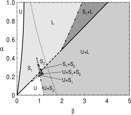
Figure 19: Phase diagram for a top-hat distribution of frequencies of width $w=1$ such that $g(0)=1$. The solid and dashed lines are from the linear stability analysis of the unsynchronized state: the unsynchronized state is unstable for $\beta$ values between the two portions of these lines. The numerical results show that the solid portion is supercritical, whereas the dashed portion is subcritical. Dash-dotted lines are saddle-node bifurcations from numerical simulations. The dotted line is the stability boundary of the fully locked solution calculated using the methods of Sec. VI. States are as in Fig. 15 with, in addition, $L$ denoting the fully locked state.

The linear instability boundaries for a top-hat distribution of full width $w=1$ (giving $g(0)=1$) are shown as the solid and dashed lines in Fig. 19. The approximate solutions Eqs. (90-94) turn out to be quite accurate even for $w=1$: the approximate curves are indistinguishable from the numerical curves in Fig. 19. Note that unlike the case of the Lorentzian distribution, the linear instability persists for $\alpha,\beta\rightarrow 0$. In this limit the frequency of the order parameter is right at the edge of the distribution of oscillator frequencies. The discontinuity of the distribution of oscillator frequencies at the band edge seems to be responsible for the persistence of the instability to small values of the coupling constants.

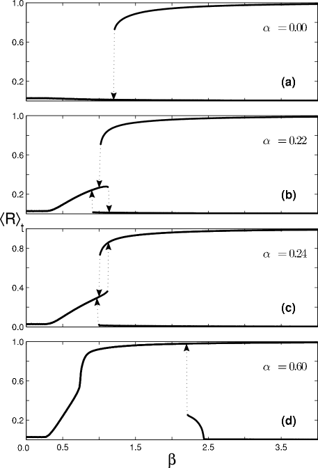
Figure 20: Phase diagram slices observed in simulations with a top-hat frequency distribution. The time averaged order parameter magnitude $\langle R\rangle_{t}$ over a range of $\beta$ is shown for constant $\alpha$: (a) $\alpha=0$, (b) $\alpha=0.22$, (c) $\alpha=0.24$, and (d) $\alpha=0.60$. In these simulations $N=1000$ and the width $w=1$.

The boundary of the fully-locked solution calculated using the analysis of Sec. VI is also shown on Fig. 19 as the dotted line. In addition we have performed a careful numerical scan of the $\alpha-\beta$ plane for $N=1000$ or $10000$ oscillators with a uniform distribution of full width unity. These results confirm the analytic predictions, and again show additional transitions that are inaccessible to our analytic calculations. The numerics shows that the linear instability from the unsynchronized state is subcritical over the dashed portion of the linear instability curves as shown in the figure. Other saddle-node bifurcations are shown as dash-dotted lines. The complete phase diagram is quite complicated. Some representative numerical sweeps are shown in Fig. 20.

VII.3 Triangular Distribution

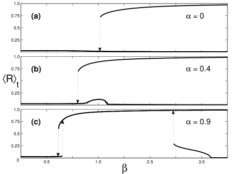
Figure 21: Solutions observed in simulations of $N=1000$ oscillators having a triangular frequency distribution with $g(0)=1$. The time-averaged order parameter magnitude $\langle R\rangle_{t}$ is plotted over a range of $\beta$ at fixed $\alpha$: (a) $\alpha=0.0$, (b) $\alpha=0.4$, and (c) $\alpha=0.9$.

We finally present results for when the oscillators have a triangular frequency distribution

$$g(\omega)=\left\{\begin{tabular}[c]{cc}$(4/w^{2})(w/2-\left|\omega\right|)$&for $\left|\omega\right|\leq w/2$\\ $0$&for $\left|\omega\right|>w/2$\end{tabular}\ \ \ \ \ \ .\ \right.$$ (95)

This is the case studied in reference CZLR04 . The triangular distribution is bounded, and so can have a fully locked state as for the top-hat distribution, but does not have the discontinuity in $g(\omega)$ at the edge of the distribution leading to singular behavior as $\alpha,\beta\rightarrow 0$ for that distribution. The results are compiled from the linear stability analysis of the unsynchronized and fully locked state, as well as numerical investigation, usually of $1000$ oscillators, as shown in Fig. 21. The integrals Eqs. (42) needed for the stability analysis of the unsynchronized state can again be done in closed form, but the results are too cumbersome to list here.

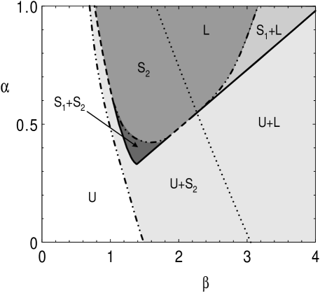
Figure 22: Phase diagram for a triangular distribution of frequencies of full width $w=2$ such that $g(0)=1$. Symbols and lines are as in Fig. 19.

The results for $\beta_{c}(\alpha)$ for $g(0)=1$ (a width $w=2$) given by numerically solving Eqs. (43) and (44) are shown as the full and dashed lines in Fig. 22. Simulations show that this transition is subcritical over the dashed portions. In addition, as in Fig. 19, saddle-node bifurcations identified by jumps in the order parameter magnitude $R$ in the simulations are shown by dash-dotted curves.

As for the top-hat distribution, the large $\beta$ limit of the instability region corresponds to an order parameter frequency outside of the band of shifted oscillator frequencies, so that there is no oscillator with a frequency equal to that of the order parameter. This seems to be the typical result for a bounded distribution. For the unbounded Lorentzian distribution on the other hand, there are some oscillators that lock to the order parameter frequency at the large $\beta$ instability. However even for this distribution, for most values of $\alpha$ the order parameter frequency is far in the tails of the distribution, and there are few oscillators at this frequency. Presumably the effect of these locked oscillators on the critical $\beta$ is small, so that the dominant physics at this transition for bounded and unbounded distributions is not very different. Near the smallest $\alpha$ where the upper and lower stability boundaries meet, the order parameter frequencies of the two solutions approach the edge of the band (from either side).

VIII Conclusions

In summary, we have analyzed in detail a model for the synchronization of nonlinear oscillators where the ordering arises from the reactive coupling between the oscillators, combined with the nonlinear frequency pulling of the individual oscillators. Such a model may be a more realistic description than previous models for a variety of physical systems where dissipation plays a relatively minor role, for example high-Q mechanical oscillators and some optical systems. More generally, the model may give a more complete description of synchronization where the individual frequencies are internally tuned in response to a mismatch with other frequencies in the ensemble, such as might occur in biological systems.

We have presented detailed analytic calculations for the onset of partial synchronization from the unsynchronized state, as well as the existence and bounds of the fully locked synchronized state at large coupling and nonlinearity for the cases of bounded frequency distributions. The analytical calculations together with numerical simulations have been used to construct detailed phase diagrams of the different synchronized states as a function of the two parameters of the model, the coefficient of the nonlinear frequency pulling $\alpha$ and the coupling constant $\beta$, for various frequency distributions. The intersections of the various synchronized states lead to rich phase diagrams.

There are a number of interesting features of these phase diagrams. The instability of the unsynchronized state occurs over a limited range of $\beta$ at fixed $\alpha$, so that the unsynchronized state regains stability at very large values of the coupling strength, although a large amplitude synchronized state also occurs here, often terminated by a saddle-node bifurcation as $\beta$ is decreased. This large amplitude synchronized state may also survive down to $\alpha=0$, i.e. even in the absence of the nonlinear frequency pulling. For bounded distributions the state that develops from the linear instability of the unsynchronized state as $\beta$ is decreased is synchronized (the order parameter is nonzero) but there is no frequency locking. The phase diagrams also show a wide variety of multistability, with one or more synchronized states and the unsynchronized state coexisting over various parameter ranges, leading to hysteresis as the parameters are varied. The multistability may be particularly dramatic for the large amplitude synchronized states such as displayed in Fig. 18 where many synchronized states coexist, leading to a band of solutions in the large $N$ limit.

- (1) M. Bennett, M. F. Schatz, H. Rockwood, and K. Wiesenfeld, Proc. Roy. Soc. Series A 458, (2002)
- (2) E. Buks and M. L. Roukes, J. Microelectromech. Sys. 11, 802 (2002)
- (3) M. Sato, B. E. Hubbard, A. J. Sievers, B. Ilic, D. A. Czaplewski, and H. G. Craighead, Phys. Rev. Lett. 90, 044102 (2003)
- (4) P. C. Matthews, R. E. Mirollo, and S. H. Strogatz, Physica D 52, 293 (1991)
- (5) A. T. Winfree, J. Theor. Bio. 16, 15 (1967)
- (6) Y. Kuramoto, in “International Symposium on Mathematical Problems in Theoretical Physics”, ed. H. Arakai, Lecture Notes in Physics, 39, 420 (Springer, New York, 1975)
- (7) J. A. Acebron, L. L. Bonilla, C. J. P. Vicente, F. Ritort, and R. Spigler, Rev. Mod. Phys. 77, 137-184, (2005)
- (8) H. Sakaguchi, Prog. Theor. Phys, 79, 39 (1988)
- (9) M. C. Cross, A. Zumdieck, R. Lifshitz, and J. L. Rogers, Phys. Rev. Lett. 93, 224101 (2004)
- (10) M. Zalalutdinov, A. Zehnder, A. Olkhovets, S. Turner, L. Sekaric, B. Ilic, D. Czaplewski, J. M. Parpia, and H. G. Craighead, Appl. Phys. Lett. 79, 695 (2001)
- (11) B. Ilic, S. Krylov, K. Aubin, R. Reichenbach, and H. G. Craighead, Appl. Phys. Lett. 86, 193114 (2005)
- (12) D. G. Aronson, G. B. Ermentrout, and N. Kopell, Physica D 41, 403 (1990)
- (13) R. Lifshitz and M. C. Cross, Phys. Rev. B67, 134302 (2003)