Quantum spectrum as a time series : Fluctuation measures

Abstract

The fluctuations in the quantum spectrum could be treated like a time series. In this framework, we explore the statistical self-similarity in the quantum spectrum using the detrended fluctuation analysis (DFA) and random matrix theory (RMT). We calculate the Hausdorff measure for the spectra of atoms and Gaussian ensembles and study their self-affine properties. We show that DFA is equivalent to $\Delta_{3}$ statistics of RMT, unifying two different approaches. We exploit this connection to obtain theoretical estimates for the Hausdorff measure.

The fluctuations in physical systems carry important information about the system. In the context of quantum systems, the spectral fluctuations reveal whether the corresponding classical dynamics is regular or chaotic or a mixture of both boh1 . It is well known that for the classically regular systems, the quantum eigenvalues are uncorrelated while for the chaotic systems, the eigenvalues tend to display a certain degree of correlation, which is dictated by the symmetry properties of the system such as the presence or absence of rotational and time reversal invariance. Typically, the spectrum of high dimensional quantum systems like the atoms, molecules and nuclei belong to the latter class. This equivalence between the nature of classical dynamics and spectral fluctuations in the corresponding quantized system is generally through an analogy with random matrix ensembles boh1 and has been verified in many simulations and experiments rmt .

Recently a different approach has been suggested. It is possible to consider suitably transformed eigenvalues of a quantum system as a time series. Then, using time series analysis methods, it was shown that the quantum systems display $f^{-\gamma}$ noise where $1\leq\gamma\leq 2$ depends on the classical dynamics in the system rel . In particular, for the chaotic systems the level fluctuations display $1/f$ noise. So do the levels of complex nuclei rel . In contrast, for the regular systems we get $1/f^{2}$ noise. Hence, the spectral fluctuations can be characterized without reference to random matrix models.

This is reminiscent of following types of time series. In the Brownian motion or random walk time series $x_{t},t=1,2,\dots,N$, the successive increments of the series are uncorrelated. The variance of this process is $\mbox{var}(x)\propto t^{2H},(H=1/2)$, where $H$ is the Hausdorff measure. In this case, the power spectrum gives rise to $1/f^{2}$ noise tur . Thus, regular classical systems with uncorrelated quantum levels are analogous to a series of Brownian motion path. On the other hand, one could also imagine a time series with $1/f$ noise. There are many mechanisms and processes that produce $1/f$ noise obf . In a chaotic system, the eigenvalues of the corresponding quantum system contains certain degree of correlation and it displays $1/f$ noise. In this case, $H=0$ and corresponds to variance being time-independent. In general, for $0<H<1,\gamma=2H+1$. In terms of the exponent $H$, our interest is in the regular ($H=1/2$) and chaotic limits ($H=0$) for the fluctuations of the spectral ‘time series’. This region $0<H<1/2$ corresponds to anti-persistent time series, i.e, the one which has opposing trends at successive time steps. Visually an anti-persistent time series presents a very rough profile as compared to $H=1/2$ series. In fact, $H$ is also used to characterize the roughness of surfaces and profiles.

Such an anti-persistent series is also a self-affine fractal and displays statistical self-similarity that scale differently in different directions. Mathematically, it implies, $y(Ht)\approx t^{-H}y(t)$ where the symbol $\approx$ represents statistical equality. Note that the power spectrum is a measure of the strength of frequencies in Fourier space but the fluctuation function and the Hausdorff measure, taken together, indicate the structure of the spectrum at various spectral scales. This structure is related to the classical periodic orbits of the system through semiclassical theories like the Gutzwiller’s trace formula gut . Hence, it is important to understand the self-affine properties of the spectrum since it has implications at the level of classical dynamics of the system.

The idea of characterizing fluctuations and its scaling is of interest in other areas as well. For instance, the surface-height fluctuations in the surface growth processes reflect the morphological changes that determine the physical and chemical processes such as crystal growth, metal deposition etc. ro2 . Fluctuations in the EEG series might tell us about the nature of physiological process taking place eegdfa . In all these cases, fluctuations and how it scales provide an important clue to the physical process under study. Hence, the results presented here have relevance in fields beyond quantum physics.

In this paper, we take the time series point of view for the quantum spectrum and compute the exponent $H$ for levels of Lanthanide atoms (Sm, Pm and Nd) and RMT ensembles using DFA method dfap . Note that the value of $\gamma$ does not necessarily guarantee self-affine nature greis . We show that the DFA of order 1 is related to $\Delta_{3}$ statistics of RMT and exploit it to obtain theoretical fluctuation functions and $H$. We show that the time series of level sequences and a random time series both with the same value of $H$ have the same fluctuation properties.

We denote a spectrum of discrete levels, belonging to either a random matrix or a given atomic system, by $E_{i},i=1,2,\dots,n+1$. Then, its integrated level density, i.e, the total number of levels below a given level, can be decomposed into an average part plus an oscillatory contribution, $N(E)=N_{av}(E)+N_{osc}(E)$. Spectral unfolding is effected by the transform, $\lambda_{i}=N_{av}(E_{i})$, such that the mean level density of the transformed sequence $\{\lambda\}$ is unity. All further analysis is carried out using $\{\lambda\}$. For instance, the level spacing is, $d_{i}=\lambda_{i+1}-\lambda_{i},i=1,2,\dots,n$. Main object of interest in this paper is the fluctuations in the ‘time series’ of levels given by,

$$\delta_{m}=\sum_{i=1}^{m}(d_{i}-\langle d\rangle)\equiv-N_{osc}(E_{m+1});\;m=1,\dots,n.$$ (1)

Note that $\delta_{m}$ is formally analogous to a time series with the time index denoted by $m$ rel . The power spectrum $S(f)$ of $\delta_{m}$ displays a power law, i.e, $S(f)\sim f^{-\gamma}$, where $1\leq\gamma\leq 2$ rel . In particular, if the system is regular, $\gamma=2$ and for Gaussian ensembles and the chaotic systems, $\gamma=1$. Thus, $1/f$ noise should correspond to $H=0$. A $H=0$ random time series should have a profile similar to levels of Gaussian ensembles and atoms as seen in Fig. 1(a-c).

To obtain $\delta_{m}$, we needed to unfold the spectrum. This puts the spectra from various systems on the same footing amenable to direct comparison. For the atomic systems, unfolding was done using an empirical function to fit the given levels. For the Gaussian ensembles the Wigner’s semi-circle law rmt was used for unfolding.

First, we show the results from Lanthanide atoms. The atoms in this series exhibit complex configuration mixing and spectra. Recently, a series of studies on the statistical properties of these levels from RMT point of view were reported dk . All the calculations for levels of Sm, Nd, Pm were done using the grasp92 code and for details we refer to grasp . In Fig. 1(a), we show $\delta_{m}$ for levels obtained from Sm. Note that the profile is similar to levels from Gaussian Orthogonal Ensemble (GOE), shown in Fig. 1(b), and a random time series with $H=0$ ( Fig. 1(c) ). This is in contrast to the level profile of Gaussian Diagonal Ensemble (GDE) ( Fig. 1(d)) defined as an ensemble of diagonal matrices whose elements are Gaussian distributed random numbers.

To quantitatively obtain the exponent $H$, we compute it using the detrended fluctuation analysis (DFA) technique, which has become a popular tool to study long range correlations in time series dfap . DFA is based on the idea that if the time series contains nonstationarities, then the variance of the fluctuations can be studied by successively detrending using linear, quadratic, cubic … higher order polynomials in a piecewise manner. The entire time series is divided into segments of length $s$ and in each of them detrending is applied and variance $F^{2}(s)$ about the trend is computed and averaged over all the segments. This exercise is repeated for various values of $s$. For a self-affine fractal, we have,

$$F(s)\propto s^{H}$$ (2)

where $0<H<1$. In Table 1, we show the numerical estimates of $H$ obtained for various atomic and Gaussian ensemble cases. The results tabulated alongside represent average of $F(s)$ taken over an appropriate ensemble. For instance, for the Sm levels, the ensemble consists of 6 sequences each with 650 levels. Similarly for Pm and Nd. In the case of Gaussian ensembles of RMT, the results were obtained from ensemble of 50 level sequences each with 4600, 3900, 2100 levels respectively for Gaussian Orthogonal ensemble, Unitary ensemble (GUE) and Symplectic ensemble (GSE). For the uncorrelated levels from GDE, we get $H=0.508$ in good agreement with the expected value of 1/2. For the atomic and Gaussian ensembles, the value of $H$ is close to zero. In such cases standard DFA becomes inaccurate and DFA is performed after integrating $\delta_{m}$ once more so that the new exponent is $H_{1}=H+1$. Table 1 shows that $H_{1}$ is close to unity for atomic and Gaussian ensembles. Thus, the GDE levels are self-affine fractal with $H=1/2$ but those of atomic and Gaussian ensembles $(H=0)$ do not fall in this class.

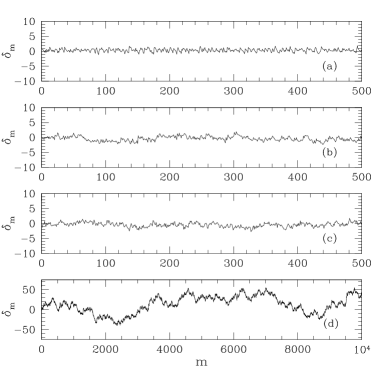
Figure 1: $\delta_{m}-m$ curve for (a) Sm I atomic levels (b) GOE levels (c) time series with $H=0$ and (d) GDE levels. Note that (a,b,c) have qualitatively similar features as opposed GDE levels in (d).

Table 1: Numerical estimates of $H_{1}$ and $H$.

System	Hausdorff measure ($H$)	$H_{1}$
Sm	0.045	1.045 $\pm$ 0.031
Pm	-0.025	0.975 $\pm$ 0.024
Nd	-0.003	0.997 $\pm$ 0.013
GOE	0.0003	1.0003 $\pm$ 0.0083
GUE	0.0047	1.0047 $\pm$ 0.0089
GSE	0.0025	1.0025 $\pm$ 0.0125
GDE	0.5080	1.5080 $\pm$ 0.0044

In order to obtain analytical estimate for the value of $H$, we appeal to the $\Delta_{3}(s)$ statistic widely studied in RMT to quantify rigidity of spectrum, i.e, given a level, a rigid spectrum will not allow any flexibility in the placement of the next level. $\Delta_{3}(s)$ is a measure of this flexibility or conversely the rigidity. It is defined by,

$$\Delta_{3}(\bar{\lambda},s)=\frac{1}{2s}\min_{a,b}\int^{\bar{\lambda}+s}_{\bar{\lambda}-s}[n(\lambda)-a\lambda-b]^{2}d\lambda$$ (3)

where $n(\lambda)=n_{av}(\lambda)+n_{osc}(\lambda)$ is the integrated level density for the unfolded spectrum $\{\lambda\}$ and $a$ and $b$ are the parameters from linear regression and $\bar{\lambda}$ is any reference level. Now, $\Delta_{3}(s)$ is an average over various choices of $\bar{\lambda}$. Notice that $n(\lambda)=N(E)$ and due to unfolding procedure, $n_{av}(\lambda)=\lambda$. This implies that, $n_{osc}(\lambda)=N_{osc}(E)$. Then, we could rewrite Eq. (3) as,

$$\Delta_{3}(\bar{\lambda},s)=\frac{1}{2s}\min_{a,b}\int^{\bar{\lambda}+s}_{\bar{\lambda}-s}[n_{osc}(\lambda)-(a-1)\lambda-b]^{2}d\lambda$$ (4)

Now we discretize this equation to relate $\Delta_{3}(s)$ with the standard fluctuation function $F(s)$ obtained by DFA. Substituting from Eq. (1) for $n_{osc}(\lambda)$, we get,

$$\begin{split}\Delta_{3}(s)=&\frac{1}{M}\sum_{j=0}^{M}\frac{1}{2s}\sum_{m=j+1}^{j+2s}[\delta_{m}-Y(\lambda_{m})]^{2}\\ =&\frac{1}{M}\sum_{j=0}^{M}F^{2}(s,j)=F^{2}(s)\end{split}$$ (5)

where $Y(\lambda_{m})=(a^{*}-1)\lambda_{m}+b^{*}$ with best fit parameters $a^{*}$ and $b^{*}$ and $j$ indexes $M$ different choices of $\bar{\lambda}$. Since the DFA is applied with linear detrending on segments of length $s$, then Eq. (5) boils down to $\Delta_{3}(s)=F_{1}^{2}(s)$, and the subscript denotes DFA(1). Then, ensemble averaging and writing $F_{1}(s)$ in terms of $\Delta_{3}(s)$, we have,

$$\langle F_{1}(s)\rangle=\langle\Delta_{3}(s)^{1/2}\rangle$$ (6)

This main result of the paper shows DFA(1) to be equivalent to $\Delta_{3}$ statistic. From RMT, the averages for $\langle\Delta_{3}(s)\rangle$ are well known. For the GDE, we have $\langle\Delta_{3}^{\mbox{GDE}}(s)\rangle=s/15$. Then, the result for uncorrelated set of levels is,

$$\langle F_{1}(s)\rangle\sim s^{H}\sim\left(\frac{s}{15}\right)^{1/2}$$ (7)

On a log-log plot we expect a slope of $H=1/2$. This is amply verified in Fig. 2(d) for GDE with slope 0.508. In our numerical simulation, GDE consists of 50 level sequences of 15000 levels each.

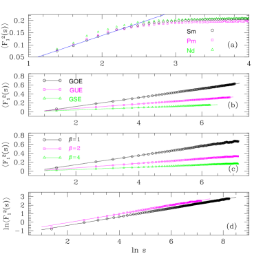
Figure 2: (Color online) The fluctuation function $\langle{F_{1}}^{2}(s)\rangle$ in a semi-log plot for (a) atomic levels, (b) Gaussian ensembles and (c) random time series with $H=0$ and power spectrum $1/\beta f$. (d) shows $\ln\langle{F_{1}}^{2}(s)\rangle$ vs $\ln s$ for GDE and a random walk time series. The slopes of best fit (solid) lines are quoted in the text.

The numerical results for atomic levels and Gaussian ensembles in Table 1 show that $H\approx 0~{}(H_{1}\approx 1)$. To make correspondence with $H_{1}$, we consider modified $\Delta_{3}$ statistics given by,

$$\Delta(\bar{\lambda},s)=\frac{1}{2s}\min_{a,b}\int^{\bar{\lambda}+s}_{\bar{\lambda}-s}[\lambda~{}n(\lambda)-a\lambda-b]^{2}d\lambda$$ (8)

which corresponds to integrating the $\delta_{m}$ once more before performing DFA on it. We obtain the asymptotic random matrix average to be new ,

$$\langle\Delta(s)\rangle\sim s^{2H_{1}}\propto s^{2}$$ (9)

for all the three ensembles. Then, using Eq 6, $\langle F_{1}(s)\rangle\propto s$ and hence the theoretical slope $H_{1}=1$ and corresponds to standard Hausdorff measure $H=0$. The numerical values in last column of Table 1 confirm this RMT based result. For Pm and Nd, note that the small negative values for $H$ are in the error bar as seen by the error estimates provided.

Using the time series analogy, we explore the nature of fluctuations at $H=0$ for Gaussian ensembles. This, in turn, throws further light on the fluctuation properties of $H=0$ time series. From RMT we have, $\langle\Delta_{3}(s)\rangle_{\beta}\approx\frac{\ln 2\pi s}{\beta\pi^{2}}$, where $\beta=1,2,4$ for GOE, GUE and GSE respectively. Substituting this in Eq. (6), the fluctuation function at $H=0$ is,

$$\langle{F_{1}}(s)\rangle\sim\left(\frac{\ln 2\pi s}{\beta\pi^{2}}\right)^{1/2}$$ (10)

At $H=0$, the ensemble averaged fluctuations display logarithmic scaling with length of level sequence $s$ considered. For convenience, we plot $\langle{F_{1}}^{2}(s)\rangle$ in a semi-log plot. Then we expect slopes for level sequences from GOE, GUE and GSE to be $1/\beta\pi^{2}$. In Fig. 2(a), we show results from atomic levels of Sm, Pm and Nd. In all the three cases, the straight-line obtained shows that the DFA fluctuation function is in good agreement with the theoretical result based on $\Delta_{3}(s)$ statistics. Their slopes, 0.105, 0.104 and 0.109 for Sm, Pm and Nd agree closely with $1/\pi^{2}$. The deviations for $\ln s>2.2$ occurs due to breakdown of universality in the presence of system specific information. This is related to the period of the short periodic orbits in the atomic system berry . Thus, quantum spectrum of complex atoms can be characterized by $H=0$ and display logarithmic scaling. Similar results are obtained for the Gaussian ensembles. Fig. 2(b) shows linear relationship in semi-log plot for levels from GOE, GUE and GSE. The measured best fit slopes 0.0995 $(\beta=1)$, 0.0511 $(\beta=2)$, 0.0257 $(\beta=4)$ closely approximate the theoretical value $1/\beta\pi^{2}$. The DFA applied to spectral levels can distinguish between the three ensembles. This is not possible with the power spectrum method unless one measures the slope and the intercept together. Intercept measurement is often difficult due to deviations from scaling for small frequencies.

What happens to an anti-persistent time series at $H=0$ ? We generate random time series with $H=0$ and power spectrum $S(f)=1/2\beta\pi^{2}f$. The technique is to generate Gaussian random numbers $u$ and take its Fourier transform to obtain $\tilde{u}$. Then, take the inverse Fourier transform of $\tilde{u}\sqrt{|S(f)|}$ to obtain a time series with the required properties rang . By varying $\beta$, we get a synthetic random time series that will mimic level fluctuations of GOE, GUE and GSE. The DFA applied to 10 member ensemble of such time series (each of length 5000) is shown in Fig. 2(c). On a semi-log plot, they produce the expected linearity and slopes 0.1035, 0.0517 and 0.0258 agree quite well with the theoretically expected result $1/\beta\pi^{2}$. We conclude that an appropriate time series with $1/f$ noise is similar to a level spectrum from random matrix ensembles and complex atoms and both display fluctuations that scale in a logarithmic manner at $H=0$. These results, viewed in conjunction with Bohigas et. al. conjecture boh1 , mean that we can expect the spectrum of classically regular systems to be characterized by $H=1/2$ and chaotic systems by $H=0$.

Even though we motivated our work using quantum systems, we emphasize that if the spectrum is viewed as a time series, then we can apply our main results to any classical system where self-affinity of the time series is relevant. For instance, in studies of surface roughness, growth models where surface morphology determines the properties of the physical and chemical processes. Examples of surface growth are the evolution of landscapes, vapor deposition, propagation of flame fronts and growth of bacterial colonies etc. ro2 . In these cases, a relevant quantity of interest is the correlation function for the surface heights $h({\mathbf{x}})$, $C({\mathbf{r}})=\langle|h({\mathbf{x}})-h({\mathbf{x}+r})|^{2}\rangle^{1/2}$. In many cases, $C(r)\sim r^{H}$ over a large range of length scales, i.e, many such growing surfaces are self-affine fractals. In Ref. pal a modified form for the correlation function of rough surfaces is studied which gives logarithmic fluctuations, similar to Eq. (10) obtained above, as $H\to 0$. This has been confirmed by numerical simulations of surfaces as well as from experimental results of thin-film evaporation pal . Another feature of surface growth is the existence of roughening transition for certain critical parameter values. At roughening transition, the exponent is $H=0$ and $C(r)$ displays logarithmic fluctuations as experimentally verified for Ag(115) sample ro1 . We have also shown that $H=0$ corresponds to log fluctuations using random matrix methods. Hence, taking the time series perspective and RMT could be beneficial for various other problems.

To summarize, we treat the quantum spectrum like a time series. In this picture, the uncorrelated spectral levels behave like a random walk series with Hausdorff measure $H=1/2$ and is a self-affine fractal. For the spectrum of complex atoms and Wigner-Dyson random matrix ensembles, $H=0$, an anti-persistent time series. We show that the DFA is equivalent to $\Delta_{3}$ statistics of RMT and we exploit this connection to obtain theoretical estimates for $H$. This shows that at $H=0$ the spectral fluctuations display logarithmic behavior, a feature seen in many experimental and model simulations in surface growth studies. Thus, $H=0$ is an unusual and interesting limit and will require further investigation.

We thank Prof. J. C. Parikh, Dr. P. Panigrahi, Prof. V. B. Sheorey and P. Manimaran for useful discussions.

References

- (1) O. Bohigas et. al., Phys. Rev. Lett. 52, 1 (1984).
- (2) M. L. Mehta, Random Matrices, 2nd ed. (Academic Press, New York, 1991).
- (3) A. Relao et. al., Phys. Rev. Lett. 89, 244102 (2002); S. N. Evangelou et. al., Phys. Lett. A 334, 331 (2005); E. Faleiro et. al., Phys. Rev. Lett. 93, 244101 (2004); M. S. Santhanam and J. N. Bandyopadhyay, Phys. Rev. Lett. 95 114101 (2005).
- (4) D. Turcotte, Chaos and Fractals in Geology and Geophysics, 2nd Ed. (Cambridge University Press, New York, 1997).
- (5) Bruce J. West and M. F. Shlesinger, American Scientist 78, 40 (1990).
- (6) M. C. Gutzwiller, Chaos in Classical and Quantum Mechanics, (Springer, Heidelberg, 1990).
- (7) P. Meakin, Phys. Rep. 235, 189 (1993).
- (8) C-K. Peng et. al., Chaos 5, 82 (1995).
- (9) C-K. Peng et. al., Phys. Rev. E 49, 1685 (1994).
- (10) N. P. Greis and H. S. Greenside, Phys. Rev. A 44 2324 (1991).
- (11) D. Angom and V. K. B. Kota, Phys. Rev. A 67, 052508 (2003); Phys. Rev. A 71, 042504 (2005); D. Angom et. al., Phys. Rev. E 70, 016209 (2004).
- (12) F. A. Parpia et. al., Comp. Phys. Commun. 94, 249 (1996).
- (13) For uncorrelated levels, ; M. S. Santhanam and J. N. Bandyopadhyay (under preparation).
- (14) M. V. Berry, Proc. R. Soc. Lond. A 422, 7 (1989).
- (15) G. Rangarajan and M. Ding, Phys. Rev. E 61, 4991 (2000).
- (16) G. Palasantzas, Phys. Rev. E, 49, 1740 (1994); Phys. Rev. B, 48 14472 (1993).
- (17) M. S. Hoogeman et. al., Phys. Rev. Lett. 82, 1728 (1999); Michael Lassig, Nuclear Phys. B 448 [FS], 559 (1995).