Discrete Embedded Solitons

Abstract

We address the existence and properties of discrete embedded solitons (ESs), that is localized waves existing inside the phonon band in a nonlinear dynamical-lattice model. The model describes a one-dimensional array of optical waveguides with both $\chi^{(2)}$ (second-harmonic generation) and $\chi^{(3)}$ (Kerr) nonlinearities, for which a rich family of ESs are known to occur in the continuum limit. First, a simple motivating problem is considered, in which the $\chi^{(3)}$ nonlinearity acts in a single waveguide. An explicit solution is constructed asymptotically in the large-wavenumber limit. The general problem is then shown to be equivalent to the existence of a homoclinic orbit in a four-dimensional reversible map. From properties of such maps, it is shown that (unlike ordinary gap solitons), discrete ESs have the same codimension as their continuum counterparts. A specific numerical method is developed to compute homoclinic solutions of the map, that are symmetric under a specific reversing transformation. Existence is then studied in the full parameter space of the problem. Numerical results agree with the asymptotic results in the appropriate limit and suggest that the discrete ESs may be semi-stable as in the continuous case.

I Introduction

An embedded soliton (ES) is an isolated solitary wave in a non-integrable system that resides insides the continuous spectrum of linear waves. Unlike regular gap solitons, the existence of ESs in continuum models is generally of codimension-one in the model’s parameter space. That is, they are embedded into wider families of generalized solitary waves which have nonvanishing periodic tails attached to them, such that the ES occurs at isolated values of the frequency, or other intrinsic parameter of the solution family at which the tail’s amplitude vanishes. The concept of ESs was introduced in YaMaKa:99 (see also ChMaYaKa:01 ; YaMaKaCh:01 for more details), although particular examples of waves of this kind were actually known earlier (but not under this name) ChGr:97 ; FuEs:97 ; ChMaFr:98 . In the last few years, ESs have been shown to be of relevance in a diverse range of nonlinear-wave models, see, e.g.,  KoChBuSa:02 ; AtMa:01 ; EsFuGo:03 ; Ya:03 and references therein. One of their characteristic properties is that they are typically, at best, semi-stable. That is, the linearization around them gives rise to no unstable eigenvalues, but a non-trivial zero-eigenvalue mode can be found. The latter leads to an algebraic-in-time instability for energy-decreasing perturbations, and a similar algebraic-in-time relaxation back to the original pulse for energy-increasing perturbations PeYa:02 . Only in special cases of systems which have more than one dynamical invariant, or for which the travelling-wave system is reversible but not Hamiltonian, have examples been found of ESs that are truly asymptotically stable Ya:03 . Also known are physically relevant models with special symmetries that support continuous (rather than discrete) families of ESs, and a large part thereof may be stable Mak ; Merhasin .

All the above-cited examples pertain to continuum models. A fundamental issue is whether solitons of the embedded type may also occur in discrete nonlinear equations modelling dynamical lattices. For example, in ChKi:99 it was argued that moving topological defects in Frenkel-Kontorova (discrete sine-Gordon) lattices can meaningfully be described as embedded kinks. Some of specific examples of moving discrete solitons constructed by means of the inverse method (a model is sought for to which a given moving soliton is an exact solution Flach ) may also have the embedded character. Such waves, which connect a zero state to itself, translated through a multiple of the period of the lattice potential (the ‘topological charge’), were first (indirectly) identified by Peyrard and Kruskal PeKr:84 and have later received much attention in a wide variety of applications KiBr:98 . In a co-moving frame, these waves should be thought of as localized solutions to infinite-dimensional advance and delay (nonlocal) equations, see works SaZoEi:00 ; AiChRo:03 where branches of embedded kinks with the topological charge 1 and 2 were computed. Another recent study ESdiscrete reported the existence of ESs in a discrete lattice of the Ablowitz-Ladik type, but with a quintic nonlinearity added to the usual cubic terms, and also with an additional next-nearest-neighbor linear coupling. By tuning the nonlinear terms, an explicit analytical solution for a discrete ES was found in that model (which somehow resembles the above-mentioned inverse method). Apart from these, we are aware of no other work that systematically considers the issue of ESs in discrete models.

A general objective of this paper is to understand the existence and multiplicity properties of discrete solitons in lattice systems for which the corresponding continuum model is known to support ESs. The first fundamental issue is whether the codimension of their existence is preserved under discretization. In dissipative systems, solitary pulses are supported due to the balance between forcing and damping, hence the corresponding homoclinic orbits are always of codimension one. Thus, formally similar to ESs, dissipative solitons typically exist as solutions to the corresponding stationary ordinary differential equation at discrete values of a relevant parameter (temporal or spatial frequency, depending on the physical realization). Then, it will generically happen that, under the discretization of that equation, the codimension of the solitons decreases. This is possible because discretization of homoclinic orbits to hyperbolic equilibria leads to transverse homoclinic connections that exist for a range of parameter values FiSc . However, for ESs we shall show that, in contrast, discrete ESs typically keep the same codimension as their continuum counterparts, i.e., they also exist at discrete values of the corresponding physical parameter.

In this work, we restrict ourselves to a discretization of a single continuum model, for which the discrete counterpart finds a direct physical interpretation. In fact, our results and methodology will carry over to other discretized models that support ESs (this expectation is supported by the general fact that equations of the discrete nonlinear-Schrödinger type, that we consider below, may be derived as an asymptotic limit from a much larger class of discrete models Morgante ). Specifically, we shall start with the continuum model in which ESs were identified YaMaKa:99 . It describes an optical medium with competing quadratic ($\chi^{(2)}$) and cubic ($\chi^{(3)}$) nonlinearities (see Bang1 ; Bang2 ; Bang3 and references therein for physical applications). In this model, the evolution variable $z$ is the propagation distance in the nonlinear optical waveguide, and the variable $t$ is either the reduced time (in the case of temporal solitons) or, which is more physically relevant, a transverse spatial coordinate in a planar waveguide. In the temporal case, such a model can be written in dimensionless form as (see detailed explanations in reviews Review ; DiscrChi2soliton )

$$i\frac{\partial u}{\partial z}+\frac{1}{2}\frac{\partial^{2}u}{\partial t^{2}}+u^{\ast}v+\gamma_{1}(|u|^{2}+2|v|^{2})u=0,$$

(1)

$$i\frac{\partial v}{\partial z}+\frac{\delta}{2}\frac{\partial^{2}v}{\partial t^{2}}+qv+\frac{1}{2}u^{2}+2\gamma_{2}(|v|^{2}+2|u|^{2})v=0,$$

where $u$ and $v$ are the local amplitudes of the fundamental-frequency (FF) and second-harmonic (SH) fields, an asterisk denotes complex conjugation, $\delta$ is the relative dispersion of the SH, $q$ is the wavenumber mismatch, and $\gamma_{1,2}$ measure the relative strength of the cubic (Kerr) nonlinearity compared to its quadratic (SH-generating) counterpart, whose strength is normalized to be $1$. In the physical model, $\gamma_{1,2}$ must have the same sign (typically, they are positive, but may, in principle, be negative too). The spatial variant of the system (1) takes the same form, with a partly different interpretation of the dimensionless parameters, and is easier to implement experimentally Bang1 ; Bang2 ; Bang3 . In the spatial domain, one always has $\delta\equiv 1$.

The existence of ESs in this model was established in YaMaKa:99 ; YaMaKaCh:01 for both cases, $\gamma_{1,2}>0$ and $\gamma_{1,2}<0$. In the case of relevance to spatial waveguides ($\delta=1$), fundamental ESs are absent in the model, while higher-order ones can be found.

In models such as (1) which includes $\chi^{(2)}$ interaction, ESs can be embedded only in the continuous spectrum of the SH component, while the FF wavenumber can never be located inside the continuous spectrum. This feature is stipulated by the asymmetry between the two equations in system (1). If the SH supports linear waves, while the FF has the possibility of exponential localization like $e^{-\lambda|t|}$, then the $u^{2}$ term, which drives the SH field in the second equation (1), allows it to have tails that decay exponentially at a rate $e^{-2\lambda|t|}$. Such a solitary wave was said in reference YaMaKa:99 to be tail-locked and, accordingly, the SH equation to be nonlinearisable (because the quadratic term can never be neglected in this equation). The tail locking does not take place if the SH field supports its own exponentially decaying tails that asymptotically (for $|t|\rightarrow\infty$) dominate over the tails induced by the term $u^{2}$.

In this paper we study the existence of discrete ESs in a model arising from discretization of the (actually, spatial) $t$-coordinate in (1). One motivation for doing this is to understand the effect of numerical approximation (which also implies discretization, once a finite-difference scheme is employed) on the computation of ESs in model systems. But this is not our primary motivation. Lattice models play an increasingly important role in describing physical phenomena in a number of newly developed experimental settings. In particular, the discrete version of the $\chi^{(2)}:\chi^{(3)}$ model describes an array of the corresponding linearly-coupled waveguides. The creation of discrete spatial solitons in a system of channel waveguides with the $\chi^{(2)}$ nonlinearity was recently reported DiscrChi2soliton . Our assumption concerning relevant solutions is that, once the continuum version of the model readily gives rise to ESs, then there is a chance to find them in the corresponding lattice model too. In this paper, we show that this is the case indeed and investigate how we may then pass to the continuum limit. We report the corresponding discrete ES that can be found, under special conditions, in an approximate analytical form, and, in the general case, numerically.

The paper is organized as follows. In Section 2, we present the lattice model to be considered in this work and discuss its physical applicability. In Section 3, an asymptotic analysis is undertaken for a reduced model where the cubic nonlinearity is present only at a single site. Section 4 then goes on to discuss the meaning of discrete ESs, as a solution to a system of stationary finite-difference equations, in terms of a homoclinic orbit to a fixed point of a discrete-time reversible map. This makes it possible to understand that the solutions we seek must have codimension one, similar to ESs in continuum models. In terms of the same approach, in Section 5 we describe the numerical procedure developed to search for discrete ES solutions. Note that this requires special adaptation or other methods for finding homoclinic orbits of maps, owing to the non-hyperbolic nature of the fixed point. Our approach heavily relies on the reversibility although it can be readily modified to treat non-reversible ESs. Numerical results are reported in Section 6, in the form of the corresponding codimension-one solution branches in the parameter space. An array of actual shapes of the ESs is displayed too. Our numerical results also show that the asymptotic analysis of Section 3 can well predict the codimension-one set of ESs in the parameter space in the model when the wavenumber is large. The paper is concluded by Section 7 along with a preliminary stability result for the fundamental ES.

II The models

We now consider Eqs. (1) in the spatial domain. Direct discretization of the spatial second derivative produces a lattice model

$$i\frac{du_{n}}{dz}+\frac{1}{2}D(u_{n+1}+u_{n-1}-2u_{n})+u_{n}^{\ast}v_{n}+\gamma_{1}(|u_{n}|^{2}+2|v_{n}|^{2})u_{n}=0,$$

(2)

$$i\frac{dv_{n}}{dz}+\frac{1}{2}\delta D(v_{n+1}+v_{n-1}-2v_{n})+qv_{n}+\frac{1}{2}u_{n}^{2}+2\gamma_{2}(|v_{n}|^{2}+2|u_{n}|^{2})v_{n}=0,$$

where $n$ is the discrete transverse coordinate which assumes integer values, and $D=1/h^{2}$ with $h$ the stepsize of the discretization. Effective coefficients of the lattice diffraction for the FF and SH waves are $D_{1}\equiv D$ and $D_{2}=\delta D$; with $\delta=1$, this yields $D_{2}=D_{1}$ in Eqs. (2). Unequal values of these coefficients, $D_{1}\neq D_{2}$ (i.e., $\delta\neq 1$), including those with opposite signs, can in principle be realized experimentally (the latter possibility was recently employed to predict the existence of discrete gap solitons PanosZiad ). To do this one would use a diffraction-management technique, which is based on oblique propagation of the beam across the waveguide array which is modeled by the discrete system DiffrManagement1 ; DiffrManagement2 . In that case, the effective lattice-diffraction coefficients are

$$D_{m}=D_{m}^{(0)}\cos(mQ),\quad m=1,2,$$ (3)

where $Q\equiv k\sin\theta$ is the transverse wavenumber, $k$ is the beam’s wavenumber (normalization is such that the array spacing is unity), $\theta$ is the angle between the Poynting vector and the coordinate $z$ running along the waveguides, and $D_{1,2}^{(0)}$ are the original lattice-dispersion coefficients, corresponding to $Q=0$. As seen in Eq. (3), one can efficiently control the size and signs of $D_{1,2}$ by choosing an appropriate angle $\theta$. In particular, the ratio $D_{2}/D_{1}$ can be made large by choosing $Q=\pi/2+\varepsilon$, or $Q=3\pi/2-\varepsilon$, for a small positive $\varepsilon$.

To cast the model in a normalized form, we note that $D_{1}$ can be made positive, if it was originally negative, by means of the complex conjugation (i.e., Eqs. (2) are replaced by their counterparts for $u_{n}^{\ast}$ and $v_{n}^{\ast}$), combined with the changes $v_{n}\rightarrow-v_{n}$ and $\gamma_{1,2}\rightarrow-\gamma_{1,2}$. The size of $D_{1}$ may be set equal to $1$ by means of the rescaling: $zD_{1}\rightarrow z$, $\left(u_{n},v_{n}\right)/D_{1}\rightarrow\left(u_{n},v_{n}\right)$, which leads to the final normalized form of the discrete model,

$$i\frac{du_{n}}{dz}+\frac{1}{2}(u_{n+1}+u_{n-1}-2u_{n})+u_{n}^{\ast}v_{n}+\tilde{\gamma}_{1}(|u_{n}|^{2}+2|v_{n}|^{2})u_{n}=0,$$

(4)

$$i\frac{dv_{n}}{dz}+\frac{1}{2}\delta(v_{n+1}+v_{n-1}-2v_{n})+\tilde{q}v_{n}+\frac{1}{2}u_{n}^{2}+2\tilde{\gamma}_{2}(|v_{n}|^{2}+2|u_{n}|^{2})v_{n}=0,$$

where

$$\tilde{q}=q/D_{1},\quad\tilde{\gamma}_{1,2}=D_{1}\gamma_{1,2}.$$ (5)

The dimensionless constants (5), including $\delta$, may, in general, be positive, zero, or negative.

To obtain some analytical results, we shall also introduce a simplified model where ESs can be found in approximate form. In the simplified model, only the central site (the one corresponding to $n=0$) carries the Kerr nonlinearity. Such a model is physically feasible too, if the central waveguide in the array is doped to enhance its Kerr nonlinearity. Thus, the simplified model is based on the equations

$$i\frac{du_{n}}{dz}+\frac{1}{2}\left(u_{n+1}+u_{n-1}-2u_{n}\right)+u_{n}^{\ast}v_{n}+\tilde{\gamma}_{1}\epsilon_{n}\left(|u_{0}|^{2}+2|v_{0}|^{2}\right)u_{0}=0,$$

(6)

$$i\frac{dv_{n}}{dz}+\frac{1}{2}\delta\left(v_{n+1}+v_{n-1}-2v_{n}\right)+\tilde{q}v_{n}+\frac{1}{2}u_{n}^{2}+2\tilde{\gamma}_{2}\epsilon_{n}\left(|v_{0}|^{2}+2|u_{0}|^{2}\right)v_{0}=0,$$

where $\epsilon_{n}=0$ for $n\neq 0$, and $\epsilon_{n}=1$ for $n=0$.

In either model, (2) or (6), the ES corresponds to a solution with FF component exponentially localized:

$$u_{n}\sim A\exp(i\tilde{k}z-\lambda|n|)\qquad\mbox{as $|n|\rightarrow\infty$},$$ (7)

where $A$ is a real amplitude and $\lambda$ is positive and real. Simultaneously, the propagation constant $\tilde{k}$ must belong to the phonon band of the SH equation. That is, the SH component of the solution generically will have a nonvanishing tail, of the form

$$v_{n}\sim C\exp(2i\tilde{k}z-ip|n|)\qquad\mbox{as $|n|\rightarrow\infty$},$$ (8)

where $p$ is real. The existence of an ES corresponds to the vanishing of the constant $C$ in Eq. (8). Linearization of Eqs. (2) and (6) and subsequent substitution of expressions (7) and (8) yield the following relations:

$$\tilde{k}=2\sinh^{2}(\lambda/2),$$ (9)

$$\tilde{q}-2\tilde{k}=2\delta\sin^{2}(p/2).$$ (10)

From Eqs. (9) and (10) we see that a discrete ES may exist in the case of $\tilde{k}>0$, with $\tilde{q}$ belonging to the region

$$0<\tilde{q}-2\tilde{k}<2\delta\quad\mathrm{or}\quad 2\delta<\tilde{q}-2\tilde{k}<0,$$ (11)

depending on whether $\delta$ is positive or not. Note that we can only choose $\tilde{k}$, $\tilde{q}$ and $\delta$ independently in the set of $(\tilde{k},\tilde{q},\delta,\lambda,p)$ since $\lambda$ and $p$ are determined by the other three parameters via Eqs. (9) and (10).

III Asymptotic analysis for the simplified model

We first consider the simplified model (6), with the $\chi^{(3)}$ nonlinearity present only at the central site. An ES solution is sought asymptotically under the assumption that $|v_{n}|\ll|u_{n}|=O(1)$, the validity of which will be checked a posteriori. Accordingly, the quadratic term in the first equation of the system (6) may be dropped to first approximation, which makes the expressions (7) and (9) an exact solution for $n\neq 0$. At the point $n=0$, the cross-phase-modulation term, $|v_{0}|^{2}u_{0}$, in the first equation (6) may be dropped too to leading order. Then, the equation at $n=0$ yields a final result for the FF component of the soliton, $A^{2}=\tilde{\gamma}_{1}^{-1}\sinh\lambda$, which implies that the discrete soliton in the FF component is supported by itself, without coupling to the SH component. Further, using Eq. (9) one can express $A^{2}$ in terms of $\tilde{k}$,

$$A^{2}=\tilde{\gamma}_{1}^{-1}\sqrt{\tilde{k}(\tilde{k}+2)},$$ (12)

which means that the solution exists only in the case of $\tilde{\gamma}_{1}>0$.

Now, we tackle the second equation of (6) and substitute the FF field in the form of Eqs. (7) and (9). Obviously, at $n\neq 0$, an exact solution can be found, which precisely corresponds to an ES, as it does not contain the nonvanishing tail (8) and is ‘tail-locked’ to the square of the FF field, as explained in the Introduction. We find explicitly that

$$v_{n}=B\exp(2i\tilde{k}z-2\lambda|n|),$$ (13)

where

$$B=-\frac{A^{2}}{2[2\delta\sinh^{2}\lambda+(\tilde{q}-2\tilde{k})]}\equiv-\frac{1}{2\tilde{\gamma}_{1}}\frac{\sqrt{\tilde{k}(\tilde{k}+2)}}{2\delta\cdot\tilde{k}(\tilde{k}+2)+(\tilde{q}-2\tilde{k})}.$$ (14)

Substituting the expressions (7) and (13) into the second equation of (6) at $n=0$, we have

$$\cosh\lambda=\frac{2\tilde{\gamma}_{2}}{\delta\tilde{\gamma}_{1}}.$$ (15)

Here, following the assumption $|v_{n}|\ll|u_{n}|$, we neglected the self-phase-modulation term $|v_{0}|^{2}v_{0}$ at this point. Equation (15) also implies that

$$\frac{2\tilde{\gamma}_{2}}{\delta\tilde{\gamma}_{1}}>1,$$ (16)

and, especially, that $\delta$ has the same sign as $\tilde{\gamma}_{2}$ since $\lambda,\,\tilde{\gamma}_{1}>0$. Finally, using the relations (9) and (15), we obtain

$$\tilde{k}=\frac{2}{\delta}\frac{\tilde{\gamma}_{1}}{\tilde{\gamma}_{2}}-1,$$ (17)

which is positive by virtue of (16). This result selects the single value of $\tilde{k}$ at which the simplified model admits the existence of an ES, with tail-locked SH component. It follows from Eq. (17) that such a solution exists if the relative lattice-diffraction coefficient (see Eq. (5)) belongs to the interval

$$0<|\delta|<2\tilde{\gamma}_{1}/|\tilde{\gamma}_{2}|,\quad\tilde{\gamma}_{1}>0,$$ (18)

where $\delta$ and $\tilde{\gamma}_{2}$ must be of the same sign.

It is now necessary to check compatibility of the solution with the underlying assumption, $|v_{n}|\ll|u_{n}|$, which implies $A^{2}\ll B^{2}$ (see Eqs. (12) and (14)). Straightforward consideration shows that this condition amounts to $|\delta|\ll|\tilde{\gamma}_{1,2}|$. We also note that, if the FF component of the soliton is strongly localized, so that $e^{-\lambda}\ll 1$ (see Eq. (7)), the simplified model is actually equivalent to the full one, as the nonlinearity in the first equation of (2) is then negligible at $n\neq 0$. From (9) we see that this condition implies that $\tilde{k}$ must be large and hence, from (17), that $|\delta|\ll 1$.

A noteworthy feature of Eqs. (17) and (18) is that they do not involve the mismatch parameter $\tilde{q}$. However, the condition that the soliton found above is embedded implies that $\tilde{k}$ given by Eq. (17) must belong to the interval (11), which relates $\tilde{k}$ to $\tilde{q}$, as $|\delta|\ll 1$. This approximate analysis, valid too for the original model in the limit of small $|\delta|$, means that, for an isolated selected $\tilde{k}$-value given by (17), there exists a curve of single-humped ESs approximately parametrized by $\tilde{q}$ in the narrow interval

$$\tilde{q}\in(2\tilde{k},2\tilde{k}+2\delta)\quad\mbox{for $\delta>0$}\quad\mbox{or}\quad(2\tilde{k}+2\delta,2\tilde{k})\quad\mbox{for $\delta<0$}$$ (19)

in the $(\tilde{q},\tilde{k})$-plane for $\delta$ fixed.

IV Reversible maps

Let us now consider the model (2) in the general case, and understand, from a dynamical systems point of view, why discrete ESs should exist. In this context, one of essential issues is the transition to the continuum limit. The scaling leading to Eq. (4), in which $D_{1}=1$, does not allow this. Hence, we undo this scaling and set $D_{1}=D$, $D_{2}=\delta D$. As above, we look for stationary solutions in the form

$$u_{n}=U_{n}e^{ikz},\quad v_{n}=V_{n}e^{2ikz},$$ (20)

where $U_{n}$ and $V_{n}$ are real. Equations (2) thus reduce to

$$\frac{1}{2}D(U_{n+1}+U_{n-1}-2U_{n})-kU_{n}+U_{n}V_{n}+\gamma_{1}(U_{n}^{2}+2V_{n}^{2})U_{n}=0,$$

(21)

$$\frac{1}{2}\delta D(V_{n+1}+V_{n-1}-2V_{n})+(q-2k)V_{n}+\frac{1}{2}U_{n}^{2}+2\gamma_{2}(V_{n}^{2}+2U_{n}^{2})V_{n}=0,$$

where parameters without the tildes are related to those with tildes by

$$q=\tilde{q}D,\quad k=\tilde{k}D,\quad\gamma_{1,2}=\tilde{\gamma}_{1,2}/D$$ (22)

Note that the possible existence regions of ESs, given by expression (11), now becomes

$$0<q-2k<2\delta D\quad\mathrm{or}\quad 2\delta D<q-2k<0.$$ (23)

First and foremost, we want to establish the codimension of ES solutions to (21). In order to do that, it is useful to recast the system as a four-dimensional map. Specifically, upon scaling the variables as $\xi_{n}\equiv\sqrt{2|\gamma_{1}|/D}\ U_{n}$ and $\eta_{n}\equiv\sqrt{2|\gamma_{1}|/D}\ V_{n}$, we can indeed view Eqs. (21) as defining a four-dimensional map,

$$\zeta_{n+1}=F_{\epsilon}(\zeta_{n}),$$ (24)

where $\zeta_{n}\equiv(\chi_{n},\xi_{n},\mu_{n},\eta_{n})$ and

$$F_{\epsilon}(\zeta_{n})=\left(\begin{array}[]{c}\xi_{n}\\ f_{\epsilon}^{(1)}(\zeta_{n})\\ \eta_{n}\\ f_{\epsilon}^{(2)}(\zeta_{n})\end{array}\right).$$

Here we define

$$f_{\epsilon}^{(1)}(\zeta_{n}) = -\chi_{n}+2\nu_{1}\xi_{n}-(\epsilon\xi_{n}\eta_{n}+\kappa_{1}(\xi_{n}^{2}+2\eta_{n}^{2})\xi_{n}),$$ (25)

$$f_{\epsilon}^{(2)}(\zeta_{n}) = -\mu_{n}+2\nu_{2}\eta_{n}-\delta^{-1}\left(\frac{1}{2}\epsilon\xi_{n}^{2}+2\kappa_{2}(\eta_{n}^{2}+2\xi_{n}^{2})\eta_{n}\right),$$ (26)

where

$$\nu_{1} = 1+\frac{k}{D},\quad\nu_{2}\equiv 1+\frac{2k-q}{\delta D},\quad\epsilon\equiv\sqrt{\frac{2}{D|\gamma_{1}|}},$$

$$\kappa_{1} \equiv {\mathrm{sgn}}(\gamma_{1}),\quad\kappa_{2}\equiv\gamma_{2}/\left|\gamma_{1}\right|.$$

The map $F_{\epsilon}$ is reversible De:76b ; LaRo:98 , in the sense that $F_{\epsilon}^{-1}(R(\zeta_{n}))=R(F_{\epsilon}(\zeta_{n}))$ holds, where $R:\mathbb{R}^{4}\rightarrow\mathbb{R}^{4}$ is the (linear) involution given by

$$R:(\chi_{n},\xi_{n},\mu_{n},\eta_{n})\mapsto(\xi_{n},\chi_{n},\eta_{n},\mu_{n}).$$ (28)

Note that the map $F_{\epsilon}$ is also reversible, under the second reversibility

$$\hat{R}:(\chi_{n},\xi_{n},\mu_{n},\eta_{n})\mapsto(f_{\epsilon}^{(1)}(\zeta_{n}),\xi_{n},f_{\epsilon}^{(2)}(\zeta_{n}),\eta_{n}).$$ (29)

In what follows, we consider orbits of the map that are reversible with respect to $R$. These will correspond to ESs that have their central peaks on a lattice site, which are the kind of lattice solitons that are most frequently observed in physical applications. In contrast, ESs that are symmetric under $\hat{R}$ would have their central peak between two lattice sites. Both $R$ and $\hat{R}$ arise from the fact that the ordinary differential equations for steady solutions of the continuum model (1),

$$\frac{1}{2}\frac{d^{2}U}{dt^{2}}-kU+UV+\gamma_{1}(U^{2}+2V^{2})U=0,$$

(30)

$$\frac{\delta}{2}\frac{d^{2}V}{dt^{2}}+(q-2k)V+\frac{1}{2}U^{2}+2\gamma_{2}(V^{2}+2U^{2})V=0,$$

are reversible too, under an involution $\tilde{R}:(U,dU/dt,V,dV/dt)\mapsto(U,-dU/dt,V,-dV/dt)$.

A fundamental characteristic of reversible maps is that if $\{\zeta_{n}\}_{n=-\infty}^{\infty}$ is an orbit then $\{R(\zeta_{-n})\}_{n=-\infty}^{\infty}$ is also an orbit. We say that an orbit $\{\zeta_{n}\}_{n=-\infty}^{\infty}$ is symmetric (with respect to the reversibility) if $\zeta_{n+1}=R(\zeta_{-n})$. Denote $\mathrm{Fix}(R)=\{\zeta\in\mathbb{R}^{4}\,|\,F_{\epsilon}(\zeta)=R(\zeta)\}$. We easily see that $\zeta=(\chi,\xi,\mu,\eta)\in\mathrm{Fix}(R)$ if and only if $\chi=f_{\epsilon}^{(1)}(\zeta)$ and $\mu=f_{\epsilon}^{(2)}(\zeta)$. Thus, $\mathrm{Fix}(R)$ depends on the particular form of the map $F_{\epsilon}$. An orbit $\{\zeta_{n}\}_{n=-\infty}^{\infty}$ is symmetric if and only if $\zeta_{0}\in\mathrm{Fix}(R)$, i.e., $\xi_{-1}=\xi_{1}$ and $\eta_{-1}=\eta_{1}$.

The map $F_{\epsilon}$ has a fixed point at the origin $O$, whose Jacobian matrix is

$$J=\left(\begin{array}[]{cccc}0&1&0&0\\ -1&2\nu_{1}&0&0\\ 0&0&0&1\\ 0&0&-1&2\nu_{2}\end{array}\right).$$

It follows from Eq. (23) that $\nu_{1}>1$ and $|\nu_{2}|<1$, hence the origin is a fixed point of $F_{\epsilon}$ of saddle-center type. The saddle-center has one-dimensional stable and unstable manifolds, $W^{s}(O)$ and $W^{u}(O)$, which are tangent to the stable and unstable subspaces spanned by the vectors $(1,\nu_{1}-\sqrt{\nu_{1}^{2}-1},0,0)$ and $(1,\nu_{1}+\sqrt{\nu_{1}^{2}-1},0,0)$, respectively, and a two-dimensional center manifold, $W^{c}(O)$, which is tangent to the center subspace spanned by a set of two vectors, $(0,0,1,0)$ and $(0,0,0,1)$. By the fundamental property of reversible maps, $W^{s}(O)=R(W^{u}(O))$ and $W^{u}(O)=R(W^{s}(O))$. Thus, if there exists an orbit $\{\zeta_{n}\}_{n=-\infty}^{\infty}$ on $W^{u}(O)$ such that $\zeta_{0}\in\mathrm{Fix}(R)$, then it is also contained in $W^{s}(O)$ and is a symmetric homoclinic orbit to $O$.

If $F_{\epsilon}$ were not reversible, then such intersections between the one-dimensional stable and unstable manifolds in the four-dimensional phase space would be of codimension two. However, symmetric homoclinic orbits are of codimension one, since, for their existence, we require an intersection between the one-dimensional unstable manifold $W^{u}(O)$ and the two-dimensional manifold $\mathrm{Fix}(R)$. Thus, since a homoclinic orbit to $O$ for $F_{\epsilon}$ represents precisely an ES in the lattice system (21), we have established that:

Embedded solitons of the lattice model are of codimension-one in the parameter space, provided they are symmetric under a reversibility equivalent to $R$ (or $\hat{R}$).

Note that this is identical to the multiplicity result known in the continuum version of the model ChMaYaKa:01 .

Finally, in what follows we shall also treat the case of pure $\chi^{(2)}$ nonlinearity, $\gamma_{1}=\gamma_{2}=0$. This case is physically important, as experiments could be quite conceivably be set up in a medium with negligible Kerr nonlinearity. However, without the $\chi^{(3)}$ terms, no ES exists in the continuum model ChMaYaKa:01 . It will therefore be important to find out whether the same is true in the discrete model too.

With $\gamma_{1}=\gamma_{2}=0$, the scaling leading to $F_{\epsilon}$ becomes invalid, so we shall consider instead a family of four-dimensional maps

$$\zeta_{n+1}=G_{\epsilon}(\zeta_{n}),$$ (31)

where we define

$$G_{\epsilon}(\zeta_{n})=\left(\begin{array}[]{c}\xi_{n}\\ g_{\epsilon}^{(1)}(\zeta_{n})\\ \eta_{n},\\ g_{\epsilon}^{(2)}(\zeta_{n})\end{array}\right),$$

with

$$g_{\epsilon}^{(1)}(\zeta_{n}) = -\chi_{n}+2\nu_{1}\xi_{n}-(\epsilon\xi_{n}\eta_{n}+(1-\epsilon)(\xi_{n}^{2}+2\eta_{n}^{2})\xi_{n}),$$ (32)

$$g_{\epsilon}^{(2)}(\zeta_{n}) = -\mu_{n}+2\nu_{2}\eta_{n}-\delta^{-1}\left(\frac{1}{2}\epsilon\xi_{n}^{2}+2(1-\epsilon)(\eta_{n}^{2}+2\xi_{n}^{2})\eta_{n}\right),$$ (33)

with $\nu_{1}$ and $\nu_{2}$ given by (LABEL:eqn:para). The map $G_{\epsilon}$ is reversible under the same involutions $R$ and $\hat{R}$. The map $G_{1}$ is equivalent to (21) with $\gamma_{1}=\gamma_{2}=0$ if one sets $\xi_{n}=U_{n}$ and $\eta_{n}=V_{n}$, and simultaneously $G_{0}$ coincides with $F_{0}$ with $\kappa_{1}=\kappa_{2}=1$. The origin $O$ is also a saddle-center of $G_{\epsilon}$ and has the same stable, unstable and center subspaces as those of $F_{\epsilon}$. So we can apply all the arguments presented above for $F_{\epsilon}$ to $G_{\epsilon}$ if we replace $F_{\epsilon}$ with $G_{\epsilon}$ in the definition of $\mathrm{Fix}(R)$. In particular, a homoclinic orbit to $O$ for $G_{\epsilon}$ represents an ES in the lattice system (2) with $\gamma_{1}=\gamma_{2}=0$.

V Numerical procedure

Several numerical procedures exist for finding homoclinic orbits to fixed points in maps, see, e.g., K81 ; BK97a ; BK97b ; Y98a ; BBV00 . Here we shall use an adaptation of these methods that takes into regard both the reversibility and the non-hyperbolic nature of the fixed point.

To compute symmetric homoclinic orbits for $F_{\epsilon}$, we consider the three-dimensional algebraic problem

$$\chi_{-N}-\left(\nu_{1}-\sqrt{\nu_{1}^{2}-1}\right)\xi_{-N}=0,$$ (34)

$$\xi_{1}=\xi_{-1},\quad\eta_{1}=\eta_{-1},$$ (35)

for $N>0$ sufficiently large, where $\zeta_{\pm 1}\equiv(\chi_{\pm 1},\xi_{\pm 1},\mu_{\pm 1},\eta_{\pm 1})=F_{\epsilon}^{N\pm 1}(\chi_{-N},\xi_{-N},0,0)$. The condition (34) means that the point $(\chi_{-N},\xi_{-N},0,0)$ lies in the one-dimensional unstable subspace of the fixed point at the origin, and condition (35) means that $\zeta_{0}=(\chi_{0},\xi_{0},\mu_{0},\eta_{0})\in\mathrm{Fix}(R)$, i.e., the finite orbit $\{\zeta_{n}\}_{n=-N}^{0}$ intersects $\mathrm{Fix}(R)$ at $n=0$. Thus, adding a parameter as an extra unknown variable, Eqs. (34) and (35) represent a formally well-posed system of three equations for two unknowns, $\chi_{-N}$ and $\xi_{-N}$, and the free parameter, which can be chosen to be any of $\epsilon$, $\delta$, $k$, $D$, $q$, $\kappa_{1}$ or $\kappa_{2}$. A non-trivial solution for $N$ sufficiently large gives an approximate homoclinic orbit $\{\zeta_{n}\}_{n=-N}^{N+1}$ of $F_{\epsilon}$, that is symmetric under $R$, which in turn corresponds to a discrete ES solution of the lattice equation (2) for $\gamma_{1,2}\neq 0$. In the case $\gamma_{1,2}=0$, the same treatment can be used to find symmetric homoclinic orbits for $G_{\epsilon}$. Note that one test of the validity of this approximation is to measure the distance of the point $(\chi_{-N},\xi_{-N},0,0)$ from the origin. By virtue of the stable manifold theorem for maps GH83 , we know that the error will be proportional to this distance squared.

Branches of solutions to Eqs. (34) and (35) can be continued in a second parameter using pseudo-arclength continuation. To this end, we use the code AUTO Auto . The problem now is finding a good initial point along a branch of discrete ESs. Here we can use a regular perturbation approach by first finding solutions to the map $F_{0}$, making use of the fact that when $\epsilon=0$, the $(\chi_{n},\xi_{n})$-plane is invariant under $F_{\epsilon}$. The restriction of $F_{0}$ onto the invariant plane is given by

$$(\chi_{n+1},\xi_{n+1})=f(\chi_{n},\xi_{n}),$$ (36)

where

$$f(\chi_{n},\xi_{n})\equiv(\xi_{n},-\chi_{n}+2\nu_{1}\xi_{n}-\kappa_{1}\xi_{n}^{3}).$$

The two-dimensional map $f$ also has a hyperbolic saddle at the origin, and is reversible under an involution,

$$\bar{R}:(\chi_{n},\xi_{n})\mapsto(\xi_{n},\chi_{n}).$$

The stable (resp. unstable) manifold of the saddle, $\bar{W}^{s}(O)$ (resp. $\bar{W}^{u}(O)$), is tangent to its stable (resp. unstable) subspace spanned by a vector $(1,\nu_{1}-\sqrt{\nu_{1}^{2}-1})$ (resp. $(1,\nu_{1}+\sqrt{\nu_{1}^{2}-1}$)). By the reversibility, $\bar{W}^{s}(O)=\bar{R}(\bar{W}^{u}(O))$ and vice versa. When $\nu_{1}>0$ and $\kappa_{1}>0$, the stable and unstable manifolds intersect transversely and form homoclinic tangles, as shown in Fig. 1.

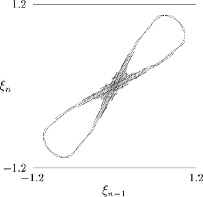
Figure 1: Homoclinic tangles for the two-dimensional map $f$ with $\nu_{1}=1.25$ and $\kappa_{1}=1$, drawn using the software Dynamics NY97 . The circle “$\bullet$” represents the saddle at the origin.

Let $N>0$ be a sufficiently large integer, and let $(\bar{\chi}_{-N},\bar{\xi}_{-N})$ be a point on the unstable subspace such that $(\bar{\xi}_{N+1},\bar{\chi}_{N+1})=(\bar{\chi}_{-N},\bar{\xi}_{-N})$, where $(\bar{\chi}_{N+1},\bar{\xi}_{N+1})=f^{2N+1}(\bar{\chi}_{-N},\bar{\xi}_{-N})$. By the reversibility of $f$, the point $(\bar{\chi}_{N+1},\bar{\xi}_{N+1})$ must be contained in the stable subspace. The two points $(\bar{\chi}_{-N},\bar{\xi}_{-N})$ and $(\bar{\chi}_{N+1},\bar{\xi}_{N+1})$ are also close to the saddle when $N>0$ is large. Hence, the orbit leaving at $(\bar{\chi}_{-N},\bar{\xi}_{-N})$ on the unstable subspace and arriving at $(\bar{\chi}_{N+1},\bar{\xi}_{N+1})$ on the stable subspace is a good approximation to a symmetric homoclinic orbit of $f$. Using an adaptation of the driver HomMap Y98a ; Y98b to AUTO97, we can easily find such approximate homoclinic points.

Now, in order to find non-trivial symmetric homoclinic solutions of $F_{\epsilon}$ for $\epsilon>0$, we take $\epsilon$ as the additional free parameter and choose $(\chi_{-N},\xi_{-N},\epsilon)=(\bar{\chi}_{-N},\bar{\xi}_{-N},0)$ as the starting solution to (34) and (35), where $(\bar{\chi}_{-N},\bar{\xi}_{-N})$ denotes the homoclinic point on the unstable subspace for $f$, obtained using the above procedure. Fixing $\kappa_{1}=1$, we then performed continuation of these algebraic equations in AUTO, using $\delta$ as the continuation parameter. To obtain symmetric homoclinic orbits for $\kappa_{1}=-1$, we also take $\delta$ and $\kappa_{1}$ as the free and continuation parameters, respectively, and continue the solution obtained above for $\kappa_{1}=1$ and $\epsilon=\sqrt{2/(D|\gamma_{1}|)}$. The results are presented in Figs. 2-4. As shown in Figs. 2 and 3, new branches bifurcate from the one with $\epsilon=0$ at discrete values of $\delta$ and can be continued to $\epsilon=\sqrt{2/(D|\gamma_{1}|)}$ by varying $\delta$ and $\epsilon$. As shown in Fig. 4, the branches were also continued from $\kappa_{1}=1$ to $\kappa_{1}=-1$ by varying $\delta$ and $\kappa_{1}$. For $\kappa_{1}=-1$ and $\kappa_{2}=1$, we could not find such symmetric homoclinic orbits of $F_{\epsilon}$ with sufficient precision. In these computations, we also chose the value of $N$ such that the distance between the approximate homoclinic point and the origin was $1.5\times 10^{-3}$ at most, and checked that the results did not change significantly under increase of $N$. Our computations also suggested that a possibly infinite number of branches of symmetric homoclinic orbits could be obtained when $k$ or $q$ is large or $\delta$ is small. These branches show oscillations in the parameter plane, which are sensitive to the value of $N$ and do not appear to converge as $N\rightarrow\infty$. These, probably spurious branches, result from a large ratio between the imaginary eigenvalue of the linearization and the real eigenvalue, which is well known to be a singular limit for equations that bear ES Ch:01 ; Lo:01 , and needs to be treated with great caution. In the results that follow, we have stopped computation at points where such oscillations first become evident, and have checked all results for consistency in the limit of $N\rightarrow\infty$.

Figure 2: Numerical continuation of symmetric homoclinic orbits for $F_{\epsilon}$ when $D=100$ and $N=85$: (a) $k=0.3$, $q=5$ and $\kappa_{1}=\kappa_{2}=1$; (b) $k=0.5$, $q=1$, $\kappa_{1}=1$ and $\kappa_{2}=-1$. Here $\epsilon$ and $\delta$ are varied. The dotted line represents $\epsilon=\sqrt{2/(D|\gamma_{1}|)}$ with $\gamma_{1}=0.05$.

Figure 3: Numerical continuation of symmetric homoclinic orbits for $G_{\epsilon}$ when $D=10$, $k=3$, $q=1$ and $N=15$. Here $\epsilon$ and $\delta$ are varied. The dotted line represents $\epsilon=1$.

Figure 4: Numerical continuation of symmetric homoclinic orbits for $F_{\epsilon}$ when $D=100$, $k=0.5$, $q=1$, $\kappa_{2}=-1$, $N=85$ and $\epsilon=0.6324555\approx\sqrt{2/\left(D|\gamma_{1}|\right)}$ with $\gamma_{1}=0.05$. Here $\delta$ and $\kappa_{1}$ are varied. The dotted line represents $\kappa_{1}=-1$.

VI Numerical results

We now present continuation results obtained with AUTO for symmetric homoclinic orbits of $F_{\epsilon}$ (or $G_{\epsilon}$) under simultaneous variation of two relevant parameters within the saddle-center parameter regions. By varying the discreteness coefficient $D$ up to large values, we are also able to compare the results to those of the continuum limit, $D\rightarrow\infty$. We shall treat the cases $\delta>0$ and $\delta<0$ separately and also discuss the possibility of discrete ESs in the absence of cubic nonlinearity.

VI.1 The case of $\delta>0$

Figure 5 depicts branches of discrete ESs in the presence of $\chi^{(3)}$ terms, with $\gamma_{1}=\gamma_{2}=0.05$ and $k=0.3$. Two distinct branches of ESs are displayed. Along each branch, the profile changes continuously. Figure 6 displays an array of profiles of these ESs for $D=100$ and $D=5$. Note that the second (higher-$\delta$) branch can be considered to be a family of fundamental, i.e. single-humped, solitons throughout the range of existence, whereas the double-humped structure of the SH component of the first branch becomes evident for small $q$. This property, and the location of the branches in the $(\delta,q)$ plane, are fully consistent with results obtained in the continuum limit (ChMaYaKa:01, , Fig. 3). Our numerical results also suggest that there may exist further branches for lower $\delta$-values, each subsequent one containing more oscillations in core of the SH component. However, computation becomes unreliable beyond the first two branches for the reasons given at the end of the last section, and so we do not display those results here. Also experience from the continuum model suggests that non-fundamental ESs never have a chance to be stable.

Figure 5: Branches of the discrete ES solutions for $k=0.3$ and $\gamma_{1}=\gamma_{2}=0.05$. (a) Solutions in the $(\delta,q)$-plane for $(D,N)=(100,86)$ (solid line) $(10,31)$ (dashed line) and $(5,23)$ (broken line). According to (23) ESs also exist only above the dotted line $q=0.6$ for this $k$-value. Labeled points correspond to the relevant subpanels of Fig. 6 where solutions profiles are displayed. (b) Solutions in the $(D,\delta)$-plane for $q=5$ and $N=22$. Note that, according to (23), we must have $\delta D>2.2$ (the boundary is shown as a dotted line).

Figure 6: Profiles of the discrete ESs corresponding to the labeled points in Fig. 5(a): (a) $\delta=0.58637$ and $q=5$; (b) $\delta=2.9894$ and $q=5$; (c) $\delta=0.65467$ and $q=0.6$; (d) $\delta=3.3693$ and $q=0.6$; (e) $\delta=1.3496$ and $q=5$; (f) $\delta=3.1432$ and $q=5$; (g) $\delta=0.80213$ and $q=0.6$; (h) $\delta=3.3824$ and $q=0.6$. In panels (a)-(d), $D=100$ and $N=85$, and in panels (e)-(h), $D=5$ and $N=22$. In this and all subsequent plots, the FF ($u$-component) is interpolated by a solid line and the SH ($v$-component) by a broken line.

Figure 5(b) depicts continuation in $D$ of the solutions on these two branches for $q=5$. In this case, we find that there is a lower limit on $D$ beyond which no ESs exist. This corresponds to the right-hand inequality in the first condition in (23).

We will now check the validity of the analytical approximation developed in Section 3 when $\tilde{k}$ and hence $k$ are large. In Fig. 7, we display the two numerically computed ES branches with the same values of $\gamma_{1}$ and $\gamma_{2}$ as those in Fig. 5 for $D=10$ when $k$ is rather large, and compare them with the analytical prediction (17), taking into regard the relations (22). In Fig. 7(a), the parameters $\delta$ and $k$ are varied with $q=2k$, and in Fig. 7(b) the parameters $\delta$ and $q$ are varied for $k=50$. The analytical predictions are plotted as dashed lines. We find good agreement between the numerical and analytical results, especially for large $k$. Figure 8 displays the profiles of these ESs. The fundamental soliton in Fig. 8(a) has a steep peak at $n=0$, as assumed in the approximate analysis of Section 3.

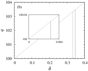
Figure 7: Branches of discrete ESs for $\gamma_{1}=\gamma_{2}=0.05$ and $D=10$; $N=7$ is chosen for larger $\delta$, and $N=5$ for smaller $\delta$. The analytical prediction given by Eqs. (17) and (22) is plotted as a dashed line. (a) Solutions in the $(\delta,k)$-plane for $q=2k$. (b) Solutions in the $(\delta,q)$-plane for $k=50$. The ESs exist in the region $100<q<100+10\delta$, whose boundary is shown as a dotted line.

Figure 8: Examples of the ESs on solution branches in Fig. 7(b): (a) $\delta=0.34718$, $q=102$ and $N=7$; (b) $\delta=0.0029014$, $q=100.02$ and $N=5$.

It is well known that in the continuum case multi-pulse homoclinic orbits exist (under a mild Birkhoff signature condition MiHoOR:92 ; KoChBuSa:02 ) along families of curves in the parameter plane that accumulate on the curves of the fundamental ES solutions. Unlike the branches computed above, they do not feature a single-humped shaped in either component, but rather look like bound-states of two spatially separated fundamental solitons. We have found exactly the same solution families in the discrete model too. An example is presented in Fig. 9.

Figure 9: A typical example of a two-pulse bound state ES in the lattice system (21) with $\delta=1.1261$, $\gamma_{1}=\gamma_{2}=0.05$, $D=5$, $k=0.3$, $q=7$ and $N=51$.

VI.2 The case of $\delta<0$

Figure 10 shows ES branches in the case of self-defocusing $\chi^{(3)}$ terms, with $\gamma_{1}=\gamma_{2}=-0.05$ and $\delta<0$. Figures 11 and 12 display the profiles of these ESs for $D=100$, $D=10$ and $D=6$. Note that these curves and the solutions on them for $D=100$ are identical, to the accuracy depicted, to the corresponding ones found in the continuum counterpart of the model in Ref. (YaMaKaCh:01, , Figs. 2,3).

Figure 10: Branches of ESs in the discrete system (2) with $q=1$ and $\gamma_{1}=\gamma_{2}=-0.05$: (a) In the $(\delta,k)$-plane for $D=100$ and $10$; (b) in the $(D,k)$-plane for $\delta=-0.5$ and $N=30$. In panel (a), the solid and dashed curves represent the results for $D=100$ and $10$, respectively. When $D=100$ (resp. $D=10$), $N=85$ (resp. $N=30$) were used for the most part but $N=93$ or $N=109$ (resp. $N=35$ or $N=40$) were used for the two outer curves with large $|\delta|$. According to condition (23), ESs exist only above $k=0.5$ and below $k=0.5-\delta D$, when $q=1$.

Notice the variety of multi-humped shapes of the solitons belonging to these families. Like the continuum model, only the inner-most of these branches represents a fundamental soliton. Continuation towards the anti-continuum limit, $D\rightarrow 0$, becomes numerically problematic for these solitons. It was found difficult to compute the solutions with repeatable accuracy while varying $N$ below $D\approx 6$. Clearly, these branches become increasingly spiky as $D$ is decreased (see Fig. 12), and it may happen that branches of ES solutions actually terminate before they reach the minimum value of $D$ at which they remain embedded, which would be $D_{\min}=2k-1$, for the values of $q$ and $\delta$ used in Fig. 10(b).

Figure 11: ESs on the branches in Fig. 10(a) for $\delta=-1$: (a) $k=0.69564$; (b) $k=0.71312$; (c) $k=0.71383$; (d) $k=0.71387$; (e) $k=0.6895$; (f) $k=0.70811$; (g) $k=0.70898$; (h) $k=0.70902$. In panels (a)-(d), $D=100$ and $N=85$, and in panels (e)-(h), $D=10$ and $N=30$.

Figure 12: ESs at the end of the above two branches in Fig. 10(b) for $D=6$: (a) $k=0.78427$; (b) $k=0.78426$.

Figure 13 shows the ES branches in a still more exotic case of opposite signs in front of the FF and SH $\chi^{(3)}$ SPM terms, $\gamma_{1}=0.05$ and $\gamma_{2}=-0.05$. This case may, in principle, also be physically relevant – not to ordinary optical materials, but rather to photonic crystals (see, e.g., PhotCryst and references therein). Figure 14 displays the profiles of these ESs for $D=100$ and $D=10$. Note similarity with the branches in Fig. 10 for small $\delta$. However, in this case it is found that the solution branches still exist for large $k$, rather than undergoing turning back with the increase of $k$. Also the internal oscillations on the non-fundamental branches become far less pronounced.

Figure 13: Branches of ESs with $q=1$, $\gamma_{1}=0.05$ and $\gamma_{2}=-0.05$: (a) In the $(\delta,k)$-plane for $D=100$ and $10$; (b) in the $(D,k)$-plane for $k=1$ and $N=24$. In panel (a), the solid and dashed curves represent the results for $D=100$ and $10$, respectively. When $D=100$ (resp. $D=10$), $N=85$ (resp. $N=30$) was used. In panel (b), the forth solid line from the bottom still exists although it is very short and almost invisible. The ESs exist only in the region $0.5<k<0.5-\delta D$ when $q=1$, whose boundary is indicated by a dotted line.

Figure 14: Examples of ESs on the branches in Fig. 13(a) for $k=1$: (a) $\delta=-0.23601$; (b) $\delta=-0.099245$; (c) $\delta=-0.053237$; (d) $\delta=-0.033776$; (e) $\delta=-0.24838$; (f) $\delta=-0.13304$; (g) $\delta=-0.096003$; (h) $\delta=-0.05109$. In panels (a)-(d), $D=100$ and $N=85$; in panels (e)-(h), $D=10$ and $N=30$.

The approximate analysis of Section 3 is also valid for $\gamma_{1}>0$ and $\gamma_{2},\,\delta<0$ when $k$ is large. Figure 15 shows the fundamental ES branch (the left one in Fig. 13(a)) with the same values of $\gamma_{1}$ and $\gamma_{2}$ as those in Fig. 13 for $D=10$ when $k$ is rather large. In Fig. 15(a), the parameters $\delta$ and $k$ are varied for $q=2k$, and in Fig. 15(b) the parameters $\delta$ and $q$ are varied for $k=50$, as in Figs. 7(a) and (b). The predictions based on Eqs. (17) with (22) are plotted as dashed lines. A profile of the ES is also displayed in Fig. 15(a). We see that Eq. (17) again approximates well the numerical result for the fundamental solitons when $k$ is large. The ES in Fig. 15(a) features a steep peak at $n=0$, as assumed in the analytical approximation.

Figure 15: Branches of discrete ESs for $\gamma_{1}=0.05$, $\gamma_{2}=-0.05$, $D=10$ and $N=7$. The analytical prediction, given by Eqs. (17) and (22) is plotted by dashed lines. (a) Solutions in the $(\delta,k)$-plane for $q=2k$. (b) Solutions in the $(\delta,q)$-plane for $k=50$. The ESs exist in the region $100+10\delta<q<100$, whose boundary is shown by the dotted line. An example of the ES, for $\delta=-0.31873$ and $q=98$, is plotted in panel (b).

Finally, we briefly discuss the case in which $\gamma_{1}=\gamma_{2}=0$, i.e., the $\chi^{(3)}$ terms are absent. As shown in Fig. 16, we could follow solutions of the three-dimensional algebraic problem for $G_{\epsilon}$. However, these solutions do not represent ESs since the origin is not a saddle-center but a hyperbolic saddle. Although the region $q/2<k<q/2-\delta D$ in which the origin is a saddle-center becomes wider when $D$ is larger, for the solution $k$ diverges to $\infty$ as $D\rightarrow\infty$. Thus, there seems to be no hope that an ES exists in this case. As mentioned above, this situation is very similar to that in the continuum model (1).

Figure 16: Branches of solutions of the three-dimensional algebraic problem for $G_{\epsilon}$ in the absence of the $\chi^{(3)}$ nonlinearity, with $\gamma_{1}=\gamma_{2}=0$, and $q=1$. (a) In the $(\delta,k)$-plane for $D=10$; (b) in the $(D,k)$-plane for $\delta=-0.1$ and $N=15$. In panel (a), $N=15$ and $25$ were used for $k>1$ and $k<1$, respectively. The ESs would exist only in the region $0.5<k<0.5-\delta D$, the boundaries of which are plotted as dotted lines, when $q=1$. An example of a non-embedded (gap) soliton, found in this case for $\delta=-0.1$ and $k=1.9027$, is plotted in panel (a).

VII Conclusions

In this paper, we have established the existence of embedded solitons (ESs) in the discrete model of the second-harmonic generation in the presence of cubic nonlinearity. The model can be naturally realized as an array of channel waveguides in the spatial domain, therefore our results suggest possibilities for new experiments with discrete spatial solitons in nonlinear optics. We have also introduced a simplified model, with the $\chi^{(3)}$ nonlinearity present solely at the central site, in which the existence of an ES was demonstrated in an asymptotic analytical form. In the general case, the existence region for the ESs in the discrete model was found numerically. Moreover, we have checked that the asymptotic analysis of the simplified model in the limit of large wavenumbers gives a good approximation of the codimension-one set in parameter space, on which the ESs exist.

More generally, we have established, that unlike the discretizations of other (dissipative) continuum models bearing localized solutions, the codimension of ESs does not change when one passes to a discrete version. Whereas continuum ESs may be regarded as homoclinic orbits to saddle-center equilibria in reversible flows (ordinary differential equations), discrete ESs should be thought of as homoclinic orbits to saddle-center fixed points of reversible maps. Both have codimension one in the parameter space. Understanding this property led us to the derivation of a numerical method for computing homoclinic orbits to nonhyperbolic equilibria of reversible maps.

Accurate investigation of stability of ESs in the lattice model is beyond the scope of the present investigation. Systematic results for the stability will be presented elsewhere; however, some preliminary results suggest that the fundamental discrete ESs inherit the semi-stability property found in the corresponding continuous model YaMaKaCh:01 ; PeYa:02 . We expect that general arguments in favor of the semi-stable character of these solitons for the continuous case should apply in the discrete setting as well.

Figure 17 shows a preliminary computational result for $D=10$, $\delta=-1$, $k=0.6895$, $q=1$ and $\gamma_{1}=\gamma_{2}=-0.05$, corresponding to the fundamental ES of Fig. 11(e). Here Eq. (2) was integrated numerically by the fourth-order Runge-Kutta method under the boundary condition

$$u_{-\bar{N}-1}(z)=u_{\bar{N}+1}(z)=v_{-\bar{N}-1}(z)=v_{\bar{N}+1}(z)=0$$ (37)

for all $z\geq 0$ with $\bar{N}=93$ and the initial condition

$$u_{n}(0)=(1+c_{1})U_{n},\quad v_{n}(0)=(1+c_{2})V_{n}$$ (38)

where $(U_{n},V_{n})$ represents an approximate ES given by the data of Fig. 11(e) for $|n|\leq N=30$ and by $U_{n}=V_{n}=0$ for $|n|>N$, and $c_{1,2}$ are small amplitudes of the initial disturbance, which were chosen to be $c_{1}=c_{2}=0.01$. The positive values of $c_{1,2}$ mean that the norm

$$E=\sum_{n=-\bar{N}}^{\bar{N}}(|u_{n}|^{2}+2|v_{n}|^{2})$$ (39)

of the perturbed state (in the temporal-domain optical model, it plays the role of energy) is greater than that of the unperturbed ES. In Fig. 17 we see the characteristic hallmark of semi-stability for the ES: The shapes of the perturbed wave are almost unchanged for a long period of $t$ in Figs. 17(a) and(b), and the amplitudes $|u_{0}(t)|$ and $|v_{0}(t)|$ exhibit small oscillations near the unperturbed values in Figs. 17(c) and(d). However, the perturbed ES was destroyed in the simulations when different signs of $c_{1}$ and $c_{2}$ were chosen. Further investigation of stability and bifurcation will be the subject of future work.

Figure 17: Evolution of the fundamental ES (corresponding to Fig. 11(e)) initiated by the nondestructive perturbation with $c_{1}=c_{2}=0.01$ in the initial conditions (38). The dashed lines in panels (c) and (d) are the amplitudes of the $u_{0}$- and $v_{0}$-components of the unperturbed soliton.

Finally, our results so far pertain only to those discrete ESs that are symmetric with respect to the involution $R$ defined in Eq. (28); solitons with this symmetry have an on-site central peak. It is also possible to apply techniques developed in this work to solutions symmetric with respect to involution $\hat{R}$, see Eq. (29), that should feature an inter-site central peak. In other physical context, such waves are less likely to be stable than waves that are centered on a lattice site Review . However, that understanding typically applies to regular (gap) discrete solitons and need not necessarily apply to ESs. We shall address this issue in future work.

References

References

- (1) Yang J, Malomed B A and Kaup D J 1999 Embedded solitons in second-harmonic-generating systems Phys. Rev. Lett. 83 1958–1961
- (2) Champneys A R, Malomed B A, Yang J and Kaup D J 2001 Embedded solitons: Solitary waves in resonance with the linear spectrum Physica D 152-153 340–354
- (3) Yang J, Malomed B A, Kaup D J and Champneys A R 2001 Embedded solitons: A new type of solitary wave Math. Comp. Sim 56 585–600
- (4) Champneys A R and Groves M D 1997 A global investigation of solitary waves solutions to a two-parameter model for water waves J. Fluid. Mech. 342 299–229
- (5) Fujioka J and Espinosa A 1997 Soliton-like solution of an extended NLS equation existing in resonance with linear dispersive waves J. Phys. Soc. Jpn. 66 2601–2607
- (6) Champneys A R, Malomed B A and M. J. Friedman 1998 Thirring solitons in the presence of dispersion Phys. Rev. Lett. 80 4168–4171
- (7) Atai J and Malomed B A 2001 Solitary waves in systems with separated Bragg grating and nonlinearity Phys. Rev. E 64 066617
- (8) Kolossovski K, Champneys A R, Buryak A and R. A. Sammut 2002 Multi-pulse embedded solitons as bound states of quasi-solitons Physica D 171 153–177
- (9) Espinosa-Ceron A, Fujioka J and Gomez-Rodriguez A 2003 Embedded solitons: Four-frequency radiation, front propagation and radiation inhibition Physica Scripta 67 314–324
- (10) Yang J K 2003 Stable embedded solitons Phys. Rev. Lett. 91 143903
- (11) Mak W C K, Malomed B A and Chu P L 2004 Symmetric and asymmetric solitons in linearly coupled Bragg gratings Phys. Rev. E 69 066610
- (12) Merhasin I M and Malomed B A 2004 Four-wave solitons in Bragg cross-gratings J. Optics B: Quant. Semiclass. Opt. 6 S323-S332
- (13) Pelinovsky D E and Yang J 2002 A normal form for nonlinear resonance of embedded solitons, Proc. Roy. Soc. Lond. A 458 1469–1497
- (14) Champneys A R and Kivshar Yu S 2000 Origin of multikinks in dispersive nonlinear systems Phys. Rev. E 61 2551–2554
- (15) Flach S, Zolotaryuk Y and Kladko K 1999 Moving lattice kinks and pulses: An inverse method Phys. Rev E 59 6105-6115
- (16) Morgante A M, Johansson M, Kopidakis G and Aubry S 2002 Standing wave instabilities in a chain of nonlinear coupled oscillators Physica D 162 53-94
- (17) Peyrard M and Kruskal M D 1984 Kink dynamics in the highly discrete sine-Gordon system Physica D 14 88–102
- (18) Braun O M and Kivshar Yu S 1998 Nonlinear dynamics of the Frenkel-Kontorova model Phys. Rep. 306 1–108
- (19) Savin A V. Zolotaryuk Y and Eilbeck J C 2000 Moving kinks and nanopterons in the nonlinear Klein-Gordon lattice Physica D 138 267–281
- (20) Aigner A A, Champneys A R and Rothos V R 2003 A new barrier to the existence of moving kinks in Frenkel-Kontorova lattices Physica D 186 148–170
- (21) Gonzalez-Perez-Sandi S, Fujioka J and Malomed B A 2004 Embedded solitons in dynamical lattices Physica D 197 86–100
- (22) Fiedler B and Scheurle J 1996 Discretization of Homoclinic Orbits, Rapid Forcing and “Invisible” Chaos Memoirs of Amer. Math. Soc. 119 (Providence RI: American Mathematical Society)
- (23) Bang O, Clausen C B, Christiansen P L and Torner L 1999 Engineering competing nonlinearities Opt. Lett. 24 1413–1415
- (24) Corney J F and Bang O 2001 Solitons in quadratic nonlinear photonic crystals Phys. Rev. E 64 047601
- (25) Johansen S K, Carrasco S, Torner L and Bang O 2002 Engineering of spatial solitons in two-period QPM structures Opt. Commun. 203 393–402
- (26) Etrich C, Lederer F, Malomed B A, Peschel T, and Peschel U 2000 Optical solitons in media with a quadratic nonlinearity Progr. Opt. 41 483-568
- (27) Iwanow R, Schiek R, Stegeman G I, Pertsch T, Lederer F, Min Y and Sohler W 2004 Observation of discrete quadratic solitons Phys. Rev. Lett. 93 113902
- (28) Kevrekidis P G Malomed B A, and Musslimani Z 2003 Discrete gap solitons in a diffraction-managed waveguide array Eur. Phys. J. D 67 013605
- (29) Eisenberg H S, Silberberg Y, Morandotti R, Boyd A and Aitchison J S 2000 Diffraction management Phys. Rev. Lett. 85 1863–1866
- (30) Pertsch T, Zentgraf T, Peschel U and Lederer F 2002 Anomalous refraction and diffraction in discrete optical systems Phys. Rev. Lett. 88 093901
- (31) Devaney R L 1976 Reversible diffeomorphisms and flows Trans. Amer. Math. Soc. 218 89–113
- (32) Lamb J S W and Roberts J A G 1998 Time-reversal symmetry in dynamical systems: A survey Physica D 112 1–39
- (33) Guckenheimer J and Holmes P 1983 Nonlinear Oscillations, Dynamical Systems, and Bifurcations of Vector Fields (New York: Springer)
- (34) Doedel E, Champneys A R, Fairgrieve T F, Kuznetsov Y A, Sandstede B and Wang X 1997 AUTO97: Continuation and Bifurcation Software for Ordinary Differential Equations (with HomCont) Available by anonymous ftp from ftp.cs.concordia.ca, directory pub/doedel/auto
- (35) Nusse E H and Yorke J A 1997 Dynamics: Numerical Explorations 2nd ed. (New York: Springer)
- (36) Kawakami H 1981 Algorithme numérique définissant la bifurcation d’un point homocline C. R. Acad. Sc. Paris, Série I 293 401–403
- (37) Beyn W-J and Kleinkauf J N 1997 The numerical computation of homoclinic orbits for maps SIAM J. Num. Anal. 34 1207–1236
- (38) Beyn W-J and Kleinkauf J N 1997 Numerical approximation of homoclinic chaos Numer. Algorithms 14 25–53
- (39) Yagasaki K 1998 Numerical detection and continuation of homoclinic points and their bifurcations for maps and periodically forced systems Int. J. Bifurcation Chaos 7 1617–1627
- (40) Bergamin J M, Bountis T and Vrahatis M N 2002 Homoclinic orbits of invertible maps Nonlinearity 15 1603–1619
- (41) Yagasaki K 1998 HomMap: An Auto driver for homoclinic bifurcation analysis of maps and periodically forced systems (Gifu Japan: Gifu University)
- (42) Lombardi E 2000 Oscillatory Integrals and Phenomena beyond All Algebraic Orders: With Applications to Homoclinic Orbits in Reversible Systems (Berlin: Springer)
- (43) Champneys A R 2001 Codimension-one persistence beyond all orders of homoclinic orbits to singular saddle centers in reversible systems Nonlinearity 14 87–112
- (44) Mielke A, Holmes P and O’Reilly O 1992 Cascades of homoclinic orbits to, and chaos near, a Hamiltonian saddle-center J. Dyn. Diff. Eqns. 4 95–126
- (45) Andreani L C, Agio M, Bajoni D, Belotti M, Galli M, Guizzetti G, Malvezzi A M, Marabelli F, Patrini M and Vecchi G 2003 Morphology and optical properties of bare and polydiacetylenes-infiltrated opals Synthetic Metals 139 695–700