Spectral correlations of individual quantum graphs

Abstract

We investigate the spectral properties of chaotic quantum graphs. We demonstrate that the ‘energy’–average over the spectrum of individual graphs can be traded for the functional average over a supersymmetric non–linear $\sigma$–model action. This proves that spectral correlations of individual quantum graphs behave according to the predictions of Wigner–Dyson random matrix theory. We explore the stability of the universal random matrix behavior with regard to perturbations, and discuss the crossover between different types of symmetries.

I Introduction

The spectral fluctuations of individual complex (chaotic) quantum systems are universal and can be described in terms of Wigner–Dyson random matrix theoryWigner ; Dyson . (See also Mehta ; Guhr ; Haake ; Stockmann ; Efetov and references therein). For classically chaotic systems this empirical statement was promoted to a conjecture by Bohigas, Giannoni and Schmit BGS . (See also Casati ; Berry_anp .) While, however, there is enormous experimental and numerical evidence in support of this conjecture exceptions the physical basis of universality is not yet fully understood theoretically.

To date, the most advanced approach in developing correspondences between spectral statistic and non–linear dynamics is semiclassical analysis. Beginning with Berry’s seminal work Berry_diagonal it became understood that information on spectral correlations is stored in action correlations of classical periodic orbits (see also action_correlations .) Going beyond the ‘diagonal’ approximation Berry_diagonal wherein only identical (and mutually time–reversed) orbits contributing to the Gutzwiller double sum Gutzwiller are taken into account, a hierarchy of ever more complex expansions in orbit pairs has been constructed SR ; tau_2 ; tau_infinity . In this way, it was shown that to all orders in an expansion in the ratio $\tau\equiv t/t_{H}$ the short time ($t<t_{H}$) behavior of the spectral form factor $K(\tau)$ of uniformly hyperbolic quantum systems coincides with the universal predictions of random matrix theory (RMT). (Here, $t_{H}=\frac{2\pi\hbar}{\Delta E}$ denotes the Heisenberg time and $\Delta E$ is the mean level spacing.) However, in view of the fact that at $\tau=1$, the function $K(\tau)$ contains an essential singularity, it is presently not clear how to extend this expansion to times larger than the Heisenberg time.

Some time ago, a field theoretical approach to quantum chaos — dubbed the ballistic $\sigma$–model — has been introduced AAA as an alternative to semiclassical expansions. The most promising aspect of this development is that in field theory the full information on universal RMT correlations is obtained in a very simple manner, viz. by integration over globally uniform ‘mean field’ configurations; universality of chaotic quantum systems is proven, once it has been shown that at sufficiently low energies (long times) fluctuations become negligible and the field theory indeed reduces to its mean field sector. Unfortunately, however, it has so far not been possible to demonstrate this reduction in a truly convincing manner. (The situation is much better in the field of disordered chaotic systems: It has been known for some time that at low energies disordered systems exhibit RMT spectral correlations upon configurational averaging. This type of universality has been proven Efetov by field theoretical methods similar to those mentioned above.)

Motivated by the lack of universality proofs for generic quantum systems with underlying Hamiltonian chaos, we have recently considered the spectral properties of quantum graphs GA . (For the general theory of quantum graphs, see Kuchment and references therein.) Quantum graphs differ from generic Hamiltonian systems in two crucial aspects: First, the classical dynamics on the graph is not deterministic. It is rather described by a Markov process. Second, quantum graphs are ‘semiclassically exact’ in that their spectrum can be exactly described in terms of trace formulae. In spite of these differences, quantum graphs display much of the behavior of generic hyperbolic quantum systems Kottos (while being not quite as defiant to analytical treatment than these.)

Earlier work on universal spectral statistics in quantum graphs was based on periodic orbit summation schemes similar in spirit to the semiclassical approach to Hamiltonian systems. Specifically, Berkolaiko et al. greg developed a perturbative diagrammatic language to analyze the periodic–orbit expansions of spectral correlation functions beyond the diagonal approximation. Tanner Tanner analyzed the structure of the semiclassical expansion to conjecture criteria for the presence of universal correlations on graphs. He also established connections between universality and the decay rates of classical Markovian dynamics of the system (for details see appendix A).

While all building blocks of semiclassical analysis on graphs are known greg ; GS , and a complete summation over all orbit pairs may be in reach, semiclassics on graphs is subject to the same limitations as in Hamiltonian systems. In particular, it is not clear how to extend its domain of applicability to times beyond the Heisenberg time. In view of these difficulties, we have developed an alternative approach GA which is based on field theoretical methods and avoids diagrammatic resummations altogether. Rather, it is based on two alternative pieces of input, both of which have been discussed separately before:

• The exact equivalence of a spectral average for a quantum graph with incommensurate bond lengths to an average over a certain ensemble of unitary matrices Kottos ; Barra ; Tanner .

• An exact mapping of the phase–averaged spectral correlation functions onto a variant of the supersymmetric $\sigma$–model by an integral transform known as the color–flavor transformation Zirnbauer .

The synthesis of i. and ii. GA leads to a formulation similar in spirit to the ‘ballistic $\sigma$–model’ yet not burdened by the technical problems of that approach. It is the purpose of this paper to give a detailed account of this theory, and to discuss a number of generalizations. Specifically, we will discuss the crossover between systems of conserved (orthogonal symmetry) and broken (unitary symmetry) time–reversal invariance, and we will consider the case of broken spin rotation invariance (symplectic symmetry.)

The paper is organized as follows: In Section II we give a short introduction to quantum graphs. We discuss the relevant quantization conditions, spectral correlators, and the meaning of incommensurate bond lengths. The supersymmetry approach to the spectral two–point correlation function is discussed in Section III. In Section IV we subject the supersymmetric generating functional to a stationary phase analysis. We show under which conditions the field theory can be reduced to a ‘mean field’ theory of RMT–type correlations. We also discuss the crossover between graphs of orthogonal and unitary symmetry. Quantum graphs belonging to the symplectic symmetry class are discussed in appendix B, and an outline of the proof of the color–flavor transformation is given in appendix C.

II Quantum graphs

II.1 Generalities

A finite graph ${\mathcal{G}}$ consists of $V$ vertices which are connected by $B$ bonds. The $V\times V$ connectivity matrix is defined by

$$C_{i,j}=\#\left\{\textrm{bonds connecting the vertices $i$ and $j$}\right\}.$$ (1)

A graph is simple if for all $i,\ j$, $C_{i,j}\in[0,1]$ (no parallel connections) and $C_{i,i}=0$ (no loops). The number of bonds is $B=\frac{1}{2}\sum_{i,j=1}^{V}C_{i,j}$. The valency of a vertex $i$ is the number of bonds connected to it $v_{i}=\sum_{j=1}^{V}C_{i,j}$. A graph is called ‘connected’ if it cannot be split into disjoint sub–graphs. With only slight loss of generality fn:simple , we will focus on the case of simple connected graphs throughout (cf. Fig. 1 for a schematic.)

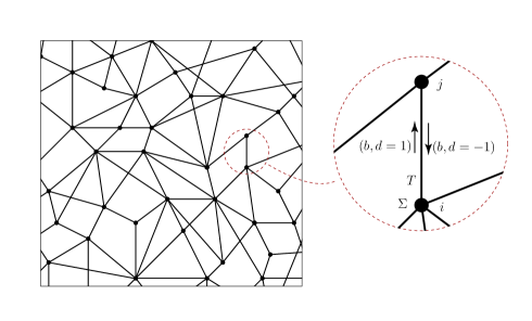
Figure 1: Schematic of a fraction of a (planar) simple quantum graph and of the notation used in the text.

We denote a bond connecting the vertices $i$ and $j$ by $b=(ij)$. The notation $(ij)$ and the letter $b$ will be used whenever we refer to bonds without specifying a direction: $b\in(ij)=(ji)$. A directed bond $\beta=(b,d)$ consists of a bond $b$ and a direction on the bond which will be denoted by a direction index $d=\pm 1$. For $b=(ij)$ and $i<j$ we set $d=+1$ for the direction $i\rightarrow j$ and $d=-1$ on the opposite direction.

The position $x$ of a point on the graph is determined by specifying its bond $b$, and its distance $x_{b}\in[0,L_{b}]$ from the adjacent vertex with the smaller index. The length of a bond is denoted by $L_{b}$. Throughout, we will assume the bond lengths to be incommensurable (or rationally independent) in the sense that there is no non–vanishing set of integers $m_{b}\in\mathbbm{Z}$ such that $\sum_{b}m_{b}L_{b}=0$.

The Schrödinger operator on ${\mathcal{G}}$ is defined by one–dimensional Laplacians on the bonds, and a set of vertex boundary conditions establishing self–adjointness. Its wave functions $\Psi(x)$ are complex valued, piecewise continuous and bounded functions. Writing $\Psi(x)\equiv\psi_{b}(x_{b})$ for $x=x_{b}\in(0,L_{b})$, the solutions of the stationary Schrödinger equation at a given wave number $k>0$ have the form

$$\begin{split}&\psi_{b}(x_{b};k)=e^{-iA_{b}(x_{b}-\frac{L_{b}}{2})}\times\\ &\qquad\left(\alpha_{b,+1}e^{ik(x_{b}-\frac{L_{b}}{2})}+\alpha_{b,-1}e^{-ik(x_{b}-\frac{L_{b}}{2})}\right),\end{split}$$ (2)

where $\alpha_{b,d=\pm 1}$ are the complex amplitudes of ‘right’ ($d=+1$) and ‘left’ ($d=-1$) propagating waves on the bond, and $A_{b}$ are constant phases generated by optional magnetic fluxes threading the plaquettes of the graph. To characterize the vertex boundary conditions, we introduce ($k$–independent) $v_{i}\times v_{i}$ vertex scattering matrices $\Sigma^{(i)}_{b,b^{\prime}}$ connecting incoming waves to outgoing waves at $i$. ($b$ and $b^{\prime}$ run over bonds connected to $i$). Denoting the outgoing/incoming direction on bond $b$ by $d_{\mathrm{out}}$/$d_{\mathrm{in}}$, these matrices are defined by the equation

$$\begin{split}&\alpha_{bd_{\mathrm{out}}}e^{-i(k-d_{\mathrm{out}}A_{b})\frac{L_{b}}{2}}=\\ &\qquad\qquad\sum_{b^{\prime}}\Sigma^{(i)}_{b,b^{\prime}}e^{i(k-d_{\mathrm{in}}A_{b^{\prime}})\frac{L_{b^{\prime}}}{2}}\alpha_{b^{\prime}d_{\mathrm{in}}},\end{split}$$ (3)

To represent this equation in a more concise form, we combine all amplitudes $\alpha_{bd}$ into a $2B$-dimensional vector $\vec{\alpha}$. In this notation,

$$\vec{\alpha}=\mathcal{U}_{B}(k)\vec{\alpha}$$ (4)

where the $2B\times 2B$ quantum map bondscattering is given by

$$\mathcal{U}_{B}(k)=T(k)ST(k),$$ (5)

the diagonal matrix $T(k)_{b\,d,b^{\prime}\,d^{\prime}}=\delta_{b\,d,b^{\prime}\,d^{\prime}}e^{i(k+dA_{b})L_{b}/2}$ describes the propagation along half a bond, and

$$S_{bd,b^{\prime}d^{\prime}}=\begin{cases}\Sigma^{(i)}_{b,b^{\prime}}&\text{$(b^{\prime},d^{\prime})\rightarrow i\rightarrow(b,d)$}\\ 0&\text{else},\end{cases}$$ (6)

combines all boundary conditions at the vertices into a single scattering matrix. The equivalent of the quantum map in a Hamiltonian system is a quantized Poincaré map.

The boundary condition (4) can be fulfilled only for discrete set of wave numbers $k_{n}$. These numbers define the spectrum of the quantum graph. For $k>0$ the quantization condition (4) is equivalent to the vanishing of the spectral determinant

$$\xi(k)\equiv\mathrm{det}\left(\mathbbm{1}-\mathcal{U}_{B}(k)\right).$$ (7)

Thus $\xi(k)=0$ if and only if $k=k_{n}>0$ is in the spectrum.

By way of example, we mention two frequently employed families of boundary conditions: so–called Neumann boundary conditions neumann correspond to

$$\Sigma^{(i),\mathrm{N}}_{b,b^{\prime}}=\frac{2-\delta_{b,b^{\prime}}v_{i}}{v_{i}}.$$ (8)

For large valencies $v_{i}$ the non-diagonal terms are much smaller than the diagonal, and the back scattering term dominates. While on general graphs wave functions need not be continuous across the vertices, they are so on Neumann graphs Kottos . Another interesting set of boundary conditions is implemented through discrete Fourier transform (DFT) matrices

$$\Sigma^{(i),\mathrm{DFT}}_{b,b^{\prime}}=\frac{1}{\sqrt{v_{i}}}\exp\left(2\pi i\frac{\hat{\pi}(b)\hat{\pi}(b^{\prime})}{v_{i}}\right)$$ (9)

where $b\mapsto\hat{\pi}(b)$ maps the $v_{i}$ bonds connected to vertex $i$ one-to-one onto the numbers $1,2\dots,v_{i}$. These boundary conditions do not imply continuity at the vertices; incoming wave packets are scattered into the outgoing bonds with equal probability.

II.2 Time–reversal invariance

As with Hamiltonian chaotic symmetries, quantum graphs of different symmetries may be identified. Specifically, quantum graphs carrying spin degrees of freedom (and spin–rotation invariance breaking vertex scattering matrices) fall into the symplectic or unitary symmetry class depending on whether time reversal invariance is broken or not. These cases will be discussed in appendix B. In the absence of spin, we need to distinguish between graphs with broken (unitary symmetry or symmetry class $A$ in the notation of AZ ) or conserved (orthogonal symmetry or symmetry class $A$I) time reversal invariance.

A quantum system is time–reversal invariant if its Hamiltonian $H$ commutes with an anti–unitary time–reversal operator $\mathcal{T}$, $\left[H,\mathcal{T}\right]=0$. For spinless systems, $\mathcal{T}$ is an involutory operator, $\mathcal{T}^{2}=\mathbbm{1}$Haake . The condition $\left[H,\mathcal{T}\right]=0$ restricts the form of both the bond propagation matrix $T(k)$ and the vertex scattering matrices $\Sigma(k)$. In non–time reversal invariant systems, these matrices obey no conditions other than unitarity. However, for conserved time reversal invariance, and with a definitive choice of the time–reversal operator $\mathcal{T}$, all vertex scattering matrices have to be symmetric $\Sigma^{(i)}=\Sigma^{(i)\;T}$, i.e.

$$S=S^{\mathcal{T}}\equiv\sigma^{\mathbf{dir}}_{\mathrm{1}}S^{T}\sigma^{\mathbf{dir}}_{\mathrm{1}}$$ (10)

where $\sigma^{\mathbf{dir}}_{\mathrm{1}}=\left(\begin{smallmatrix}0&\mathbbm{1}\\ \mathbbm{1}&0\end{smallmatrix}\right)$ is the Pauli matrix in direction indices $d$. Additionally, all magnetic phases $A_{b}$ must vanish. The crossover between orthogonal and unitary symmetry will be discussed in IV.3 where we explore the consequences of a gradual switching on of magnetic phase factors.

II.3 The density of states and spectral correlation functions of quantum graphs

The density of states (DoS) of a quantum graph is defined as

$$d(k)=\sum_{n}\delta(k-k_{n})=\frac{1}{\Delta}+\delta d(k)$$ (11)

where the sum runs over the spectrum $k_{n}$. We have written the DoS as a sum over a smooth part $1/\Delta$ where $\Delta$ is the mean level spacing and fluctuations $\delta d(k)$. Both parts allow for an explicit representation in terms of the quantum evolution map. For the mean (or Weyl) part one obtains

$$\frac{1}{\Delta}=\frac{1}{2\pi i}\frac{d}{dk}\mathrm{ln}\,\mathrm{det}\left(-\mathcal{U}_{B}(k)\right)=\frac{B\overline{L}}{\pi},$$ (12)

where $\overline{L}=\frac{1}{B}\sum_{b}L_{b}$ is the mean bond length. Note that the mean level spacing is constant. The fluctuations can be expressed through the spectral determinantKottos

$$\delta d(k)=-\frac{1}{\pi}\mathrm{Im}\,\frac{d}{dk}\mathrm{ln}\,\xi(k^{+}),$$ (13)

where $k^{+}\equiv k+i\epsilon$ and the limit $\epsilon\rightarrow 0$ is implied. Using that $\mathrm{ln}\,\mathrm{det}\,A=\mathrm{tr}\,\mathrm{ln}\,A$ and expanding the logarithm one obtains an exact Gutzwiller type trace formula

$$\delta d(k)=\frac{1}{\pi}\mathrm{Im}\frac{d}{dk}\sum_{n=1}^{\infty}\frac{1}{n}\mathrm{tr\,}\mathcal{U}_{B}^{n}(k^{+})$$ (14)

expressing the DoS in terms of a sum over periodic orbits (periodic sequences of directed bonds.)

We aim to explore the statistical properties of the fluctuating part of the DoS. The $N$-point DoS correlation function is defined by an average over the complete spectrum

$$\begin{split}&R_{N}(s_{1},\dots,s_{N-1})\equiv\\ &\Delta^{N}\left\langle\delta d(k+s_{N-1}\Delta)\dots d(k+s_{1}\Delta)\delta d(k)\right\rangle_{k},\end{split}$$ (15)

where

$$\langle f(k)\rangle_{k}\equiv\lim_{K\rightarrow\infty}\frac{1}{K}\int_{0}^{K}dkf(k).$$ (16)

Throughout, we will focus attention on the two–point correlation function $R_{2}(s)$. The two–point function can be conveniently expressed as a derivative of quotients of spectral determinants:

$$R_{2}(s)=\frac{1}{8g^{2}\pi^{2}}\frac{d^{2}}{dj_{+}dj_{-}}\big{|}_{j=0}\mathrm{Re}\,\left\langle\zeta(j_{+},j_{-};s)\right\rangle_{k},$$ (17)

where

$$\zeta(j_{+},j_{-};s)\equiv\frac{\xi(k^{+}+p_{+\mathrm{\bf f}})}{\xi(k^{+}+p_{+\mathrm{\bf b}})}\left(\frac{\xi(k^{+}+p_{-\mathrm{\bf f}})}{\xi(k^{+}+p_{-\mathrm{\bf b}})}\right)^{*}$$ (18)

and $p_{\pm\mathrm{\bf b}}=(\pm s/2-j_{\pm})\Delta$, $p_{\pm\mathrm{\bf f}}=(\pm s/2+j_{\pm})\Delta$. (Higher order correlation functions may be obtained in a similar manner from generating functions involving additional quotients of spectral determinants.)

For later reference, we recall that the RMT two–point correlation functions are given by

$$\begin{split}R_{2}^{\mathrm{GUE}}(s)=&\delta(s)-\frac{\sin^{2}\pi s}{\pi^{2}s^{2}}\\ R_{2}^{\mathrm{GOE}}(s)=&R_{2}^{\mathrm{GUE}}(s)+\\ &\frac{\left(\pi|s|\cos\pi s-\sin\pi|s|\right)\left(2\,\mathrm{Si}(\pi|s|)-\pi\right)}{2\pi^{2}s^{2}},\end{split}$$ (19)

where $\mathrm{Si}(x)=\int_{0}^{x}dx^{\prime}\,\frac{\sin x^{\prime}}{x^{\prime}}$ is the sine integral.

We also notice that the statistical properties of the graph may be characterized by correlation functions different yet closely allied to the correlation functions introduced above: for any value of $k$ the quantum map $\mathcal{U}_{B}$ possess a set of $2B$ ‘eigenphases’ $e^{-i\theta_{l}(k)}$ ($l=1,\dots,2B$) on the unit-circle. At fixed $k$ the density of phases is given by

$$\rho_{k}(\theta)=\sum_{l=1}^{2B}\delta_{2\pi}(\theta-\theta_{l}(k))$$

where $\delta_{2\pi}(\theta)$ is the $2\pi$-periodic delta–function. The statistical properties of this quantity are defined by averaging over both $\theta$ and $k$. Occasionally — e.g. within the context of the periodic orbit approach to graphs — it is sometimes advantageous to consider the correlation functions of the eigenphases instead of the spectral correlators introduced above. Under mild conditions (weak fluctuations in the bond lengths) both types of correlators are equivalent in the limit $B\rightarrow\infty$ of large graphs. In the following we will keep our discussion focused on the spectral correlators. With small and straight forward changes our theory can be applied to the eigenphase-correlations as well.

II.4 Consequences of incommensurability

The quantum map $\mathcal{U}_{B}(k)=T(k)ST(k)$ depends on the wave number $k$ via the $B$ diagonal elements $e^{ikL_{b}/2}$. Defining $\phi_{b}(k)\equiv kL_{b}/2$ we have a map $k\mapsto(e^{i\phi_{1}(k)},\dots,e^{i\phi_{B}(k)})$ of the wavenumber into a $B$-torus $T^{B}\subset\mathbbm{C}^{B}$. This map may be interpreted as a ‘Hamiltonian flow’ where $k$ plays the role of ‘time’. As we assume incommensurable bond lengths $L_{b}$, the image of the phase map covers the torus densely, i.e. the Hamiltonian flow is ‘ergodic’. This in turn means that long time averages ($k$–averages) may be traded for phase space averages (averages over the torus or, equivalently, independent averages over the $B$ phases $\phi_{b}$ Barra ):

$$\begin{split}\Big{\langle}f\big{(}\{e^{i\phi_{b}(k)}\}\big{)}\Big{\rangle}_{k}=&\Big{\langle}f\big{(}\{e^{i\phi_{b}}\}\big{)}\Big{\rangle}_{\phi}\\ \equiv&\frac{1}{(2\pi)^{B}}\int_{T^{B}}d^{B}\phi\,f\big{(}\{e^{i\phi_{b}}\}\big{)}.\end{split}$$ (20)

It is this equivalence which makes the analytical calculation of spectral correlation functions a feasible task. Upon replacing $\langle\;\rangle_{k}\to\langle\;\rangle_{\phi}$, the one–parameter family of matrices $T(k)\to T(\{\phi_{b}\})$ becomes an ’ensemble’ of random matrices. There is a well developed analytical machinery designed to perform random phase averages of this kind. Below, we will apply the formalism of supersymmetry to compute the random phase averaged spectral correlation functions of the graph which, by virtue of the equivalence above, are strictly equivalent to the wave number averaged correlation functions.

III Nonlinear $\sigma$ model for quantum graphs

Consider the representation (17) of the two–point correlation function in terms of a double derivative of the quotient $\zeta$ of spectral determinants. Replacing the $k$–average by a random phase average, $\langle\zeta\rangle_{k}\to\langle\zeta\rangle_{\phi}$, it is the purpose of the present section to derive a $\sigma$–model representation of the two–point correlation function.

III.1 The generating function as a Gaussian superintegral

Defining the supervectors

$$\psi=\begin{pmatrix}s_{1}\\ \dots\\ s_{N}\\ \chi_{1}\\ \dots\\ \chi_{N}\end{pmatrix}\;\;\text{and}\;\;\tilde{\psi}=\begin{pmatrix}s_{1}^{*}&\dots&s_{N}^{*}&\tilde{\chi}_{1}&\dots\tilde{\chi}_{N}\end{pmatrix},$$ (21)

where $s_{i}$ are complex commuting variables while $\chi_{i}$ and $\tilde{\chi}_{i}$ are independent anti-commuting numbers, the quotient of determinants of an $N\times N$ matrix $A_{\mathbf{f}}$ and a (positive) $N\times N$ matrix $A_{\mathbf{b}}$ can be represented as a Gaussian integral

$$\frac{\mathrm{det}\,A_{\mathbf{f}}}{\mathrm{det}\,A_{\mathbf{b}}}\equiv\mathrm{sdet}\,A=\int d(\tilde{\psi},\psi)e^{-\tilde{\psi}A\psi}.$$ (22)

Here,

$$A=\begin{pmatrix}A_{\mathbf{b}}&0\\ 0&A_{\mathbf{f}}\end{pmatrix}$$ (23)

is a block–matrix in boson–fermion space (the two component space introduced by the $s/\chi$ grading of $\psi$) and the measure is given by

$$d(\tilde{\psi},\psi)=\pi^{-N}\prod_{i=1}^{N}d\mathrm{Re}(s_{i})d\mathrm{Im}(s_{i})d\tilde{\chi}_{i}d\chi_{i}$$ (24)

where $\int d\chi_{i}\,\chi_{i}=1$ and $\int d\chi_{i}=0$. We wish to apply this relation to represent the spectral determinants (7) in terms of Gaussian integrals. In view of our applications below, it will be convenient to double the matrix dimensions double_dim using

$$\xi(k+p)=\mathrm{det}\left(\mathcal{U}_{B}(p)\right)\mathrm{det}\begin{pmatrix}\mathbbm{1}&T(k)\\ T(k)&\mathcal{U}_{B}(p)^{\dagger}\end{pmatrix}$$ (25)

which leads to

$$\zeta(j_{+},j_{-};s)=\int d(\tilde{\psi},\psi)(\mathrm{sdet}(T_{+}T_{-}^{\dagger}))^{2}e^{-{\bm{S}}[\tilde{\psi},\psi]}$$ (26)

where

$$\begin{split}\bm{S}[\tilde{\psi},\psi]=&\tilde{\psi}_{+}\begin{pmatrix}1&T(k)\\ T(k)&(T_{+}ST_{+})^{\dagger}\end{pmatrix}\psi_{+}+\\ &\tilde{\psi}_{-}\begin{pmatrix}1&T(k)^{\dagger}\\ T(k)^{\dagger}&T_{-}ST_{-}\end{pmatrix}\psi_{-}.\end{split}$$ (27)

Here, $\psi=\{\psi_{a,s,x,d,b}\}$ is a $16B$-dimensional supervector where, $a=\pm$ distinguishes between the retarded and the advanced sector of the theory (components coupling to $\xi$ or $\xi^{*}$, respectively). The index $s=\mathrm{\bf f},\mathrm{\bf b}$ refers to complex commuting and anti–commuting components (determinants in the denominator and numerator, respectively), and $x=1,2$ to the internal structure of the matrix kernel appearing in (27). The matrices

$$T_{\pm}\equiv\begin{pmatrix}T(p_{\pm,\mathbf{b}})&0\\ 0&T(p_{\pm,\mathbf{f}})\end{pmatrix}$$ (28)

are diagonal matrices in superspace containing the appropriate bond matrices $T$ in the boson–boson/fermion-fermion sector.

To account for the (optional) time-reversal invariance of the scattering matrix, we introduce the doublets

$$\begin{split}\Psi=&\frac{1}{\sqrt{2}}\begin{pmatrix}\psi\\ \sigma_{1}^{\mathbf{dir}}\tilde{\psi}^{T}\end{pmatrix}\\ \tilde{\Psi}=&\frac{1}{\sqrt{2}}\begin{pmatrix}\tilde{\psi},&\psi^{T}\sigma_{1}^{\mathbf{dir}}\sigma_{3}^{\mathbf{BF}}\end{pmatrix},\end{split}$$ (29)

where $\sigma_{3}^{\mathbf{BF}}\equiv\left(\begin{smallmatrix}\mathbbm{1}&0\\ 0&-\mathbbm{1}\end{smallmatrix}\right)$ is the Pauli matrix in superspace. Notice that the lower components of $\Psi$ emanate from the upper component by a time reversal operations (transposition followed by inversion in directional space.) For later reference, we note that new fields depend on each other through the generalized transposition

$$\Psi=\tau\tilde{\Psi}^{T}\qquad\tilde{\Psi}=\Psi^{T}\tau.$$ (30)

The explicit definition of the matrix $\tau$ is given by

$$\begin{split}\tau=&\sigma_{1}^{\mathbf{dir}}\tau_{0}\\ \tau_{0}=&E_{\mathbf{b}}\sigma_{1}^{\mathbf{tr}}-iE_{\mathbf{f}}\sigma_{2}^{\mathbf{tr}},\end{split}$$ (31)

where $\sigma_{i}^{\mathbf{tr}}$ are Pauli matrices in the newly introduced ‘time-reversal’ space and $E_{\mathbf{b/f}}$ are the projectors on the bosonic/fermionic sectors. However, all we will need to know to proceed is that $\tau$ obeys the conditions

$$\tau^{T}=\tau^{-1}\qquad\text{and}\qquad\tau^{2}=\sigma_{3}^{\mathbf{BF}}.$$ (32)

The appearance of the matrix $\tau$ in conjunction with a transposition operation suggests to introduce the generalized matrix transposition

$$A^{\tau}\equiv\tau A^{T}\tau^{-1}.$$ (33)

Using Eq. (32) and that Efetov $(A^{T})^{T}=\sigma_{3}^{\mathbf{BF}}A\sigma_{3}^{\mathbf{BF}}$, one finds that the generalized transposition in involutory,

$$(A^{\tau})^{\tau}=A.$$ (34)

For later reference we also note that

$$\tilde{\Psi}_{+}A\Psi_{-}=\Psi_{-}^{T}\sigma_{3}^{\mathbf{BF}}A^{T}\tilde{\Psi}^{T}_{+}=\tilde{\Psi}_{-}A^{\tau}\Psi_{+}.$$ (35)

With all these definitions, the action (27) now takes the form

$$\begin{split}\bm{S}[\tilde{\Psi},\Psi]=&\tilde{\Psi}_{+}\begin{pmatrix}1&T(k)\\ T(k)&\mathcal{S}_{+}^{\dagger}\end{pmatrix}\Psi_{+}+\\ &\tilde{\Psi}_{-}\begin{pmatrix}1&T(k)^{\dagger}\\ T(k)^{\dagger}&\mathcal{S}_{-}\end{pmatrix}\Psi_{-}.\end{split}$$ (36)

where the matrix structure is again in the auxiliary index $x$ and we have introduced the matrices

$$\mathcal{S}_{\pm}=T_{\pm}\mathcal{S}T_{\pm}\equiv\begin{pmatrix}T_{\pm}ST_{\pm}&0\\ 0&T_{\pm}S^{\mathcal{T}}T_{\pm}.\end{pmatrix}$$ (37)

Here the matrix structure is in time–reversal space and the time–reversed scattering matrix $S^{\mathcal{T}}$ has been defined in (10).

III.2 The color-flavor transformation

We are now in a position to subject the generating functional to the spectral average, $\langle\zeta\rangle_{k}=\langle\zeta\rangle_{\phi}$. As discussed in section II.4, we replace $T(k)\rightarrow T(\{\phi_{b}\})$, whereupon the average is given by

$$\begin{split}\langle\zeta(j_{+},j_{-};s)\rangle_{\phi}=&\int d(\tilde{\psi},\psi)\,\mathrm{sdet}(T_{+}T_{-}^{\dagger})^{2}\times\\ &e^{-\bm{S}_{0}}\prod_{b=1}^{B}\int\frac{d\phi_{b}}{2\pi}e^{-\bm{S}_{1,b}}.\end{split}$$ (38)

Here,

$$\begin{split}\bm{S}_{0}=&\tilde{\Psi}_{+,1}\Psi_{+,1}+\tilde{\Psi}_{-,1}\Psi_{-,1}+\\ &\tilde{\Psi}_{+,2}\mathcal{S}_{+}^{\dagger}\Psi_{+,2}+\tilde{\Psi}_{-,2}\mathcal{S}_{-}\Psi_{-,2}\end{split}$$ (39)

is the phase–independent part of the action and

$$\bm{S}_{1,b}=2\tilde{\Psi}_{+,1,b}e^{i\phi_{b}}\Psi_{+,2,b}+2\tilde{\Psi}_{-,2,b}e^{-i\phi_{b}}\Psi_{-,1,b}.$$ (40)

So far, we have not achieved much other than representing the spectral determinants by a complicated Gaussian integral, averaged over phase degrees of freedom. The most important step in our analysis will now be to subject the generating function to an integral transform known as the color–flavor transformation Zirnbauer . The color–flavor transformation amounts to a replacement of the phase–integral by an integral over a new degree of freedom, $Z$. Much better than the original degrees of freedom, the $Z$–field will be suited to describe the low energy physics of the system.

In a variant adopted to the present context (a single ‘color’ and $F$ ‘flavors’) the color–flavor transformation assumes the form

$$\int\frac{d\phi}{2\pi}e^{\eta_{+}^{T}e^{i\phi}\nu_{+}+\nu_{-}^{T}e^{-i\phi}\eta_{-}}=\\ \int d(\tilde{Z},Z)\mathrm{sdet}\left(1-Z\tilde{Z}\right)e^{\eta_{+}^{T}Z\eta_{-}+\nu_{-}^{T}\tilde{Z}\nu_{+}},$$ (41)

where $\eta_{\pm}$ and $\nu_{\pm}$ are arbitrary $2F$ dimensional supervectors and $Z$, $\tilde{Z}$ are $2F$-dimensional supermatrices. The boson–boson and fermion–fermion block of these supermatrices are related by $\tilde{Z}_{\mathbf{bb}}=Z_{\mathbf{bb}}^{\dagger}$, $\tilde{Z}_{\mathbf{ff}}=-Z_{\mathbf{ff}}^{\dagger}$, while the entries of the fermion–boson and boson–fermion blocks are independent anti–commuting integration variables. The integration $d(\tilde{Z},Z)$ runs over all independent matrix elements of $Z$ and $\tilde{Z}$ such that all eigenvalues of $Z_{\mathbf{bb}}Z_{\mathbf{bb}}^{\dagger}$ are less than unity and the measure is normalized such that

$$\int d(\tilde{Z},Z)\,\mathrm{sdet}(1-Z\tilde{Z})=1.$$ (42)

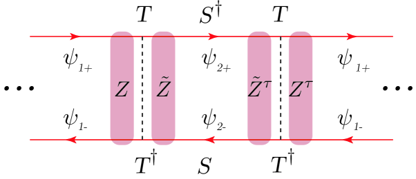
Figure 2: On the physical interpretation of the color-flavor transformation. Explanation, see text.

We apply the color-flavor transformation $B$ times – once for each phase $\phi_{b}$. As a result, we obtain a $B$–fold integral over supermatrices $Z_{b}$. There are four flavors (direction index $d=\pm 1$ and time-reversal index $t=1,2$). We combine all matrices $Z_{b}$ ($\tilde{Z}_{b}$) into a single block–diagonal $8B$-dimensional supermatrix $Z$ ($\tilde{Z}$) such that

$$Z_{bdts,b^{\prime}d^{\prime}t^{\prime}s^{\prime}}=\delta_{b,b^{\prime}}Z_{b\,dts,d^{\prime}t^{\prime}s^{\prime}}.$$ (43)

The averaged generating function now has the form

$$\begin{split}\langle\zeta(j_{+},j_{-};s)\rangle=&\mathrm{sdet}(T_{+}T_{-}^{\dagger})^{2}\int d(\tilde{\psi},\psi)\int d(\tilde{Z},Z)\\ &\mathrm{sdet}(1-\tilde{Z}Z)\,e^{-\bm{S}(\tilde{\Psi},\Psi,\tilde{Z},Z)}\end{split}$$ (44)

where

$$\begin{split}\bm{S}(\tilde{\Psi},\Psi,\tilde{Z},Z)=&\tilde{\Psi}_{1}\begin{pmatrix}\mathbbm{1}&Z\\ Z^{\tau}&\mathbbm{1}\end{pmatrix}\Psi_{1}+\\ &\tilde{\Psi}_{2}\begin{pmatrix}\mathcal{S}_{+}^{\dagger}&\tilde{Z}^{\tau}\\ \tilde{Z}&\mathcal{S}_{-}\end{pmatrix}\Psi_{2},\end{split}$$ (45)

and we used $2\tilde{\Psi}_{1}Z\Psi_{1}=\tilde{\Psi}_{1}Z\Psi_{1}+\tilde{\Psi}_{1}Z^{\tau}\Psi_{1}$, $2\tilde{\Psi}_{2}\tilde{Z}\Psi_{2}=\tilde{\Psi}_{2}\tilde{Z}\Psi_{2}+\tilde{\Psi}_{2}\tilde{Z}^{\tau}\Psi_{2}$. Here, the indices $1$, $2$ refer to the auxiliary index $x$, and the matrix structure is in advanced/retarded space. Integrating the Gaussian fields $\tilde{\Psi}$ and $\Psi$ we arrive at the (exact) representation

$$\langle\zeta(j_{+},j_{-};s)\rangle=\int d(\tilde{Z},Z)e^{-\bm{S}(\tilde{Z},Z)}$$ (46)

where the action is given by

$$\begin{split}\bm{S}(\tilde{Z},Z)=&-\mathrm{str}\,\mathrm{log}\,(1-\tilde{Z}Z)+\frac{1}{2}\mathrm{str}\,\mathrm{log}\,(1-Z^{\tau}Z)\\ &+\frac{1}{2}\mathrm{str}\,\mathrm{log}\,(1-\mathcal{S}_{+}\tilde{Z}^{\tau}\mathcal{S}_{-}^{\dagger}\tilde{Z}).\end{split}$$ (47)

(Note, that the prefactor $\mathrm{sdet}(T_{+}T_{-}^{\dagger})^{2}$ has canceled out.)

Before carrying on, let us pause to discuss the advantage gained by switching to the $Z$–representation. Consider the bilinears $\tilde{\psi}_{(+/-),s,x,d,b}e^{(+/-)i\phi_{b}}\psi_{(+/-),s,x,d,b}$ appearing as building blocks of the original phase–representation. Loosely identifying $\psi_{+/-}$ as retarded/advanced wave function amplitudes, these products describe the scattering of single particle states off phase fluctuations. Due to the effective randomness of the phases they fluctuate in a wild and non–controllable manner (see Fig. 2 for a cartoon of the propagation of a retarded [upper line] and advanced [lower line] wave function in space: a rapid succession of scattering events [the vertical dashed lines] leads to strong fluctuations.) Technically, this means that the original representation defies controlled evaluation schemes (such as mean field approximations and the like.)

In contradistinction, the $Z$–field enters the theory as $\sim\tilde{\Psi}_{+,s,t,d,b}Z_{b,ss^{\prime},tt^{\prime},dd^{\prime}}\Psi_{-,s^{\prime},t^{\prime},d^{\prime},b}$, i.e. through structures that couple retarded and advanced amplitudes locally in space. While (prior to the phase averaging) each of the $\Psi_{+/-}$ amplitudes individually was a rapidly fluctuating contribution, the product $\tilde{\Psi}_{+}\Psi_{-}$ contains benign, slowly fluctuating contributions. This is because the phase $\exp(i\phi)$ picked up by the retarded amplitude may cancel against the phase $\exp(-i\phi)$ carried by the advanced amplitude. In a semiclassical manner of speaking, this happens if the two amplitudes propagate along Feynman paths locally correlated in space. The advantage of the $Z$–representation is that it selects precisely these slowly fluctuating, spatially correlated bilinears which survive the averaging over phases. In Fig. 2, the $Z$–fields are indicated by vertical ovals. Wave function amplitudes qualifying to form a slowly fluctuating couple may carry different time–reversal and directional indices which explains the matrix–structure of $Z$ in these index spaces. At any rate, the structure of the color–flavor transformed theory indicates that the $Z$–integral will be comparatively benign and amenable to stationary phase treatment.

IV Saddle point analysis and universality

The action (36) provides for an exact representation of the generating functional of an individual graph. While the integral over $Z$ cannot be done in closed form, it turns out to be ideally suited to a mean field treatment. In the following, we will formulate the mean field analysis and explore under which conditions the theory reduces to one that predicts universal GOE statistics. (We assume time reversal invariance throughout.)

Our strategy will be to first identify uniform ’zero mode’ solutions to the mean field equations, and the corresponding mean field action. We will find that the integral over the reduced action generates an exact RMT expression for the spectral determinants. In a second step we proceed to investigate the validity of the zero mode approximation, i.e. we will explore under which conditions corrections to the RMT result vanish in the semiclassical limit $B\to\infty$.

IV.1 The zero-mode and universality

We begin by expanding the full action to linear order in the sources $p\pm=\Delta(\pm s-\sigma_{3}^{\mathbf{BF}}j_{\pm})$

$$\begin{split}\bm{S}(\tilde{Z},Z)=&\bm{S}_{0}(\tilde{Z},Z)\\ &-\frac{i}{4}\mathrm{str}\frac{p_{+}(\mathcal{L}\mathcal{S}+\mathcal{S}\mathcal{L})\tilde{Z}^{\tau}\mathcal{S}^{\dagger}\tilde{Z}}{1-\mathcal{S}\tilde{Z}^{\tau}\mathcal{S}^{\dagger}\tilde{Z}}\\ &+\frac{i}{4}\mathrm{str}\frac{p_{-}(\mathcal{L}\mathcal{S}^{\dagger}+\mathcal{S}^{\dagger}\mathcal{L})\tilde{Z}\mathcal{S}\tilde{Z}^{\tau}}{1-\mathcal{S}^{\dagger}\tilde{Z}\mathcal{S}\tilde{Z}^{\tau}}\\ &+\mathcal{O}\left((p\mathcal{L})^{2}\right)\end{split}$$ (48)

Here, $\bm{S}_{0}(Z,\tilde{Z})$ is obtained from (47) by replacing $\mathcal{S}_{\pm}\rightarrow\mathcal{S}$, and $\mathcal{L}_{bb^{\prime}}=\delta_{bb^{\prime}}L_{b}$ contains the bond length on its diagonal. Since we are only interested in spectral fluctuations on the scale of the mean level spacing $p_{\pm}\sim\mathcal{O}(B^{-1})$ implying that higher orders in the expansion in $p_{\pm}$ vanish in the limit $B\rightarrow\infty$. At this point we have to assume moderate bond length fluctuations such that $L_{b}/\overline{L}\ll B$.

To identify the mean field configurations of the theory, we differentiate the action $\bm{S}_{0}$ w.r.t. $Z$ and obtain

$$\frac{1}{1-\tilde{Z}Z}\tilde{Z}-\frac{1}{1-Z^{\tau}Z}Z^{\tau}=0$$ (49)

This equation is solved by

$$Z=\tilde{Z}^{\tau}.$$ (50)

Differentiating w.r.t. $\tilde{Z}$ and using (50) a second saddle–point equation assumes the form

$$\begin{split}\frac{1}{1-Z\tilde{Z}}Z-\frac{1}{2}\frac{1}{1-\mathcal{S}Z\mathcal{S}^{\dagger}\tilde{Z}}\mathcal{S}Z\mathcal{S}^{\dagger}-&\\ \frac{1}{2}\frac{1}{1-\mathcal{S}^{\tau}Z\mathcal{S}^{\dagger\tau}\tilde{Z}}\mathcal{S}^{\tau}Z\mathcal{S}^{\dagger\tau}&=0.\end{split}$$ (51)

This equation is solved by all field configurations that commute with the scattering operators, i.e.

$$\begin{split}Z_{0b,dts,d^{\prime}t^{\prime}s^{\prime}}=&\delta_{dd^{\prime}}Y_{ts,t^{\prime}s^{\prime}}\\ \tilde{Z}_{0b,dts,d^{\prime}t^{\prime}s^{\prime}}=&\delta_{dd^{\prime}}\tilde{Y}_{ts,t^{\prime}s^{\prime}},\end{split}$$ (52)

which corresponds to equidistribution on the set of directed bonds. The symmetry condition $\tilde{Z}=Z^{\tau}$ obtained from the first saddle–point equation implies $\tilde{Y}=Y^{\tau}$ where $Y^{\tau}=\tau_{0}Y^{T}\tau_{0}^{-1}$ and the matrix $\tau_{0}$ has been defined in (31). The commuting parts of these matrices obey $\tilde{Y}_{\mathbf{bb}}=Y^{*}_{\mathbf{bb}}$ and $\tilde{Y}_{\mathbf{ff}}=-Y^{*}_{\mathbf{ff}}$ while the non–commuting entries are all independent integration variables. The fermion-fermion part is integrated over $\mathbbm{R}^{4}\simeq\mathbbm{C}^{2}$ while boson-boson part is restricted to the compact region where all eigenvalues of $Y_{\mathbf{bb}}^{\dagger}Y_{\mathbf{bb}}$ are less than unity.

Reducing the action (48) to the zero-mode the first contribution vanishes exactly $\bm{S}_{0}(Z_{0},\tilde{Z}_{0})=0$ while the remaining term becomes

$$\bm{S}^{\mathrm{GOE}}(\tilde{Y},Y)=+i\frac{\pi}{\Delta}\mathrm{str}\frac{p_{+}Y\tilde{Y}}{1-Y\tilde{Y}}-i\frac{\pi}{\Delta}\mathrm{str}\frac{p_{-}\tilde{Y}Y}{1-\tilde{Y}Y},$$ (53)

Restricting the integration to the zero mode sector, we obtain

$$\langle\zeta(j_{+},j_{-};s)\rangle\simeq\zeta^{\mathrm{GOE}}(j_{+},j_{-};s)\rangle\equiv\int d(\tilde{Y},Y)e^{-\bm{S}^{\mathrm{GOE}}(Y,\tilde{Y})},$$ (54)

where the denotation $\zeta^{\mathrm{GOE}}$ indicates that the matrix integral over $Y$ obtains but an exact representation of the GOE correlation function. To represent the integral on the r.h.s. in a more widely recognizable form, let us define the $8\times 8$ supermatrix

$$\begin{split}Q=&\begin{pmatrix}\mathbbm{1}&Y\\ \tilde{Y}&\mathbbm{1}\end{pmatrix}\Sigma_{z}\begin{pmatrix}\mathbbm{1}&Y\\ \tilde{Y}&\mathbbm{1}\end{pmatrix}^{-1}\\ =&\begin{pmatrix}1+2Y\tilde{Y}/(1-Y\tilde{Y})&-2Y/(1-\tilde{Y}Y)\\ 2\tilde{Y}/(1-Y\tilde{Y})&-1-2\tilde{Y}Y/(1-\tilde{Y}Y)\end{pmatrix},\end{split}$$ (55)

where $\Sigma_{z}=\left(\begin{smallmatrix}\mathbbm{1}&0\\ 0&-\mathbbm{1}\end{smallmatrix}\right)$. It is then a straightforward matter to show that the action $\bm{S}(\tilde{Y},Y)$ takes the form of Efetov’s action Efetov for the GOE correlation function

$$\zeta^{\mathrm{GOE}}(j_{+},j_{-};s)=\int dQ\,e^{i\bm{S}(Q)}$$ (56)

where the measure is given by $dQ\equiv d(\tilde{Y},Y)$,

$$\bm{S}(Q)=\frac{\pi}{2}\mathrm{str}\,(Q-\Sigma_{z})\hat{\epsilon}$$ (57)

and $\hat{\epsilon}=-\frac{1}{\Delta}\left(\begin{smallmatrix}p_{+}&0\\ 0&p_{-}\end{smallmatrix}\right)$. For a discussion of the integral (56), and the ways random matrix predictions are obtained by integration over $Q$, we refer to the textbook Efetov .

IV.2 Validity of the saddle–point approximation

In the previous section we have shown that the reduction of the theory to a zero mode integral obtains GOE spectral correlations. However, we have not yet shown under which conditions this reduction is actually legitimate. This is the question to which we turn next.

For the purposes of our discussion, it will be sufficient to consider the expansion of the exact action (48) to second order in the fields $Z$,

$$\begin{split}\bm{S}^{(2)}(Z,\tilde{Z})=&\bm{S}_{0}^{(2)}(Z,\tilde{Z})\\ &-\frac{i}{4}\mathrm{str}\left(p_{+}(\mathcal{L}\mathcal{S}+\mathcal{S}\mathcal{L})\tilde{Z}^{\tau}\mathcal{S}^{\dagger}\tilde{Z}\right)\\ &+\frac{i}{4}\mathrm{str}\left(p_{-}(\mathcal{L}\mathcal{S}^{\dagger}+\mathcal{S}^{\dagger}\mathcal{L})\tilde{Z}\mathcal{S}\tilde{Z}^{\tau}\right),\end{split}$$ (58)

where

$$\bm{S}_{0}^{(2)}(Z,\tilde{Z})=\mathrm{str}\left(\tilde{Z}Z-\frac{1}{2}Z^{\tau}Z-\frac{1}{2}\mathcal{S}_{-}^{\dagger}\tilde{Z}\mathcal{S}_{+}\tilde{Z}^{\tau}\right).$$ (59)

Physically, the quadratic action describes the joint propagation of a retarded and an advanced Feynman amplitude along the same path in configuration space. (This is a generic feature of second order expansions to nonlinear $\sigma$–models of disordered and chaotic systems. For a discussion of this point, we refer to Ref. Efetov .) It thus carries information similar to that obtained from the diagonal approximation to semiclassics. The second order expansion is justified if the fluctuations of the fields $Z$ are massively damped (in the sense that the matrix elements of $Z$ effectively contributing to the integral are much smaller than unity.) Under these conditions, the integration over matrix elements of $Z$ may be extended to infinity and we obtain a genuine Gaussian integral.

The eigenvalues of the quadratic form appearing in $\bm{S}^{(2)}$ at $p_{\pm}=0$ determine the damping $m_{j}$ — or the mass, in a field theoretical jargon — inhibiting fluctuations of the eigenmodes $Z_{j}$. As indicated by its name, the zero–mode $Z_{0}$ carries zero mass. Within the quadratic approximation, the correlation function assumes the form $\langle\zeta(J_{+},j_{-};s)\rangle\simeq\langle\zeta(J_{+},j_{-};s)\rangle^{(2)}=\prod_{j}I_{j}$, with the Gaussian integrals

$$\begin{split}I_{j}=\int d(Z_{j},\tilde{Z}_{j})&\exp[-\mathrm{str}\{m_{j}Z_{j}\tilde{Z}_{j}\\ &+i(m-1)\overline{L}(p_{+}Z_{j}\tilde{Z}_{j}-p_{-}\tilde{Z}_{j}Z_{j})\}]\end{split}$$ (60)

where $Z_{j}$, and $\tilde{Z}_{j}$ are $4\times 4$ supermatrices obeying the ubiquitous condition $\tilde{Z}_{j\mathbf{bb}}=Z^{*}_{j\mathbf{bb}}$ and $\tilde{Z}_{j\mathbf{ff}}=-Z^{*}_{j\mathbf{ff}}$. We also assumed here, that the first saddle–point equation $Z=\tilde{Z}^{\tau}$ is obeyed which reduces the number of integration variables by a factor $1/2$. Configurations which are orthogonal to this condition give the same kind of factors but have different masses. Doing the Gaussian integral Gaussian we obtain

$$I_{m}=\frac{[1+i\frac{\pi(m-1)(s+j_{\Sigma})}{mB}]^{2}[1+i\frac{\pi(m-1)(s-j_{\Sigma})}{mB}]^{2}}{[1+i\frac{\pi(m-1)(s+j_{\Delta})}{mB}]^{2}[1+i\frac{\pi(m-1)(s-j_{\Delta})}{mB}]^{2}},$$ (61)

where $j_{\Delta}=j_{+}-j_{-}$ and $j_{\Sigma}=j_{+}+j_{-}$. Differentiating w.r.t. the sources we finally obtain the quadratic approximation to the correlation function,

$$\begin{split}R^{(2)}_{2}(s)=&\sum_{m}\frac{1}{8\pi^{2}}\mathrm{Re}\,\frac{\partial^{2}}{\partial j_{+}\partial j_{-}}I_{m}\big{|}_{j_{\pm}=0}\\ =&\sum_{m}\frac{(m-1)^{2}(m^{2}B^{2}-\pi^{2}(m-1)^{2}s^{2})}{(m^{2}B^{2}+\pi^{2}(m-1)^{2}s^{2})^{2}}.\end{split}$$ (62)

The contribution of the zero mode ($m=0$) is given by $-\frac{1}{\pi^{2}s^{2}}$ and coincides with the diagonal approximation to the GOE correlation function. (Later on we shall see that in the case of broken time reversal invariance, one half of the matrix elements of $Z_{0}$ become massive implying that the contribution of the zero mode reduces to the GUE expression $-\frac{1}{2\pi^{2}s^{2}}$.)

In the limit $B\to\infty$, the $s$-dependence of the contribution of massive modes to the correlation function is negligible for our purpose, i.e. individual modes contribute maximally as $\sim(m-1)^{2}/2m^{2}B^{2}\sim(mB)^{-2}$. Only modes of mass $m\sim B^{-\alpha}$, where $\alpha$ is a non–vanishing positive exponent, can survive the limit $B\to\infty$. The contribution of an individual mode is negligible if the exponent $0\leq\alpha<1$. There are at most $\mathcal{O}(B)$ nearly massless modes, and we are led to require that $B^{2\alpha-1}$ must vanish in the limit of large graphs $B\rightarrow\infty$, or that $0\leq\alpha<1/2$.

After these general remarks, let us discuss the masses that actually appear in the quadratic action (59). We first show that modes violating the first saddle–point equation $Z=\tilde{Z}^{\tau}$ can safely be neglected. This is seen by rewriting the quadratic action as $\bm{S}^{(2)}=\frac{1}{2}\mathrm{str}\left[(Z-\tilde{Z}^{\tau})(\tilde{Z}-Z^{\tau})+\tilde{Z}^{\tau}\tilde{Z}-\mathcal{S}_{+}\tilde{Z}^{\tau}\mathcal{S}_{-}^{\dagger}\tilde{Z}\right]$. This expression shows that fluctuations away from the condition $Z=\tilde{Z}^{\tau}$ are suppressed by a large mass of $\mathcal{O}(1)$. These fluctuations may safely be ignored, i.e. we may assume the condition $Z=\tilde{Z}^{\tau}$ to be rigidly imposed. The quadratic action then assumes the reduced form

$$\bm{S}^{(2)}(Z)=\frac{1}{2}\mathrm{str}\left[Z\tilde{Z}-\mathcal{S}_{+}Z\mathcal{S}_{-}^{\dagger}\tilde{Z}\right]$$ (63)

where the condition $Z=\tilde{Z}^{\tau}$ reduces the number of independent integration variables by a factor one half.

We next show that fluctuations $Z_{d,d^{\prime}},d\not=d^{\prime}$ off–diagonal in the directional indices may safely be discarded, too. To this end, let us separate the contribution of diagonal and off–diagonal fields, $Z^{\rm diag}$ and $Z^{\rm off}$, respectively, to the quadratic action (63):

$$\mathrm{str}(\mathcal{S}Z\mathcal{S}^{\dagger}\tilde{Z})=\mathrm{str}\begin{pmatrix}\tilde{Z}^{\mathrm{diag}}&\tilde{Z}^{\mathrm{off}}\end{pmatrix}\begin{pmatrix}\mathcal{F}&\mathcal{G}\\ \mathcal{H}&\mathcal{K}\end{pmatrix}\begin{pmatrix}Z^{\mathrm{diag}}\\ Z^{\mathrm{off}}\end{pmatrix}.$$ (64)

The matrices $\mathcal{G}$ and $\mathcal{H}$ contain elements of the type $S_{b\,-d,b^{\prime}d^{\prime}}S^{*}_{bd,b^{\prime}d^{\prime}}$ or $S_{b^{\prime}\,-d^{\prime},bd}S^{*}_{bd,b^{\prime}d^{\prime}}$. If $S^{*}_{bd,b^{\prime}d^{\prime}}$ does not vanish there must be a vertex $v$ in the graph, such that the directed bond $(b^{\prime},d^{\prime})$ ends at $v$ and $(b,d)$ starts at $v$. The partner factors $S_{b\,-d,b^{\prime}d^{\prime}}$ and $S_{b^{\prime}\,-d^{\prime},bd}$ then vanish (unless the bond $b$ is a loop such that $(b,d)$ and $(b,-d)$ both start and end at the vertex $v$. However, for simple graphs no loops are present and $\mathcal{G}=\mathcal{H}=0$.) The matrix $\mathcal{K}$ contains elements of the form $S_{b\,-d,b^{\prime}\,-d^{\prime}}S^{*}_{bd,b^{\prime}d^{\prime}}$ or $S_{b^{\prime}d^{\prime},bd}S^{*}_{bd,b^{\prime}d^{\prime}}$. For $b\not=b^{\prime}$, these vanish (unless the bonds $b$ and $b^{\prime}$ connect the same pair of vertices which, however, is forbidden for simple graphs.) For $b=b^{\prime}$, the non–vanishing of the matrix element would again require the existence of loops. We thus conclude that $\mathcal{K}=0$. Decoupled from the scattering operators, the integration over modes $Z_{d\not=d^{\prime}}$ merely produces a factor of unity (supersymmetry!) so that we will concentrate on the complementary set of modes

$$\begin{split}Z_{b\,dd^{\prime}}&=\delta_{dd^{\prime}}Z_{bd}\\ \tilde{Z}_{b\,dd^{\prime}}&=\delta_{dd^{\prime}}\tilde{Z}_{bd},\end{split}$$ (65)

throughout. The contribution of these configurations to the generating function is determined by the elements of the matrix $\mathcal{F}=\{|S_{bd,b^{\prime}d^{\prime}}|^{2}\}$. (Here, we used that for a time reversal invariant graph, $|S_{bd,b^{\prime}d^{\prime}}|^{2}=S_{bd,b^{\prime}d^{\prime}}S_{b^{\prime}\,-d^{\prime},b\,-d}^{*}$, i.e. that the matrix $\mathcal{F}$ is isotropic in time reversal space.) Specifically, the action ${\bf S}_{0}$ assumes the form

$$\bm{S}^{(2)}={1\over 2}\mathrm{str}(\tilde{Z}(\mathbbm{1}-\mathcal{F})Z)$$ (66)

Within the context of the semiclassical analysis of appendix A, we have seen that the matrix $\mathcal{F}$ determines the classical propagator (the Frobenius–Perron operator) on the graph. Comparing with our discussion above, we conclude that the eigenvalues of that operator, $\lambda_{i}$, determine the ‘mass spectrum’ $\{m_{i}=1-\lambda_{i}\}$ of the theory. We have seen that large graphs behave universal if the masses scale as $m_{i}\sim B^{-\alpha}$, $0\leq\alpha<1/2$. Specifically, this condition requires the gap $1-\lambda_{1}$ between the zeroth Perron–Frobenius eigenvalue $\lambda_{0}=1$ (corresponding to the fully equilibrated zero–mode configuration) and the first ‘excited’ state to scale as $1-\lambda_{1}\equiv\Delta_{g}\gtrsim B^{-\alpha},0\leq\alpha<1/2$. This condition is stricter then Tanners conjecture $0\leq\alpha<1$: For $\alpha\geq 1$, corrections to the universal result remain sizeable no matter how large the graph is. In the intermediate region $1/2\leq\alpha<1$ — permissible by Tanner’s criterion — non–universal corrections vanish only if the number $r$ of classical modes with a small mass remains constant (or does not grow too fast) such that $B^{2}\Delta_{g}^{2}/r\rightarrow\infty$. If, however, the number of low energy modes is extensive, $r\sim B$, the stricter condition $0\leq\alpha<1/2$ has to be imposed to stabilize universality.

Above we have shown that in the limit $B\to\infty$ only the zero mode effectively contributes to the correlation function (provided, of course, the master condition $\Delta_{g}\sim B^{-\alpha}$ is met.) While the zero mode integral must be performed rigorously, all other modes are strongly overdamped and may be treated in a quadratic approximation. (This is the a posteriori justification for the quadratic approximation on which our analysis of the mass spectrum was based.)

IV.3 GOE-GUE crossover

The analysis above applied to time reversal invariant graphs. In this section we discuss what happens if time reversal invariance gets gradually broken, e.g. by application of an external magnetic field. We assume full universality, i.e. $B\Delta_{g}^{2}\gg 1$ such that only the zero–mode contributes to $R_{2}(s)$. Our aim is to derive a condition for the crossover between GOE–statistics (time reversal invariance) and GUE–statistics (lack of time reversal invariance.)

The substructure of the $Z$–fields in time reversal space is given by

$$Z_{b}=\begin{pmatrix}Z_{\mathbf{D},b}&Z_{\mathbf{C,b}}\\ \tilde{Z}_{\mathbf{C},b}^{T}\sigma_{3}^{\mathbf{BF}}&\tilde{Z}_{\mathbf{D},b}^{T}\end{pmatrix},\qquad\tilde{Z}_{b}=\begin{pmatrix}\tilde{Z}_{\mathbf{D},b}&\sigma_{3}^{\mathbf{BF}}Z_{\mathbf{C},b}^{T}\\ \tilde{Z}_{\mathbf{C},b}&Z_{\mathbf{D},b}^{T}\end{pmatrix},$$ (67)

where $Z_{\mathbf{D/C},b}$ and $\tilde{Z}_{\mathbf{D/C},b}$ are $2\times 2$ supermatrices subject to the constraint $\tilde{Z}_{\mathbf{bb}}=Z^{*}_{\mathbf{bb}}$ and $\tilde{Z}_{\mathbf{ff}}=-Z^{*}_{\mathbf{ff}}$, while the non–commuting entries of these matrices are independent integration variables. The subscripts $\mathbf{D}(\mathbf{C})$ allude to the fact that in disordered fermion systems, the modes $Z_{\mathbf{D}}$ ($Z_{\mathbf{C}}$) generate the so–called diffuson (Cooperon) excitations. Physically, the former (latter) describe the interference of two states as they propagate along the same path (the same path yet in opposite direction) in configuration space; Cooperon modes are susceptible to time reversal invariant breaking perturbations.

Substituting this representation into the quadratic action, we obtain

$$\bm{S}^{(2)}=\mathrm{str}\left(\tilde{Z}_{\mathbf{D}}(\mathbbm{1}-\mathcal{F}_{\mathbf{D}})Z_{\mathbf{D}}+\tilde{Z}_{\mathbf{C}}(\mathbbm{1}-\mathcal{F}_{\mathbf{C}})Z_{\mathbf{C}}\right)$$ (68)

as a generalization of Eq. (66). Here, $\mathcal{F}_{\mathbf{D}}=\{|S_{bd,b^{\prime}d^{\prime}}|^{2}\}$ while $\mathcal{F}_{\mathbf{C}}=S_{bd,b^{\prime}d^{\prime}}S_{b^{\prime}\,-d^{\prime},b\,-d}^{*}$. For a time reversal non–invariant graph $\mathcal{F}_{\mathbf{D}}\not=\mathcal{F}_{\mathbf{C}}$ and the symmetry of the action in time reversal invariance space gets lost.

Noting that $2B=\sum_{bd,b^{\prime}d^{\prime}}|S_{bd,b^{\prime}d^{\prime}}|^{2}$, we conclude that the Cooperon zero mode $Z_{\mathbf{C},b}=Y_{\mathbf{C}}$ acquires a mass term $\sim Bm_{\mathbf{C}}\,\mathrm{str}(Y_{\mathbf{C}}\tilde{Y}_{\mathbf{C}})$, where the coefficient

$$\begin{split}m_{\mathbf{C}}&=\frac{1}{2B}\left|\sum_{bd,b^{\prime}d^{\prime}}S_{bd,b^{\prime}d^{\prime}}(S^{*}_{bd,b^{\prime}d^{\prime}}-S^{*}_{b^{\prime}d^{\prime-1},bd^{-1}})\right|\\ &=\frac{1}{B}\left|\mathrm{tr}\,S^{\dagger}(S-\sigma_{1}^{\mathrm{dir}}S^{T}\sigma_{1}^{\mathrm{dir}})\right|\end{split}$$ (69)

measures the degree of the breaking of the symmetry $S=S^{\mathcal{T}}$. The Cooperon mode may be neglected once $Bm_{\mathbf{C}}\rightarrow\infty$ as $B\rightarrow\infty$.

For the sake of definiteness, let us discuss two concrete mechanisms of symmetry breaking: i. breaking the time–reversal symmetry of vertex scattering matrices, and ii. application a magnetic field.

Beginning with i., let us consider a large complete graph for simplicity. (A graph is complete if any two of its vertices are connected by a bond.) The number of vertices of these graphs is order $B^{1/2}$, and each column in $S_{b^{\prime}d^{\prime},bd}$ has $B^{1/2}$ non–vanishing entries of order $B^{-1/4}$. Breaking time–reversal symmetry at a single vertex thus results in a coefficient $m_{\mathbf{C}}\sim B^{-1}$. Breaking time–reversal invariance at a single vertex is, thus, not sufficient to drive the crossover to GUE statistics. Rather, a finite fraction $\sim B^{\beta}$ ($\beta>0$) of time–reversal non–invariant vertices is required. Obtained for the simple case of complete graphs, it is evident that this conclusion generalizes to generic graphs.

Turning to ii., the application of a constant magnetic field $A_{b}=A$ causes a global change of all its bond scattering matrices; We have to replace $T(k)=e^{ik\mathcal{L}/2}\rightarrow T(k)T(\sigma_{3}^{\mathbf{dir}}A)=e^{i(k+\sigma_{3}^{\mathbf{dir}}A)\mathcal{L}/2}$. This is equivalent to replacing $S\rightarrow S(A)=T(\sigma_{3}^{\mathbf{dir}}A)ST(\sigma_{3}^{\mathbf{dir}}A)$ in the quantum map. Assuming time–reversal invariance at $A=0$ the mass of the cooperon mode becomes

$$\begin{split}m_{\mathbf{C}}(A)&=\frac{1}{2B}\left|\mathrm{tr}\,S^{\dagger}[S-T(-\sigma_{3}^{\mathbf{dir}}A)ST(-\sigma_{3}^{\mathbf{dir}}A)]\right|\\ &\approx A^{2}\mu_{2}+\mathcal{O}(A^{3})\end{split}$$ (70)

where we used $\sigma_{1}\sigma_{3}\sigma_{1}=-\sigma_{3}$. We may estimate

$$\mu_{2}\approx\frac{\overline{L}}{4B}\left|\mathrm{tr}\,\left(S^{\dagger}\sigma_{3}^{\mathbf{dir}}S\sigma_{3}^{\mathbf{dir}}-1\right)\right|$$ (71)

by setting $T(-\sigma_{3}^{\mathbf{dir}}A)\approx e^{-i\frac{A\overline{L}}{2}\sigma_{3}^{\mathbf{dir}}}$. For a generic scattering matrix one may expect $|\mathrm{tr}\,\left(S^{\dagger}\sigma_{3}^{\mathbf{dir}}S\sigma_{3}^{\mathbf{dir}}-1\right)|\sim B$ such that a small magnetic field of order $A\sim B^{-1/2}$ is strong enough to induce the crossover to GUE statistics. (Assuming that the geometric ‘area’ of the graph, $S\sim B$, is proportional to the number of bonds, we conclude that the crossover takes place once a finite number $\sim AS\times e/h\sim B^{0}$ of flux quanta pierces the system. This crossover criterion is known to apply quite generically in disordered or chaotic quantum systems.)

V Conclusion

To summarize, we have shown that the two–point spectral correlation function of individual quantum graphs coincides with the prediction of random–matrix theory. Corrections to universality vanish in the limit $B\rightarrow\infty$ provided the gap in the spectrum of the underlying ‘classical’ propagator remains constant, or vanishes as $|m|=|1-\lambda_{2}|\sim B^{-\alpha}$ with $0\leq\alpha<1/2$. These results were obtained by representing the generating functional of the two–point correlation function in terms of a nonlinear $\sigma$–model. Closely resembling the theory of spectral correlations in disordered fermion systems, this formalism obtained a fairly accurate picture of correlations in the graph spectrum. Specifically, (i) a perturbative expansion of the $\sigma$–model for large energies establishes the contact with semiclassical approaches to the problem, (ii) for low energies a non–perturbative integration over the fully phase–space equilibrated zero mode configuration of the model obtains spectral correlations as predicted by random matrix theory, and (iii) the analysis of the ‘mass spectrum’ of non–uniform modes yields conditions under which universality is to be expected: In the limit of large graph size, $B\to\infty$, the first non–vanishing eigenvalue of the classical Perron–Frobenius operator on the graph must be separated from unity by scale $\Delta_{g}$ larger than $\mathrm{const.}\times B^{-\alpha}$, $0\leq\alpha<1/2$.

This condition turns out to be met by many prominent classes of quantum graphs. Examples include complete DFT graphs, or complete Neumann graphs greg . It has also been shown that almost all unistochastic matrices, i.e. matrices of the type $\mathcal{F}_{ij}=|S_{ij}|^{2}$, where $S$ runs over the unitary group (or, equivalently the circular unitary ensemble CUE), have a finite gap in the limit of large matrices gregongap . For example, star graphs stars with the central vertex scattering matrix $S_{ij}$ generically display universal spectral statistics. (Counterexamples such as the Neumann star graph gregonstars are not generic in this sense.)

Cases where the universality condition is violated include large graphs with low valency (coordination number) of vertices. In such systems Anderson localization phenomena may interfere with the buildup of universal correlationsschanz ; solomyak .

Appendix A Periodic orbit theory for graphs and Tanner’s conjecture

For completeness we briefly review some elements of the periodic orbit approach to spectral statistics on quantum graphs. Central to the periodic orbit approach is a short-time expansion of the spectral form factor, $K(\tau)$, the Fourier transform of the two–point correlation function $R_{2}(s)=\int_{0}^{\infty}K(\tau)e^{i2\pi s\tau}$. For moderate bond length fluctuations in quantum graphs this quantity is usually replaced by the essentially equivalent quantity

$$K_{n}=\frac{1}{2B}\left\langle\mathrm{tr}\,\mathcal{U}_{B}(k)^{n}\mathrm{tr}\,{\mathcal{U}_{B}(k)^{\dagger}}^{n}\right\rangle_{k}.$$ (72)

Here $n\in\mathbbm{N}$ is a discrete time corresponding to $\tau={n}{2B}$. This discrete version of the form factor is connected to the correlations in the eigenphases of the quantum map.

The form factor (72) is a double sum over periodic orbits $\gamma,\gamma^{\prime}$ of lengths $n$ where a periodic orbit on the graph is a periodic sequence of directed bonds visited. In the diagonal approximation — valid for short times $n\ll 2B$ — only those pairs of orbits are taken into account where $\gamma^{\prime}=\gamma$, or $\gamma^{\prime}=\gamma^{T}$ where $\gamma^{T}$ is the time-reversed periodic orbit:

$$K_{n}^{\mathrm{diag}}=\frac{n}{B}\mathrm{tr}\,F^{n}$$ (73)

where

$$F_{bd,b^{\prime}d^{\prime}}=|S_{bd,b^{\prime}d^{\prime}}|^{2}$$ (74)

is the ’classical’ propability to be scattered from the directed bond $(b^{\prime},d^{\prime})$ to $(b,d)$. It can be considered as the equivalent of the Frobenius–Perron propagator for Hamiltonian flows. Due to unitarity of $S$ the matrix $F$ is bistochastic $\sum_{bd}F_{bd,b^{\prime}d^{\prime}}=\sum_{bd}F_{b^{\prime}d^{\prime},bd}=1$ and describes a Markov process on the directed bonds of the graph. The eigenvalues $\lambda_{i}$ of bistochastic matrices are known to lie in the unit circle $|\lambda_{i}|\leq 1$ with at least one eigenvalue unity (here corresponding to equidistribution on the directed bonds.)

Universal spectral statistics is expected for ‘chaotic’ graphs in the limit $B\rightarrow\infty$. According to Eq. (73), the necessary condition for universality is given by

$$\mathrm{tr}\,F^{\tau 2B}\rightarrow 1,$$ (75)

where the scaled time $\tau\equiv n/2B\ll 1$ is kept constant and the limit $B\to\infty$ is implied. In this case, $K^{\rm diag}\to 2\tau$ in agreement with the short time expansion $K^{\mathrm{GOE}}(\tau)\stackrel{{\scriptstyle\tau\ll 1}}{{\simeq}}2\tau$ of the RMT–form factor

$$K^{\mathrm{GOE}}(\tau)=\begin{cases}|\tau|\left(2-\log(2|\tau|+1)\right)&\text{for $|\tau|<1$}\\ 2-|\tau|\log\frac{2|\tau|+1}{2|\tau|-1}&\text{for $|\tau|\geq 1$}.\end{cases}$$

Here, $\tau\equiv t\Delta/2\pi$ is time measured in units of the RMT–level spacing.

The universality condition above states that any propability distribution on the graph will eventually decay to equidistribution – a Markov process with this property is called ‘mixing’ which implies ergodicity (equality of long time-averages to an an average over the equidistribution on bonds). This is very week condition on a connected graph: a non-ergodic Markov map on a graph implies equivalence to a Markov map on a disconnected graph. However, as observed by Tanner Tanner the condition (75) is actually stronger than mixing dynamics (for an example of a mixing graph with non–universal spectral statistics — the Neumann star graph, see gregonstars ). This can be seen by rewriting the (75) in terms of the $2B$ eigenvalues $\lambda_{i}$ of $F$. Ordering the eigenvalues in magnitude such that $1=\lambda_{1}\geq|\lambda_{2}|\geq\dots$ and defining the spectral gap

$$\Delta_{\mathrm{gap}}=1-|\lambda_{2}|,$$ (76)

mixing dynamics merely implies $\Delta_{\mathrm{gap}}>0$, i.e. that $\lambda_{1}=1$ is the only eigenvalue on the unit circle. However, there are examples of graphs whose ‘classical’ dynamics is mixing while the form factor does not start as $2\tau$. To understand the origin of this exceptional behavior, notice that

$$\mathrm{tr}\,F^{n}=\sum_{i=1}^{2B}\lambda_{i}^{n}=1+\sum_{i=2}^{2B}\lambda_{i}^{n},$$ (77)

implying the universality criterion $|\sum_{i=2}^{2B}\lambda_{i}^{n}|\rightarrow 0$. With $|\sum_{i=2}^{2B}\lambda_{i}^{2B\tau}|\leq\sum_{i=2}^{2B}|\lambda_{i}|^{2B\tau}\leq(2B-1)(1-\Delta_{\mathrm{gap}})^{2B\tau}$. If $\Delta_{\mathrm{gap}}$ remains a finite constant as $B\rightarrow\infty$ this surely vanishes and universality is guaranteed. However if $\Delta_{\mathrm{gap}}=cB^{-\alpha}$ the correction to unity vanished only if $0\leq\alpha<1$. In all known examples of graphs where the spectral statistics is non–universal in spite of ergodic classical dynamics this condition is, indeed, violated: $\alpha\geq 1$. For this reason Tanner conjectured that $0\leq\alpha<1$ is a sufficient universality criterion in the scaling limit $\tau$ fixed while $B\rightarrow\infty$.

Appendix B Time–reversal invariant graphs with spin

In this appendix we discuss the spectral statistics of time–reversal invariant graphs with spin (symmetry class $A$II, or symplectic symmetry.) This case has been considered in connection with the Dirac equation on graphs Harrison . Following a somewhat different approach, we will here break spin rotational invariance by choosing vertex boundary conditions that couple different spin components (yet leave time–reversal invariance intact.)

A spin degree of freedom is straightforwardly introduced by adding a spin component $m=\pm\frac{1}{2}$ to the wave function on the bonds. This extension turns the quantum evolution map $\mathcal{U}_{B}(k)=T(k)ST(k)$ into a $4B\times 4B$ matrix. We consider non–magnetic graphs ($A_{b}=0$) and assume independent propagation of the spin components on the bonds: $T(k)_{bdm,b^{\prime}d^{\prime}m^{\prime}}=\delta_{b,b^{\prime}}\delta_{d,d^{\prime}}\delta_{m,m^{\prime}}e^{ikL_{b}/2}$. Mixing of spins occurs at the vertex scattering centers. Comprising all vertex scattering matrices into a single unitary matrix $S$ (defined in analogy to spinless case discussed in the text) we obtain the condition

$$S=S^{\mathcal{T}}\equiv\sigma^{\mathbf{dir}}_{\mathrm{1}}\sigma^{\mathbf{spin}}_{\mathrm{2}}S^{T}\sigma^{\mathbf{spin}}_{\mathrm{2}}\sigma^{\mathbf{dir}}_{\mathrm{1}}$$ (78)

for time-reversal invariance where $\sigma^{\mathbf{spin}}_{\mathrm{2}}=i\left(\begin{smallmatrix}0&-\mathbbm{1}\\ \mathbbm{1}&0\end{smallmatrix}\right)$ is the Pauli matrix in spin indices $m$. The corresponding anti–unitary time–reversal operator obeys $\mathcal{T}^{2}=-\mathbbm{1}$ characteristic of symmetry class is $A$II.

Any system in class $A$II has a doubly degenerate spectrum due to Kramers’ degeneracy. By convention, each of the doubly degenerate eigenvalues is counted only once, i.e. the mean level spacing $\Delta=\pi/B\overline{L}$ as with spinless graphs. The oscillatory contribution to the density of states is given by $\delta d(k)=-\frac{1}{2\pi}\mathrm{Im}\,\frac{d}{dk}\mathrm{ln}\,\xi(k^{+}).$

In essence, the derivation of field theory representation of the generating function parallels the spinless case. However, the generalized transposition is now defined as

$$\begin{split}\tau=&-i\sigma_{1}^{\mathbf{dir}}\sigma_{2}^{\mathbf{spin}}\tau_{0}\\ \tau_{0}=&-iE_{\mathbf{b}}\sigma_{2}^{\mathbf{tr}}+E_{\mathbf{f}}\sigma_{1}^{\mathbf{tr}},\end{split}$$ (79)

such that $\tau^{T}=\tau^{-1}$ and $\tau^{2}=-\tau_{0}^{2}=\sigma_{3}^{\mathbf{BF}}$. The definition of $\tau_{0}$ reflects the different type of time–reversal symmetry. Second, the presence of a spin component implies that the matrices $Z_{b}$ and $\tilde{Z}_{b}$ — introduced by color flavor transformation as before — now have dimension $16\times 16$. These differences understood, (47) applies to graphs with spin.

The saddle–point conditions identify a zero–mode diagonal in directional, and in spin indices $Z_{0b\,dmts,d^{\prime}m^{\prime}t^{\prime}s^{\prime}}=\delta_{dd^{\prime}}\delta_{mm^{\prime}}Y_{ts,t^{\prime}s^{\prime}}$ ($\tilde{Z}_{0b\,dmts,d^{\prime}m^{\prime}t^{\prime}s^{\prime}}=\delta_{dd^{\prime}}\delta_{mm^{\prime}}Y_{ts,t^{\prime}s^{\prime}}$) with $\tilde{Y}=Y^{\tau}$ where $Y^{\tau}=\tau_{0}Y^{T}\tau_{0}^{-1}$. In an explicit way of writing, the time reversal structure of the $Z$–matrices (or, equivalently, the $Y$–matrices) is given by

$$\begin{split}Z=&\begin{pmatrix}Z_{\mathbf{D}}&Z_{\mathbf{C}}\\ -\tilde{Z}_{\mathbf{C}}^{T}\sigma_{3}^{\mathbf{BF}}&\tilde{Z}_{\mathbf{D}}^{T}\end{pmatrix}\\ \tilde{Z}=&\begin{pmatrix}\tilde{Z}_{\mathbf{D}}&-\sigma_{3}^{\mathbf{BF}}Z_{\mathbf{C}}^{T}\\ \tilde{Z}_{\mathbf{C}}&Z_{\mathbf{D}}^{T}\end{pmatrix},\end{split}$$ (80)

Projected onto the zero–mode sector, the action is given by

$$\bm{S}^{\mathrm{GSE}}(\tilde{Y},Y)=+i\frac{2\pi}{\Delta}\mathrm{str}\frac{p_{+}Y\tilde{Y}}{1-Y\tilde{Y}}-i\frac{2\pi}{\Delta}\mathrm{str}\frac{p_{-}\tilde{Y}Y}{1-\tilde{Y}Y}.$$ (81)

Except for a factor $2$ (which accounts for Kramers’ degeneracy) this expression equals the GOE action (53); the difference between the two cases is hidden in the symmetry $Y=\tilde{Y}^{\tau}$. As with the GOE case above, an integration over the matrices $Y$ Efetov obtains the correlation function of the GSE.

Sufficient conditions for the zero–mode reducibility can be derived as in the spinless case. Modes violating the symmetry condition $Z=\tilde{Z}^{\tau}$, and modes off-diagonal in direction space may be discarded. Similarly, modes off–diagonal in the spin index $m$ are massive and may be neglected, too. Therefore, the validity of the saddle–point reduction again relies on the discreteness of the eigenmode spectrum of the ‘classical’ propagator $\mathcal{F}_{bdm,b^{\prime}d^{\prime}m^{\prime}}=|S_{bdm,b^{\prime}d^{\prime}m^{\prime}}|^{2}$.

Appendix C Color–flavor transformation

In this appendix we sketch the main conceptual input entering the proof of the color–flavor transformation (41). (For a detailed exposure of the proof, we refer to Zirnbauer .) Central to our discussion will be a (super)–algebra of operators defined as

$$[c_{A},c_{A}^{\prime}]\equiv c_{A}\bar{c}_{A}^{\prime}-(-)^{|A||A^{\prime}|}\bar{c}_{A^{\prime}}c_{A}=\delta_{A,A},$$ (82)

where $A=(a,\alpha)$, the index $\alpha,\alpha^{\prime}$ keeps track of all flavor components of the theory (boson/fermion, time–reversal, directional, etc.), and $a,a^{\prime}=\pm$ distinguish between retarded and advanced indices. These operators act in an auxiliary Fock–space, whose vacuum state is defined by the condition

$$c_{+,\alpha}|0\rangle=\bar{c}_{-,\alpha}|0\rangle=0,\qquad\langle 0|\bar{c}_{+,\alpha}=\langle 0|c_{-,\alpha}=0.$$

We may, thus, think of the vacuum as a configuration where all $(+)$–states are empty, while all $(-)$–states are filled; Excitations are formed by creating $+$–particles and $(-)$–holes.

The above Fock space contains a sub–space defined by the condition that each state contains as many excited $(+)$–particles as $(-)$–holes. We call this space as the flavor–space. (Alternatively, we may characterize the flavor–space as the space of all excitations that can be reached from the vacuum state without changing the number of particles.) In essence, color–flavor transformation amounts to the construction of two different representations of a projector onto the flavor space.

Representation no. 1 is constructed as follows: a generic state in Fock space can be represented as a linear combination $|\Psi\rangle=\sum_{n_{+},n_{-}}|\Psi_{n_{+},n_{-}}\rangle$, where $|\Psi_{n_{+},n_{-}}\rangle$ contains $n_{+/-}$ particle/hole states. A projection onto the flavor state can now be trivially effected by mapping

$$|\Psi\rangle\mapsto{\cal P}^{I}|\Psi\rangle\equiv{1\over 2\pi}\int d\phi\,e^{i(n_{+}-n_{-})\phi}|\Psi_{n_{+},n_{-}}\rangle.$$

To construct representation no. 2 some more of preparatory work is necessary: Consider the Lie–supergroup ${\rm Gl}(2F,2F)$ (the group of $(4F)$–dimensional invertible supermatrices.) This group acts in Fock space by the representation ${\rm Gl}(2F,2F)\ni g\mapsto T_{g}\equiv\exp(\bar{c}_{A}\,\ln(g)_{A,A^{\prime}}\,c_{A^{\prime}})$, where $T_{g}$ acts as linear map in Fock space. (For the proof that the assignment $g\mapsto T_{g}$ meets all criteria required of a group representation, see Zirnbauer .)

One may show that the representation above is irreducible in flavor space. This implies that the entire space may be generated by the action of the group on a fixed reference state, the vacuum state, say. The set of ‘coherent states’ $|g\rangle\equiv T_{g}|\Omega\rangle$ will play a crucial role in the construction of the flavor space projector. To bring them into a maximally simple form, we first note that transformations generated by elements $h\equiv{\rm bdiag}(h_{+},h_{-})\in H$ of the sub–group $H$ of matrices block–diagonal in advanced/retarded space leave the vacuum invariant (up to a constant.) Using the defining commutator relations (82) it is indeed straightforward to verify that $T_{h}|\Omega\rangle=|\Omega\rangle\times{\rm sdet}(h_{-})^{-1}$. Thus, transformations $T_{h}$ do not change the vacuum in an ‘essential’ way and it is sufficient to consider the action of the coset space $G/H$ on $|\Omega\rangle$. A parameterization of individual cosets $gH\in G/H$ optimally adjusted to our application below reads as

$$g=\left(\begin{matrix}(1-Z\tilde{Z})^{-1/2}&Z(1-\tilde{Z}Z)^{-1/2}\cr\tilde{Z}(1-Z\tilde{Z})^{-1/2}&(1-\tilde{Z}Z)^{-1/2}\end{matrix}\right)=$$

$$\hskip 28.45274pt=\left(\begin{matrix}1&Z\cr 0&1\end{matrix}\right)\left(\begin{matrix}(1-Z\tilde{Z})^{+1/2}&0\cr 0&(1-\tilde{Z}Z)^{-1/2}\end{matrix}\right)\left(\begin{matrix}1&0\cr\tilde{Z}&1\end{matrix}\right).$$

Letting the transformation $T_{g}$ act on the vacuum, we note that the rightmost factor acts as the identity transformation while the block–diagonal matrix in the middle produces a factor ${\rm sdet}(1-\tilde{Z}Z)^{1/2}$. Finally, the left factor is represented by the linear transformation $\exp(\bar{c}_{+,\alpha}Z_{\alpha\alpha^{\prime}}c_{-,\alpha^{\prime}})$, implying that

$$|g\rangle=\exp(\bar{c}_{+,\alpha}Z_{\alpha\alpha^{\prime}}c_{-,\alpha^{\prime}})|\Omega\rangle\times{\rm sdet}(1-\tilde{Z}Z)^{1/2},$$

In a similar manner we obtain the conjugate action

$$\langle g^{-1}|={\rm sdet}(1-\tilde{Z}Z)^{1/2}\times\langle\Omega|\exp(-\bar{c}_{-,\alpha}\tilde{Z}_{\alpha\alpha^{\prime}}c_{+,\alpha^{\prime}}),$$

where we noted that $g^{-1}=g\big{|}_{(Z,\tilde{Z})\to(-Z,-\tilde{Z})}$. We now claim that

$${\cal P}^{II}\equiv\int_{G/H}dg\,|g\rangle\langle g|=$$

$$\hskip 28.45274pt=\int d_{\mu}(Z,\tilde{Z})e^{\bar{c}_{+,\alpha}Z_{\alpha\alpha^{\prime}}c_{-,\alpha^{\prime}}}|\Omega\rangle\langle\Omega|e^{-\bar{c}_{-,\alpha}\tilde{Z}_{\alpha\alpha^{\prime}}c_{+,\alpha^{\prime}}},$$

where $d_{\mu}(Z,\tilde{Z})\equiv d(Z,\tilde{Z})\,{\rm sdet}(1-Z\tilde{Z})$, and the flat measure $d(Z,\tilde{Z})$is the invariant measure on $G/K$ [] is another representation of the projector onto the flavor space. To prove this statement, we first note that $|g\rangle$ is an element of the flavor space (is orthogonal to all non–flavor space components contributing to a general Fock space state.) Second, ${\cal P}^{II}$ commutes with all transformations $T_{g}$:

$$T_{g}{\cal P}^{II}=\int_{G/H}dg^{\prime}\,T_{g}|g^{\prime}\rangle\langle g^{\prime-1}|=$$

$$\hskip 5.69046pt=\int_{G/H}dg^{\prime}\,|gg^{\prime}\rangle\langle g^{\prime-1}|=\int_{G/H}dg^{\prime}\,|gg^{\prime}\rangle\langle(gg^{\prime})^{-1}g|=$$

$$\hskip 28.45274pt=\int_{G/H}dg^{\prime}\,|g^{\prime}\rangle\langle g^{\prime-1}|T_{g}={\cal P}^{II}T_{g}.$$

Since the representation $g\mapsto T_{g}$ acts irreducibly in flavor space, Schur’s lemma implies that ${\cal P}^{II}$ must be proportional to the unit matrix in that space. Finally, the unit normalization of ${\cal P}^{II}$ can be shown by computing the overlap $\langle\Omega|{\cal P}^{II}|\Omega\rangle=\int d_{\mu}(Z,\tilde{Z})\times 1=1$, where the last equality follows from the supersymmetry of the integrand Zirnbauer .

We now have everything in store to prove (41). Noting that $|\nu_{+},\nu_{-}\rangle\equiv\exp(\bar{c}_{+\alpha}\nu_{+\alpha}+\bar{\nu}_{-\alpha}c_{-\alpha})|\Omega\rangle$ and $\langle\eta_{+},\eta_{-}|\equiv\langle\Omega|\exp(\eta_{+\alpha}c_{+\alpha}+\bar{c}_{-\alpha}\eta_{-\alpha})$ are coherent states, i.e.

$$c_{+\alpha}|\nu_{+},\nu_{-}\rangle=+\nu_{+\alpha}|\nu_{+},\nu_{-}\rangle,$$

$$\bar{c}_{-\alpha}|\nu_{+},\nu_{-}\rangle=-\nu_{-\alpha}|\nu_{+},\nu_{-}\rangle,$$

$$\langle\eta_{+},\eta_{-}|\bar{c}_{+\alpha}=\langle\eta_{+},\eta_{-}|\,(+\eta_{+\alpha}),$$

$$\langle\eta_{+},\eta_{-}|c_{-\alpha}=\langle\eta_{+},\eta_{-}|\,(-\eta_{-\alpha})$$

the color flavor–transformation may be proven by mapping the l.h.s. of Eq. (41) to a Fock–space matrix element and using the equality of the two projector representations derived above:

$$\int\frac{d\phi}{2\pi}\,e^{\eta_{+}^{T}e^{i\phi}\nu_{+}+\nu_{-}^{T}e^{-i\phi}\eta_{-}}=\int\frac{d\phi}{2\pi}\,\langle\Omega|e^{\eta_{+\alpha}c_{+\alpha}-\bar{c}_{-\alpha}\eta_{-\alpha}}\,e^{\bar{c}_{+\alpha}e^{i\phi}\nu_{+\alpha}+\nu_{-\alpha}e^{-i\phi}c_{-\alpha}}|\Omega\rangle=$$

$$\hskip 28.45274pt=\langle\eta+,-\eta_{-}|\,{\cal P}^{I}|\nu_{+},\nu_{-}\rangle=\langle\eta_{+},-\eta_{-}|\,{\cal P}^{II}|\nu_{+},\nu_{-}\rangle=$$

$$\hskip 28.45274pt=\int d_{\mu}(Z,\tilde{Z})\langle\eta_{+},-\eta_{-}|e^{\bar{c}_{+,\alpha}Z_{\alpha\alpha^{\prime}}c_{-,\alpha^{\prime}}}|\Omega\rangle\langle\Omega|e^{-\bar{c}_{-,\alpha}\tilde{Z}_{\alpha\alpha^{\prime}}c_{+,\alpha^{\prime}}}|\nu_{+},\nu_{-}\rangle=$$

$$\hskip 28.45274pt=\int d_{\mu}(Z,\tilde{Z})\,e^{\eta_{+,\alpha}Z_{\alpha\alpha^{\prime}}\eta_{-,\alpha^{\prime}}+\nu_{-,\alpha}\tilde{Z}_{\alpha\alpha^{\prime}}\nu_{+,\alpha^{\prime}}}\,\langle\eta_{+},-\eta_{-}|\Omega\rangle\langle\Omega|\nu_{+},\nu_{-}\rangle=$$

$$=\int d_{\mu}(Z,\tilde{Z})\,e^{\eta^{T}_{+}Z\eta_{-}+\nu_{-}^{T}\tilde{Z}\nu_{+}}.$$

References

• (1) E. Wigner, Annals of Mathematics 67, 325 (1958).
• (2) F. J. Dyson, J. Math. Phys. 3, 140 (1962);
F. J. Dyson, J. Math. Phys. 3, 157 (1962);
F. J. Dyson, J. Math. Phys. 3, 166 (1962).
• (3) M. L. Mehta, Random Matrices (2nd edition, Academic Press, New York, 1991).
• (4) T. Guhr, A. Müller-Groeling, and H.A. Weidenmüller, Phys. Rep. 299, 189 (1998).
• (5) F. Haake, Quantum Signatures of Chaos (2nd edition, Springer, Berlin, 2000).
• (6) H.-J. Stöckmann, Quantum Chaos: An Introduction (Cambridge University Press, Cambridge, England, 1999).
• (7) K. Efetov, Supersymmetry in Disorder and Chaos (Cambridge University Press, Cambridge, England, 1997)
• (8) O. Bohigas, M.J. Giannoni, and C. Schmit, Phys. Rev. Lett. 52, 1 (1984).
• (9) G. Casati, F. Valz-Gris, and I. Guarneri, Lett. Nuovo Cimento Soc. Ital. Fis. 28, 279 (1980).
• (10) M.V. Berry, Ann. Phys. (N.Y.) 131, 163 (1981).
• (11) For a few counter–examples — generally provided by systems possessing exceptionally degrees of symmetry — see:
J.P. Keating, Nonlinearity 4, 309 (1991);
E.B. Bogomolny, B. Georgeot, M.J. Giannoni, and C. Schmit, Phys. Rep. 291, 220 (1997);
J. Zakrzewski and K. Dupret and D. Delande, Phys. Rev. Lett. 74, 522 (1995).
• (12) M.V. Berry, Proc. Roy. Soc. Lond. A 400, 229 (1985).
• (13) N. Argaman, Y. Imry and U. Smilansky, Phys. Rev. B 47, 4440 (1993);
N. Argaman, F.M. Dittes, E. Doron, J. P. Keating, A. Yu. Kitaev, M. Sieber and U. Smilansky, Phys. Rev. Lett. 71, 4326 (1993);
E. Bogomolny and J. P. Keating, Phys. Rev. Lett. 77, 1472 (1996).
• (14) M.C. Gutzwiller, Chaos in Classical and Quantum Mechanics (Springer, New York, 1990).
• (15) M. Sieber, and K. Richter, Phys. Scr. T 90, 128 (2001);
M. Sieber, J. Phys. A 35, L613-L619 (2002).
See, also
I.L. Aleiner and A.I. Larkin, Phys. Rev. B 54, 14423 (1996).
• (16) S. Müller, Eur. Phys. J. B 34, 305 (2003);
D. Spehner, J. Phys. A 36, 7269 (2003);
M. Turek and K. Richter, J. Phys. A 36, L455 (2003).
• (17) S. Müller, S. Heusler, P. Braun, F. Haake, and A. Altland, Phys. Rev. Lett. 93, 014103 (2004);
S. Müller, S. Heusler, P. Braun, F. Haake, and A. Altland, nlin.CD/0503052.
• (18) A.V. Andreev and B. Altshuler, Phys. Rev. Lett. 75, 902 (1995);
O. Agam, B. Altshuler and A.V. Andreev, Phys. Rev. Lett. 75, 4389 (1995).
• (19) S. Gnutzmann and A. Altland, Phys. Rev. Lett. 93, 194101 (2004).
• (20) An overview over some current directions and research can be found in the Special section on quantum graph in:
Waves in Random Media 14 (2004).
Recent reviews are contained in:
P. Kuchment, Waves in Random Media 14, S107 (2004); P. Kuchment, J. Phys. A. 38, 4887 (2005).
A. Comtet, J. Desbois and C. Texier, cond-mat/0504513.
• (21) T. Kottos and U. Smilansky, Phys. Rev. Lett 79, 4794 (1997);
T. Kottos and U. Smilansky, Ann. Phys. 274, 76 (1999).
• (22) G. Berkolaiko, H. Schanz, and R.S. Whitney, Phys. Rev. Lett. 88, 104101 (2002);
G. Berkolaiko, H. Schanz, and R.S. Whitney, J. Phys. A 36, 8373 (2003);
G. Berkolaiko, Waves in Random Media 14, S7 (2003).
• (23) G. Tanner, J. Phys. A 34, 8485 (2001).
• (24) S. Gnutzmann, B. Seif, Phys. Rev. E 69, 056220 (2004).
• (25) F. Barra and P. Gaspard, J. Stat. Phys. 101, 283 (2000).
• (26) M. Zirnbauer, J. Phys. A 29, 7113 (1996);
M. Zirnbauer, in I.V. Lerner, J.P. Keating, and D.E.  Khmelnitskii (edts.) Supersymmetry and Trace Formulae: Chaos and Disorder (Plenum, 1999).
• (27) The spectrum of a disconnected graph is trivially obtained by independent superposition of the specta of its components. As for graphs containing loops or parallel connnections, these structural elements can be removed by adding extra vertices of valency $2$ to the offensive connections. For suitably chosen boundary conditions (Neumann boundary conditions in the terminology of our discussion), this manipulation leaves spectrum and wave functions of the graph unchanged while increasing the number of bonds. Our conditions for universal spectral statistics apply to general graphs via this extended reformulation
• (28) The quantum map is also known as the bond scattering matrix.
• (29) Also known as Kirchhoff boundary conditions. They are usually defined by the two conditions that i. the wave function is continuous at the vertex $i$, and ii. the sum over all outward derivatives of the wave functions on bonds connected to the vertex $i$ vanishes $\sum_{\mathrm{vertices:}\,j}d_{\mathrm{out},(ij)}C_{ij}\Psi^{\prime}_{(ij)}|_{i}=0$. It can be shown Kottos that these conditions are equivalent to the vertex scattering matrix (8).
• (30) A. Altland and M.R. Zirnbauer, Phys. Rev. B 55, 1142 (1997).
• (31) The doubling of dimensions at this point is convenient for the later introduction of a time-reversal space for the fields. It can only be justified a posteriori.
• (32) In the Gaussian approximation the integration over $Z_{\mathbf{bb}}$ is not restricted.
• (33) G. Berkolaiko, J. Phys. A 34, 319 (2001).
• (34) In a star graph with $B$ bonds $B$ peripheral vertices of unit valency are connected to one central vertex of valency $B$.
• (35) G. Berkolaiko and J.P. Keating, J. Phys. A 32, 7827 (1999).
• (36) H. Schanz and U. Smilansky, Phys. Rev. Lett. 84, 1427 (2000).
• (37) M. Solomyak, Waves in Random Media 14, S155 (2004).
• (38) J. Bolte, and J. Harrison, J. Phys A 36, L433 (2003);
J. Bolte, and J. Harrison, J. Phys A 36, 2747 (2003).