Motion of vortex sources on a plane and a sphere

Abstract

The Equations of motion of vortex sources (examined earlier by Fridman and Polubarinova) are studied, and the problems of their being Hamiltonian and integrable are discussed. A system of two vortex sources and three sources-sinks was examined. Their behavior was found to be regular. Qualitative analysis of this system was made, and the class of Liouville integrable systems is considered. Particular solutions analogous to the homothetic configurations in celestial mechanics are given.

Keywords: Point vortex, sink/sourse, particular solution, Poisson structure.

A point vortex model going back to G. Kirchhoff is used to describe many effects in classical hydrodynamics. Various problems solved with the use of this model are reviewed in [1]. Less known is a more general problem formulation which describes the motion of more complex singularities in a fluid (these singularities combine vortical properties and properties of a system of sources and sinks). This model is sometimes of greater use for hydrometeorology. It was first obtained by A. A. Fridman, the famous Russian scientist who worked in hydrodynamics and cosmology, and his disciple P. Ya. Polubarinova (known also as Polubarinova-Kochina, April 13, 1899 – July 13, 1999; she was academician N. E. Kochin’s wife). In [2], the motion of two sources-sinks is also studied and general integrals of motion equations are examined. Hamiltonian equations of motion of sources–sinks were studied by A. A. Bogomolov [3] (this work [3] performed independently of [2]). The main features in the motion of sources and sinks (hereafter, they will be referred to as sources) are used for modeling heat convection in a flat horizontal fluid layer, for example, periodic convection cells. The system of two sinks was integrated in [2]; it was mentioned that the case $N\geq 3$, as well as the case of the equations of motion of $N$ point vortices and $N$ point masses, causes fundamental difficulties. Among the studies dealing with the dynamics of sources, we should also mention [4, 5], where chaotic advection of a fluid in a field of pulsating sources is examined, and a number of examples in molecular biology are given.

1 Equations of motion of vortex sources

It is well known [6] that the dynamics of point vortices in a plane (vortex lines) in an ideal incompressible fluid can be described by the (Hamiltonian) system of first-order equations

$$\dot{\bar{z}}_{k}=\frac{1}{2\pi}\sum_{l\neq k}^{n}\frac{i\Gamma_{k}}{z_{k}-z_{l}},$$ (1)

where $z_{k}=x_{k}+iy_{k}$ are coordinates of vortices in the complex form, and $\Gamma_{k}$ are their intensities. The velocity of fluid $v=v_{x}+iv_{y}$ at a given point of the plane is determined by the expression

$$\bar{v}(z,t)=\frac{1}{2\pi}\sum_{k=1}^{n}\frac{i\Gamma_{k}}{z-z_{k}(t)},$$ (2)

so that the velocity near a fixed vortex $z_{k}$ can be represented in the form of the series

$$\bar{v}(z)=\frac{i\Gamma_{k}/2\pi}{z-z_{k}}+\sum_{s=0}^{\infty}a_{s}(z-z_{k})^{s}.$$ (3)

Thus, the dynamics of point vortices is the dynamics of singularities in the field of an ideal incompressible fluid of a special kind (3). In their work mentioned above, A. A. Fridman and P. Ya. Polubarinova [2] consider the dynamics of singularities of a more general form (these singularities persist during fluid motion), in the case when the expansion of velocity near the singularity is determined by the Laurent series

$$\bar{v}(z)=\sum_{s=1}^{\infty}\frac{b_{s}}{(z-z_{k})^{s}}+\sum_{s=0}^{\infty}a_{s}(z-z_{0})^{s},$$ (4)

where $a_{s}$, $b_{s}$ are complex numbers such that all $b_{s}$ do not vanish simultaneously.

To determine the velocity of the singularity we use the following principle [2]:

• Suppose that $K$ is a ring near a singularity with the inner radius $l_{1}$ and external radius $l_{2}$ (see figure 1); if the fluid bounded by the ring $K$, solidify in the moment considered (without redistribution of the surrounding velocity field), the obtained buoy will have a translational velocity $v_{0}$ and the angular velocity $\omega_{0}$. When the radii $l_{1},\,l_{2}$ tend to zero, we obtain the respective velocities of the singularity.

Using (4) and taking into account the conservation laws of momentum and angular momentum, we obtain the following:

$$v_{0}(l_{1},l_{2})=a_{0},\quad\omega_{0}(l_{1},l_{2})=-\frac{2\text{Im }b_{1}}{l_{1}^{2}+l_{2}^{2}},$$ (5)

and passage to the limit yields

$$v=a_{0},\quad\omega=\left\{\begin{aligned} &\infty,&&\text{if }\text{Im }b_{1}\neq 0,\\ &0,&&\text{if }\text{Im }b_{1}=0.\end{aligned}\right.$$ (6)

Thus, the translational velocity of the singularity (in the complex form) is equal to the absolute term in the expansion of flow velocity into Laurent series, and the angular velocity does not vanish only if $\text{Im }b_{1}\neq 0$, which corresponds to an ordinary point vortex in a fluid with $\omega=\infty$.

Remark 1. The above reasoning shows that additional physical considerations (such as the existence of minimum admissible sizes within which the flow has no singularities and the like), should be involved in the construction of dynamic models of higher-order singularities (dipoles, quadrupoles, and the like) and the evaluation of their angular velocity.

The simplest singularities (which also are isotropic, that is, their angular velocity has no effect on their translational velocity) are the following first-order singularities (i.e., $b_{i}=0,\,i>2$):

• vortex $(\text{Im }b_{1}\neq 0,\,\text{Re }b_{1}=0)$;

• sources $(\text{Im }b_{1}=0,\,\text{Re }b_{1}\neq 0)$;

• vortex source $(\text{Im }b_{1}\neq 0,\,\text{Re }b_{1}\neq 0)$.

The equation of vortex motion can be written as

$$\frac{d\bar{z}_{k}}{dt}=\sum_{k\neq l}^{n}\frac{\mathrm{A}_{l}}{z_{k}-z_{l}},\quad\mathrm{A}_{l}=\frac{\mathrm{K}_{l}+i\Gamma_{l}}{2\pi},\quad k=1,\ldots,n,$$ (7)

where $\mathrm{K}_{l}$ and $\Gamma_{l}$ are the intensities of the source and the vortex, respectively. A particular case of the system (7) is the system of equations for motion of vortices [6] and sources [2, 3], which, as was found, can be represented in Hamiltonian form.

2 Invariance of motion equations; integrals and Hamiltonian character

At arbitrary complex intensities $\mathrm{A}_{k}$, equations (7) are invariant with respect to the group of motions of the plane $E(2)$. The invariance with respect to translations results in the existence of two linear integrals, which in a complex form can be written as

$$Z=\sum_{k=1}^{n}\mathrm{A}_{k}\bar{z}_{k}=\text{const}.$$ (8)

In the case of ordinary vortices and sources, we have the well-known integrals for the vorticity center and the center of divergence:

$$\text{(for vortices)}\quad Q_{v}=\textstyle\sum\Gamma_{k}x_{k}=\text{const},\quad P_{v}=\sum\Gamma_{k}y_{k}=\text{const},$$ (9)

$$\text{(for sources)}\quad Q_{s}=\textstyle\sum\mathrm{K}_{k}x_{k}=\text{const},\quad P_{s}=\sum\mathrm{K}_{k}y_{k}=\text{const}.$$

In the general case, $Z$ in (8) determines the center of intensities. Clearly, if $\sum A_{k}\neq 0$, we can choose the origin of the coordinates such that $Z{=}0$.

Unlike the vortex dynamics, the rotational symmetry, which corresponds to a field of symmetries of the type of $\hat{\boldsymbol{v}}=\sum\limits_{k=1}^{n}(x_{k}{\frac{\partial}{\partial{x_{k}}}}-y_{k}{\frac{\partial}{\partial{x_{k}}}})$, does not result, in the general case, in the existence of an additional integral. In this case, we have only a differential relation

$$\sum_{k}\mathrm{A}_{k}z_{k}\dot{\bar{z_{k}}}=\sum_{k,l}\mathrm{A}_{k}\mathrm{A}_{l}.$$ (10)

In the case of vortices (10), this relationship allows us to obtain the well-known integral of momentum

$$I_{v}=\sum_{k=1}^{n}\Gamma_{k}(x_{k}^{2}+y_{k}^{2})=\text{const},$$

and in the case of sources, we obtain

$$\sum\mathrm{K}_{k}(\dot{x}_{k}y_{k}-x_{k}\dot{y_{k}})=0,\quad\sum\mathrm{K}_{k}(\dot{x}_{k}x_{k}+y_{k}\dot{y_{k}})=\sum_{k,l}\mathrm{K}_{l}\mathrm{K}_{k}.$$

Thus, in the case of sources, we have the non-autonomous integral

$$I_{s}=\sum{\mathrm{K}_{k}}(x_{k}^{2}+y_{k}^{2})-2\big{(}\sum_{k,l}\mathrm{K}_{k}\mathrm{K}_{l}\big{)}t=\text{const}.$$ (11)

It is clear that, when $\sum_{k,\,l}\mathrm{K}_{k}\mathrm{K}_{l}=0$, in the case of sources, we obtain an ordinary autonomous integral. In the general case of vortex sources,  (10) fails to yield even a non-autonomous integral.

It can be easily shown that the divergence of the right-hand part of equations (7) is equal to zero; therefore, we have

Proposition 1 The Equations of motion of vortex sources conserve the standard (i.e., constant-density) invariant measure.

In addition to the above-mentioned integrals and relations, equations (7) in particular cases of vortices and sources yield one more integral $H$ and also can be written in the Hamiltonian form:

$$\dot{x}_{i}=\{x_{i},H\},\quad\dot{y}_{i}=\{y_{i},H\}.$$

This representation is well known for vortices; the Hamiltonian and the Poisson bracket are:

$$H=-\frac{1}{4\pi}\sum_{i<j}\Gamma_{i}\Gamma_{j}\ln|z_{i}-z_{j}|^{2},\quad\{x_{i},y_{j}\}=\Gamma_{i}^{-1}\delta_{ij}.$$ (12)

Analogous representation for sources was suggested in [3]:

$$H=\frac{1}{2\pi}\sum_{k<l}\mathrm{K}_{k}\mathrm{K}_{l}\arctan\frac{y_{k}-y_{l}}{x_{k}-x_{l}},\quad\{x_{i},y_{j}\}=\mathrm{K}_{k}^{-1}\delta_{ij}.$$ (13)

The integral (13) was obtained in [2]. As is the case with vortices, the integrals of motion (9) and (11) are non-involutive, and satisfy the following commutation relations:

$$\{Q_{s},P_{s}\}=\sum_{i}{\rm K}_{i},\quad\{I_{s},Q_{s}\}=-2P_{s},\quad\{I_{s},P_{s}\}=2Q_{s}.$$ (14)

Equations (11) and (14), by virtue of the Liouville theorem, imply the following conclusion.

Proposition 2 If in the problem of motion of three sources $\sum_{i}\mathrm{K}_{i}=0$ or $\sum_{i,j}\mathrm{K}_{i}\mathrm{K}_{j}=0$, the system is completely integrable in these cases.

Indeed, if $\sum_{i}\mathrm{K}_{i}=0$, we have three involutive integrals, for example, $Q_{s}$, $P_{s}$, and $H$, while if $\sum_{i,j}\mathrm{K}_{i}\mathrm{K}_{j}=0$, such integrals are $I_{s}$, $Q_{s}^{2}+P_{s}^{2}$, $H$.

Moreover, for the case of four sources, we obtain

Proposition 3 Suppose that in the problem of four sources, we have $\sum_{i}\mathrm{K}_{i}=\sum_{i,j}\mathrm{K}_{i}\mathrm{K}_{j}=0$, then the system (7) is completely integrable on the invariant manifold determined by condition $Q_{s}=P_{s}=0$.

Indeed, in this case we have three autonomous independent integrals $Q_{s}$, $P_{s}$, and $I_{s}$, which are in involution on this manifold. Note that, for the problem of four vortices to be integrable, it is sufficient to require that $Q_{s}=P_{s}=0$, $\sum\Gamma_{i}=0$.

Remark 2 In the general case of vortex sources, we can consider the complex function

$$\mathcal{H}=\sum\mathrm{A}_{k}\mathrm{A}_{l}\ln(z_{k}-z_{l}),$$

which satisfies the following relations [2]:

$$\mathrm{A}_{k}\frac{d\bar{z_{k}}}{dt}=\frac{\partial{\mathcal{H}}}{\partial z_{k}},\quad\bar{\mathrm{A}}_{k}\frac{d{z_{k}}}{dt}=\frac{\partial{\bar{\mathcal{H}}}}{\partial\bar{z}_{k}}.$$

3 Motion of two vortex sources

This problem is completely integrable by quadratures, and its particular cases are well known.

a) Two vortices [7]

If $\Gamma_{1}+\Gamma_{2}\neq 0$, both vortices move along concentric circles around a center of vorticity with coordinates $\frac{\Gamma_{1}z_{1}+\Gamma_{2}z_{2}}{\Gamma_{1}+\Gamma_{2}}$, remaining on a common line with this center, and the angular rotation velocity is

$\omega=\frac{\Gamma_{1}+\Gamma_{2}}{2\pi d^{2}}$, where $d$ is the distance between the vortices.

If $\Gamma_{1}+\Gamma_{2}=0$, the motion of vortices is translational in the direction perpendicular to the straight line connecting them. And the velocity of vortices is $v=\frac{\Gamma_{1}}{2\pi d}$.

b) Two sources [2, 3]

If $\mathrm{K}_{1}+\mathrm{K}_{2}\neq 0$, the sources move along a single straight line fixed in space and approach the center of intensity with coordinates $\frac{\mathrm{K}_{1}z_{1}+\mathrm{K}_{2}z_{2}}{\mathrm{K}_{1}+\mathrm{K}_{2}}$; and the square of the distance between them varies in accordance with the following formula $d^{2}=d_{0}^{2}+2(\mathrm{K}_{1}+\mathrm{K}_{2})t$.

If $\mathrm{K}_{1}+\mathrm{K}_{2}=0$, the sources move along a fixed line so that the distance between them remains constant and their velocity is $v=\frac{\mathrm{K}_{1}}{2\pi d}$.

c) Two arbitrary vortex sources

The equations of motion in this case are

$$\dot{\bar{z}}_{1}=\frac{\mathrm{A}_{2}}{z_{1}-z_{2}},\quad\dot{\bar{z}}_{2}=\frac{\mathrm{A}_{1}}{z_{1}-z_{2}}.$$ (15)

Suppose that $\mathrm{A}_{1}+\mathrm{A}_{2}\neq 0$; without loss of generality, we can assume that the center of intensity (8) lies in the origin of coordinates, that is

$$\bar{\mathrm{A}}_{1}z_{1}+\bar{\mathrm{A}}_{2}z_{2}=0.$$

Expressing from here the coordinates of each particle and passing to polar coordinates $z_{i}=\rho_{i}e^{i\varphi_{i}}$, $i=1,2$, we obtain

$$\rho_{k}\dot{\rho}_{k}=a_{k},\quad\rho_{k}^{2}\dot{\varphi}_{k}=-b_{k},\quad k=1,2,$$

where $a_{k}+ib_{k}=(\bar{A}_{1}+\bar{A}_{2})^{-1}|A_{l}|^{2}$, $k\neq l$. Solving these equations yields the law of motion:

$$r_{i}^{2}=C_{i}^{(0)}+2a_{i}t,\quad\varphi_{i}=\varphi_{i}^{(0)}-\frac{b_{i}}{2a_{i}}\ln(C_{i}^{(0)}+2a_{i}t),$$ (16)

where $\varphi_{i}^{(0)},\,C_{i}^{(0)}$ are constants of integration. Thus, equations (15) are integrable by quadratures.

In this case, the trajectories of vortex sources are spirals with an infinite number of turns around the center of intensities.

If $\mathrm{A}_{1}+\mathrm{A}_{2}=0$, assuming that $Z=\bar{\mathrm{A}}_{1}z_{1}+\bar{\mathrm{A}}_{2}z_{2}$, we find that

$$z_{2}=z_{1}-Z/\bar{\mathrm{A}}_{1},\quad\dot{\bar{z}}_{1}=-\frac{{|\mathrm{A}_{1}|}^{2}}{Z}=\text{const},$$

that is, the vortex sources move with a constant velocity along parallel straight lines at an angle of $\alpha$  $(\tan{\alpha}=\frac{\Gamma_{1}}{K_{1}})$ with respect to the segment connecting them.

Interestingly, equations (15) also have an integral of the energy type, which is a superposition of integrals (12) and (13):

$$H=\frac{(\Gamma_{1}+\Gamma_{2})}{4\pi}\ln|z_{1}-z_{2}|^{2}+\frac{(\mathrm{K}_{1}+\mathrm{K}_{2})}{2\pi}\arctan\frac{y_{1}-y_{2}}{x_{1}-x_{2}}.$$ (17)

It is well known that the presence of three integrals in a four-dimensional system (in this case, these are integrals $X=\text{Re}(\bar{\mathrm{A}}_{1}z_{1}+\bar{\mathrm{A}}_{2}z_{2}),Y=\text{Im}(\bar{\mathrm{A}}_{1}z_{1}+\bar{\mathrm{A}}_{2}z_{2})$ and $H$) implies in that such system can be represented in the Hamiltonian form [8]. If we take the function $H$ in (17) as the Hamiltonian, the respective Poisson brackets are

$$\{f,g\}dx_{1}\wedge dy_{1}\wedge dx_{2}\wedge dy_{2}=\ae\mbox{ }df\wedge dg\wedge dX\wedge dY,$$ (18)

$$\ae=\left({(\mathrm{K}_{1}+\mathrm{K}_{2})}^{2}+{(\Gamma_{1}+\Gamma_{2})}^{2}\right)^{-1}.$$

Explicitly, we obtain

$$\begin{gathered}\{x_{i},y_{i}\}=\ae(\mathrm{K}_{j}^{2}+\Gamma_{j}^{2}),\quad\{x_{i},y_{j}\}=-\ae(\mathrm{K}_{i}\mathrm{K}_{j}+\Gamma_{i}\Gamma_{j}),\\ \{x_{i},x_{j}\}=\{y_{i},y_{j}\}=\ae(\mathrm{K}_{i}\Gamma_{j}-\mathrm{K}_{j}\Gamma_{i}),\quad i\neq j.\end{gathered}$$ (19)

Remark 3 Generally speaking, the system (15) can be represented in the Hamiltonian form in three different ways, but the Poisson brackets thus obtained are not constant.

Remark 4 Although the system is Hamiltonian, the merging of vortex source (at $a_{i}<0$) within finite time is not excluded.

4 Three-sources system

4.1 Reduction

It is common knowledge that a three-vortex system on a plane is Liouville integrable and its phase space in the compact case is foliated into two-dimensional tori filled with quasiperiodic motions. To study that problem methods of qualitative analysis of Hamiltonian systems (geometric interpretation, construction of bifurcation diagrams, and so on; see [1, 9], where a vast bibliography is presented) can be used.

In the general case, the three-source problem is not Liouville integrable by quadratures. Its behavior, however, is regular. Indeed, this problem is determined by a Hamiltonian system with the Poisson bracket $\{x_{i},y_{j}\}=\mathrm{K}_{i}^{-1}\delta_{ij}$ and the Hamiltonian

$$H=\frac{1}{2\pi}\sum_{i<j}^{3}\mathrm{K}_{i}\mathrm{K}_{j}\theta_{ij},\quad\theta_{ij}=\arctan\frac{y_{i}-y_{j}}{x_{i}-x_{j}}.$$ (20)

As in the general case, the equations of motion of this system are invariant with respect to the $E(2)$ group (group of motions of the plane). According to the general theory [8], we obtain a closed system for the invariants of the symmetry group. In our case (as in the vortex theory), it is convenient to take distances between the sources $M_{i}=|z_{j}-z_{k}|^{2}$, $i\neq j\neq k\neq i$ as invariants. We obtain

$$\dot{M}_{k}=2\big{(}\sum_{l}\mathrm{K}_{l}\big{)}+\mathrm{K}_{k}\big{(}M_{k}(M_{i}^{-1}+M_{j}^{-1})-M_{i}M_{j}^{-1}-M_{j}M_{i}^{-1}\big{)}.$$ (21)

Note that such reduction into invariants of the group of symmetries in this case differs from the traditional Hamiltonian reduction. This is due to the fact that system (20) does not admit autonomous integrals, the Hamiltonian vector field of rotations is associated with the nonautonomous integral (11), which linearly varies with time.

In the Hamiltonian form, reduction only by one degree of freedom is possible (based on integrals (8)). In this case, the distances $M_{i}$ should be complemented by one of the angles $\Theta=\theta_{12}$; the Hamiltonian of the reduced system and the Poisson bracket can be written as:

$$\begin{gathered}H=\left(\sum_{i<j}\mathrm{K}_{i}\mathrm{K}_{j}\right)\Theta-\mathrm{K}_{2}\mathrm{K}_{3}\arccos\left(\frac{M_{3}+M_{1}-M_{2}}{2\sqrt{M_{1}M_{3}}}\right)+\mathrm{K}_{1}\mathrm{K}_{2}\arccos\left(\frac{M_{3}+M_{2}-M_{1}}{2\sqrt{M_{2}M_{3}}}\right),\\ \{M_{i},M_{j}\}=\varepsilon_{ijk}\mathrm{K}_{k}^{-1}\Delta,\quad\{M_{3},\Theta\}=2(\mathrm{K}_{1}^{-1}+\mathrm{K}_{2}^{-1}),\\ \{M_{2},\Theta\}=\mathrm{K}_{2}^{-1}M_{3}^{-1}(M_{3}+M_{1}-M_{2}),\quad\{M_{2},\Theta\}=\mathrm{K}_{1}^{-1}M_{3}^{-1}(M_{3}+M_{2}-M_{1}),\end{gathered}$$

where $\Delta=\text{Im}(z_{1}-z_{3})(\overline{z}_{2}-\overline{z}_{3})$ is the doubled oriented area of the triangle formed by the sources; this area can be expressed in terms of the distances by the Heron formula:

$$4\Delta^{2}=2\big{(}M_{1}M_{2}+M_{2}M_{3}+M_{3}M_{1}\big{)}-M_{1}^{2}-M_{2}^{2}-M_{3}^{2}.$$ (22)

The equation

$$\dot{\Theta}=\mathrm{K}_{3}\frac{\Delta(M_{1}-M_{2})}{M_{1}M_{2}M_{3}},$$ (23)

which describes the evolution of $\Theta$, completely determines the absolute dynamics of the sources (the remaining angles $\theta_{23},\theta_{13}$ can be found from the law of cosines). Thus, the Hamiltonian reduction in this case is a simple restriction on the level of integrals (8).

Let us consider equations (21) in more detail. Direct calculations readily show that system (21) also has the nonautonomous integral

$$\sum_{i<j}\mathrm{K}_{i}\mathrm{K}_{j}M_{k}-2\left(\sum\mathrm{K}_{k}\right)\left(\sum_{i<j}\mathrm{K}_{i}\mathrm{K}_{j}\right)t=\text{const}$$ (24)

and conserves the invariant measure with the density

$$\rho=(2\Delta)^{-1}=\left(2M_{1}M_{2}+2M_{2}M_{3}+2M_{3}M_{1}-M_{1}^{2}-M_{1}^{2}-M_{3}^{2}\right)^{-1/2}.$$

Equations (21) are homogenous so they also admit the one-parameter symmetry group $M_{i}\to M_{i}$, $t\to\lambda t$, which allows an additional reduction of the order by a change in the variables and the time in the following form (the so-called projection procedure):

$$M_{1}=xM_{3},\quad M_{2}=yM_{3},\quad dt=M_{3}xyd\tau.$$

We have

$$x^{\prime}=\frac{dx}{d\tau}=x\bigl{(}(\mathrm{K}_{1}-\mathrm{K}_{3})y^{2}-\mathrm{K}_{3}x^{2}+(\mathrm{K}_{1}+2\mathrm{K}_{2}+2\mathrm{K}_{3})xy-(\mathrm{K}_{1}-\mathrm{K}_{3})x-$$ (25)

$$-(2\mathrm{K}_{1}+2\mathrm{K}_{2}+\mathrm{K}_{3})y+\mathrm{K}_{1}\bigr{)},$$

$$y^{\prime}=\frac{dy}{d\tau}=y\bigl{(}(\mathrm{K}_{2}-\mathrm{K}_{3})x^{2}-\mathrm{K}_{3}y^{2}+(2\mathrm{K}_{1}+\mathrm{K}_{2}+2K_{3})xy-(2\mathrm{K}_{1}+2\mathrm{K}_{2}+\mathrm{K}_{3})x-$$

$$-(\mathrm{K}_{2}-\mathrm{K}_{3})y+\mathrm{K}_{2}\bigr{)}.$$

Thus, qualitative analysis of the system considered here reduces to the examination of the system on the plane (25). As a result, the dynamics of the system (20) is regular, although it does not have a complete set of global integrals.

4.2 Homothetic configurations

In vortex dynamics, an important role in the qualitative analysis of systems played by stationary configurations, with which stationary points of the reduced system were associated. Homothetic configurations (this terminology was adopted from celestial mechanics), i.e., configurations that remain self-similar in any time moment, play an analogous role in the dynamics of sources. This condition can be represented in the following form

$${(M_{i}M_{j}^{-1})}\,\dot{}=0,\quad i,j=1,2,3.$$ (26)

Remark 5 It can be readily seen that, because of the existence of integral (24), the system of equations (21) has no fixed points.

The following simple statement is true:

Proposition 4 The only possible homothetic configurations in a three-source system are:

1. equilateral configuration, in which the sources form an equilateral triangle: $M_{1}=M_{2}=M_{3}$; the vortices move along fixed straight lines, which cross in the center of intensity, and the equality

   $$\dot{M}_{i}=2\sum_{l}\mathrm{K}_{l}$$

   is valid;

2. collinear configurations, such that the vortices lie on the single fixed straight line $M_{1}=z^{2}M_{3}$, $M_{2}=(1-z)^{2}M_{3}$, where $z$ is a root of the cubic equation

   $$p(z)=(\mathrm{K}_{1}+\mathrm{K}_{2})z^{3}-(2\mathrm{K}_{1}+\mathrm{K}_{2})z^{2}-(\mathrm{K}_{2}+2\mathrm{K}_{3})z+\mathrm{K}_{2}+\mathrm{K}_{3}=0,\vspace{-1mm}$$ (27)

   such that

   $$\dot{M}_{3}=2\frac{(\mathrm{K}_{1}+\mathrm{K}_{2})z(z-1)-\mathrm{K}_{3}}{z(z-1)}=\text{const}.$$

PROOF.

According to (26), homothetic configurations are fixed points of the system (25). The cases where $x=0$ or $y=0$ correspond to singularities of the initial system, where one of the distances vanishes; therefore, they should be left out of consideration. The remaining fixed points can be found in the following way. Note that equation $\mathrm{K}_{3}\frac{x^{\prime}}{x}+(\mathrm{K}_{1}-\mathrm{K}_{3})\frac{y^{\prime}}{y}=0$ is linear with respect to $y$; solving this equation with respect to $y$ and substituting $x^{\prime}=0$, we obtain, after cancellation, the equation that determines a homothetic configuration

$$(x-1)\big{(}(\mathrm{K}_{1}+\mathrm{K}_{2})^{2}x^{3}-(4\mathrm{K}_{1}^{2}+3\mathrm{K}_{2}^{2}+6\mathrm{K}_{1}\mathrm{K}_{2}+4\mathrm{K}_{1}\mathrm{K}_{3}+4\mathrm{K}_{2}\mathrm{K}_{3})x^{2}+\\ +(3\mathrm{K}_{2}^{2}+4\mathrm{K}_{3}^{2}+4\mathrm{K}_{1}\mathrm{K}_{3}+4\mathrm{K}_{1}\mathrm{K}_{2}+6\mathrm{K}_{2}\mathrm{K}_{3})x-(\mathrm{K}_{2}+\mathrm{K}_{3})^{2}\big{)}=0.$$ (28)

We find from here one more solution $x=1$, which, as can be readily seen, corresponds to $y=1$; that is, this solution corresponds to an equilateral configuration. The remaining equation (28), which is cubic with respect to $x$, with the substitution $x=z^{2}$ can be represented in the form

$$p(z)p(-z)=0,$$

where $p(z)$ is the polynomial (27). Substituting the obtained solution for $x$ in the equation for $y$ yields $y=(1\pm z)^{2}$, that is, this solution corresponds to a collinear configuration (with differently ordered sources).

Using equation (23), we find that in both cases, $\dot{\Theta}=0$, (by virtue of either $M_{1}{=}M_{2}$ or $\Delta=0$), that is, the sources move along straight lines fixed in the space. The evolution rates of the squared distances can be immediately found from equations (21) after the substitution of the obtained solutions. $\blacksquare$

4.3 Geometrical interpretation and qualitative analysis

It is well known that complete qualitative analysis can be made for both the motion of a reduced system and the absolute motion [9]. A convenient tool for study in this case is a projection of the phase flow on the plane of the integral of momentum in the space of mutual distances $M_{i},~{}i=1,2,3$. We will show that, in the case of three sources, such projection also exists; the corresponding plane system admits complete qualitative analysis and gives a complete description of both relative and absolute dynamics of sources.

Let us write a nonautonomous integral of the system (21) in the form

$$D=2(\sum\mathrm{K}_{i})(\sum\mathrm{K}_{i}^{-1})t=\text{const},\quad D=\sum\mathrm{K}_{i}^{-1}M_{i}$$ (29)

and define the projection and time transformation by the formulas

$$x_{i}=\frac{M_{i}}{D},\quad d\tau=\frac{dt}{D},\quad i=1,2,3.$$

The equations of motion for the projective variables are

$$\begin{gathered}x_{k}^{\prime}\!=\!2\sum\mathrm{K}_{i}\!+\!\mathrm{K}_{k}(x_{k}(x_{i}^{-1}\!+\!x_{j}^{-1})\!+\!x_{i}^{-1}x_{j}\!-\!x_{j}^{-1}x_{i})\!-\!2\left(\sum\mathrm{K}_{i}\right)\left(\sum\mathrm{K}_{i}^{-1}\right)x_{k},\\ k\neq i\neq j\neq k;\end{gathered}$$ (30)

clearly, the trajectories of the system (30) that correspond to the trajectories of the original system lie on the invariant manifold

$$\sum_{i=1}^{3}\mathrm{K}_{i}^{-1}x_{i}=1.$$ (31)

This manifold is the plane in the three-dimensional space $x_{1}$, $x_{2}$, $x_{3}$.

However, imply that the Heron formula (22) and the conditions $M_{i}>0$, the domain of possible motions lies within one half of the cone determined by the inequality

$$2(x_{1}x_{2}+x_{2}x_{3}+x_{3}x_{1})-x_{1}^{2}-x_{2}^{2}-x_{3}^{2}\geq 0.$$ (32)

Thus, the boundary of the domain of possible motions on the plane (31), which is determined by inequality (32), is a second-order curve of one of the three types:

1. ellipse (if $(\sum\mathrm{K}_{i})/(\mathrm{K}_{1}\mathrm{K}_{2}\mathrm{K}_{3})>0$);

2. hyperbola (if $(\sum\mathrm{K}_{i})/(\mathrm{K}_{1}\mathrm{K}_{2}\mathrm{K}_{3})<0$);

3. parabola (if $\sum\mathrm{K}_{i}=0$).

A one-to-one mapping exists between the trajectories of the system (30) in the domain considered here and the trajectories of the reduced system of three sources (21). Thus, we have constructed a projection of the phase flow of a three-source system, which is completely identical to the analogous projection in the vortex dynamics (up to the change $\mathrm{K}_{i}\to\Gamma_{i}$) [1, 9].

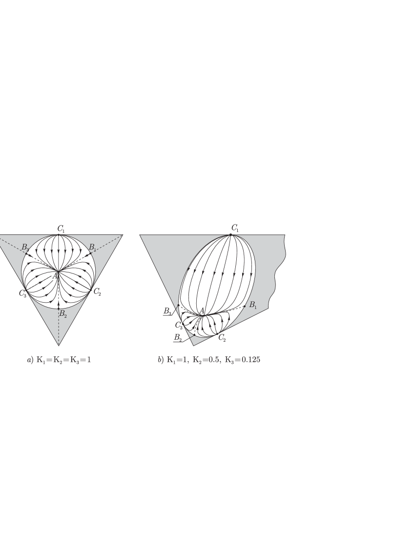
Figure 2: Trajectories of the system (30) on the plane (31) in the case 1^∘.

Let us consider in more detail the structure of the phase portrait in the first case (see figures 2, 3), which, by analogy with vortex dynamics will be referred to as “compact”; clearly, in this case all ratios $M_{i}/M_{j}$ remain bounded for all time. The second (“noncompact”) case can be studied in a similar manner; however, the latter, third case (as well as the case $\sum\mathrm{K}_{i}^{-1}=0$) requires special consideration because, according to (29), an autonomous integral exists in this case.

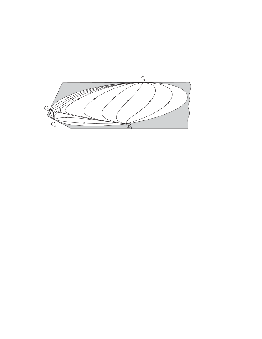
Figure 3: Trajectories of the system (30) on the plane (31) in the case $2^{\circ}$ ($\mathrm{K}_{1}=1$, $\mathrm{K}_{2}=0.5$, $\mathrm{K}_{3}=0.125$).

The structure of the phase flow of the system on the plane (31) is completely determined by its singularities, fixed points, and separatrices connecting fixed points. Statement 1 makes it possible to show that the system on the plane considered here has either four fixed points, which we denote $A$, $B_{1}$, $B_{2}$, and $B_{3}$ (figure 2), or two fixed points — $A$ and $B_{1}$ (figure 3). Point $A$ corresponds to an equilateral homothetic configuration and lies within the domain (ellipse); points $B_{1}$, $B_{2}$, and $B_{3}$ lie on the boundary of the domain and determine collinear homothetic configurations (since it is clear that for these points, $\Delta=0$). Additionally, the system (30) has (in the domain considered) three singularities $C_{1}$, $C_{2}$, and $C_{3}$, which lie on the boundary (32) in the tangent points of planes $x_{i}=0$; they correspond to the situation when the pair of sources merges.

As in the vortex dynamics, in the compact case, we distinguish two cases, in which the portraits qualitatively differ:

1. all intensities have the same sign;

2. two intensities are positive (negative), while the third intensity is negative (positive), and $\mathrm{K}_{1}+\mathrm{K}_{2}+\mathrm{K}_{3}<0(>0)$.

In the case of $1^{\circ}$, as can be seen from figure 2, collinear configurations are saddle points, and the equilateral configuration is a node point (at $\mathrm{K}_{i}<0$, it is a sink, while at $\mathrm{K}_{i}>0$, it is a source), such that all the three separatrices of collinear points enter into it. All the trajectories start (at $\mathrm{K}_{i}<0$) from singularities $C_{1}$, $C_{2}$, and $C_{3}$, do not go beyond the domain limited by the separatrices of collinear points $B_{1}$, $B_{2}$, $B_{3}$, and merge in the fixed point $A$. (At $\mathrm{K}_{i}>0$, the direction of motion along these trajectories should be reversed.)

In the case $2^{\circ}$, the only fixed point $B_{1}$ (corresponding to the collinear configuration) is a source ($\mathrm{K}_{i}<0$); the equilateral configuration now corresponds to a saddle point. Three separatrices of the saddle point end in the singularities $C_{1}$ $C_{2}$, $C_{3}$, respectively, and the fourth separatrix, ends in the fixed point $B_{1}$. A general phase portrait is given in figure 3.

5 Homothetic configurations for $n$ sources

Of great importance in the dynamics of $n$ point vortices are the simplest periodic solutions, i. e., stationary configurations such that vortices rotate around a common center of vorticity without changing their mutual arrangement. Analogous solutions were found in the dynamics of $n$ point sources, with the only difference that the points move along fixed straight lines passing through the center of divergence of the sources so that their configuration remains self-similar at any time. Such configurations will be referred to as homothetic.

Let us show that the following statement is true

Proposition 5 There exists a one-to-one map between the stationary configurations of the dynamics and the homothetic configurations of the dynamics of $n$ point sources.

PROOF

Indeed, for any stationary configuration in a coordinate system with the origin at the vorticity center, the coordinates of vortices are as follows

$$z_{k}(t)=\zeta_{k}e^{i\Omega t},\quad k=1,\ldots,n,$$

where $\Omega$ is the constant angular velocity of rotation of the configuration, and the constant complex numbers $\zeta_{k}$ satisfy the system of algebraic equations:

$$-2\pi\Omega\bar{\zeta_{k}}=\sum_{l\neq k}^{n}\frac{\Gamma_{l}}{\zeta_{k}-\zeta_{l}},\quad k=1\ldots n,$$ (33)

where $\Gamma_{l}$ are the intensities of vortices $\left(\mathrm{A}_{l}=\frac{i\Gamma_{l}}{2\pi}\right)$.

In the case of sources $(\mathrm{A}_{l}=\frac{\mathrm{K}_{l}}{2\pi})$, we similarly find the particular solutions which specify the homothetic configurations in the form

$$z_{k}=\sqrt{c-2\Omega t}\,\zeta_{k},\quad k=1\ldots n,$$

where $\zeta_{k}$ are complex numbers satisfying the system of equations (33), in which the change of variables $\Gamma_{l}\to\mathrm{K}_{l}$ must be made. $\blacksquare$

Note that the solution of the system of algebraic equations (33) is not known, and the problem of finding the homothetic configurations of sources also cannot be solved completely. A some of particular results for stationary configurations in vortex dynamics are summarized in [9].

Remark 6 In celestial mechanics, the homothetic configurations form a particular case of a wider class of homographic configurations, when all points at all times form such configurations, which rotate around a common center of masses. There seems to be no such configurations, other than homothetic, in the source dynamics. As far as we know, the question of existence of such configurations in the case of vortex sources has not been considered.

6 Vortex sources on the sphere

Let us consider a possible generalization of the motion equations of vortex sources (and other singularities in a fluid flow) for the case of a sphere. To do this, we make a stereographic projection of the plane onto the sphere and write the equations of vortex motion on the sphere [1] in complex form.

In the case of the stereographic projection from the southern pole onto the plane passing through the northern pole (see figure 4), the rectangular coordinates of a point on the sphere can be written as

$$\begin{gathered}x=\frac{\xi}{1+\lambda(\xi^{2}+\eta^{2})},\quad y=\frac{\eta}{1+\lambda(\xi^{2}+\eta^{2})},\quad z=R\frac{1-\lambda(\xi^{2}+\eta^{2})}{1+\lambda(\xi^{2}+\eta^{2})},\end{gathered}$$ (34)

where $\lambda={(2R)}^{-2}$ is the curvature.

Using the complex coordinates of vortices $\zeta_{k}=\xi_{k}+i\eta_{k}$, $k=1\ldots n$ on the plane considered, the motion equations of the vortices can be represented in the form

$$\dot{\bar{\zeta}}_{k}=\frac{\left(1+\lambda{|\zeta_{k}|}^{2}\right)^{2}}{2\pi}\left(\sum_{l\neq k}^{n}\frac{i\Gamma_{l}}{\zeta_{k}-\zeta_{l}}-\left(\sum_{l\neq k}^{n}i\Gamma_{l}\right)\frac{\lambda\bar{\zeta_{k}}}{\left(1+\lambda{|\zeta_{k}|}^{2}\right)}\right)\!.$$ (35)

Remark 7 The factor before the second summand in (35) in the book [1] appears to be erroneous.

The velocity of the fluid determined by the vortices in any point of the sphere is expressed analogous to (35):

$$\dot{\bar{\zeta}}=\frac{\left(1+\lambda{|\zeta_{k}|}^{2}\right)^{2}}{2\pi}\left(\sum_{k=1}^{n}\frac{i\Gamma_{l}}{\zeta-\zeta_{l}}-\left(\sum_{l=1}^{n}i\Gamma_{l}\right)\frac{\lambda\bar{\zeta}}{\left(1+\lambda{|\zeta_{k}|}^{2}\right)}\right)\!.$$ (36)

It can be easily shown that the divergence of this velocity field is zero and its vorticity is constant at any point of the sphere $\zeta\neq\zeta_{k}$ and equals

$$\omega=\frac{1}{4\pi R^{2}}\sum_{k=1}^{n}\Gamma_{k}.$$ (37)

By analogy with the planar case, let us replace the intensities $i\Gamma_{k}$ by complex numbers $\mathrm{A}_{k}=\mathrm{K}_{k}+i\Gamma_{k}$; we obtain the equations describing the motion of singularities. These singularities can be interpreted as vortex sources on the sphere.

$$\dot{\bar{\zeta}}_{k}=\frac{\left(1+\lambda{|\zeta_{k}|}^{2}\right)^{2}}{2\pi}\left(\sum_{k=1}^{n}\frac{\mathrm{A}_{k}}{\zeta_{k}-\zeta_{l}}-\left(\sum_{l\neq k}\mathrm{A}_{l}\right)\frac{\lambda\bar{\zeta_{k}}}{\left(1+\lambda{|\zeta_{k}|}^{2}\right)}\right)\!.$$ (38)

Unlike the planar case, the velocity field determined by the singularities (38) (this field can be calculated by formula (36) with replacement $i\Gamma_{l}\to\mathrm{A}_{l}$), in addition to the vortex sources in points $\zeta_{k}$, has a non-zero vorticity (37) and a divergence equal to

$$\kappa=-\frac{1}{4\pi R^{2}}\sum_{l=1}^{n}\mathrm{K}_{l}.$$ (39)

at any point of the sphere $\zeta\neq\zeta_{k}$.

Clearly, such corrections in the motion equations of a fluid on a sphere stem from the compactness of the sphere, and if a point source or a vortex appears in some point, at the same time, a point sink or sinks uniformly distributed over the surface of the sphere must appear somewhere. Equations (38) have not been studied yet. It is still unclear whether they have at least one first integral and whether they are Hamiltonian.

Acknowledgement. We are grateful to M. A. Sokolovskiy for the reference to the work [3] and fruitful discussions. This work was supported in part by CRDF (RU-M1-2583-MO-04), INTAS (04-80-7297), RFBR (04-205-264367) and NSh (136.2003.1).

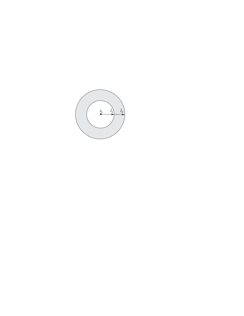
Figure 1:

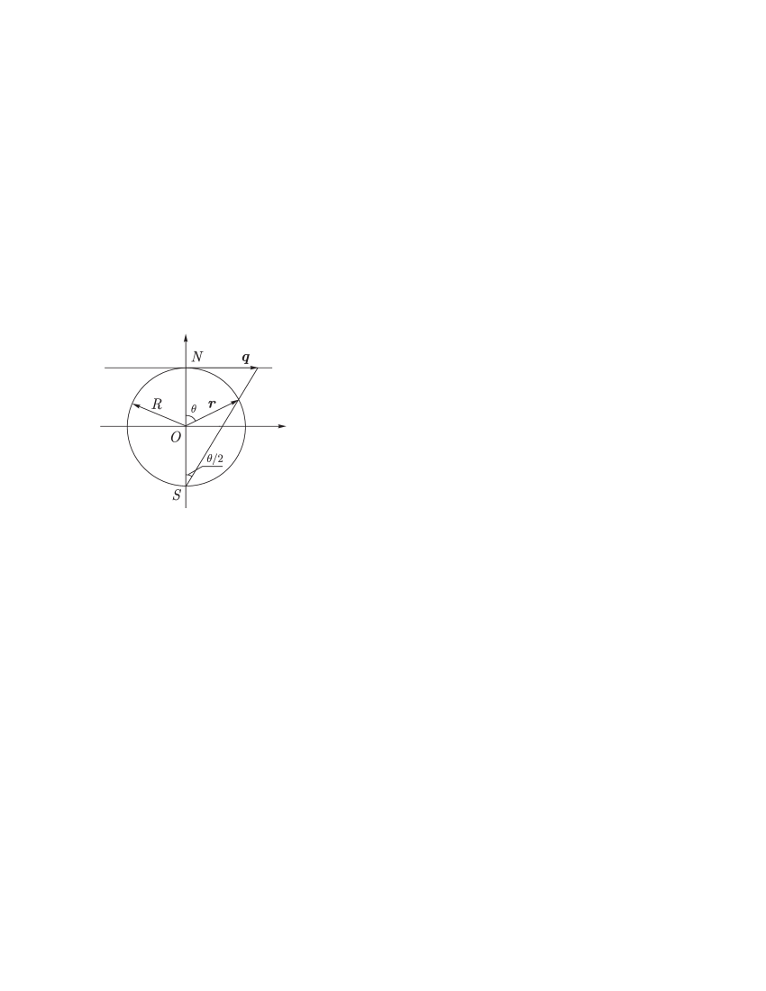
Figure 4:

Figure 1.

Figure 2. Trajectories of the system (30) on the plane (31) in the case 1^∘.

Figure 3. Trajectories of the system (30) on the plane (31) in the case $2^{\circ}$ ($\mathrm{K}_{1}=1$, $\mathrm{K}_{2}=0.5$, $\mathrm{K}_{3}=0.125$).

Figure 4.

References

- [1] Newton P. K. The -Vortex problem: Analytical Techniques, Springer, 2001.
- [2] Fridman A. A., Polubarinova P. Ya. On moving singularities of a flat motion of an incompressible fluid. Geofizicheskii sbornik, 1928, p. 9–23.
- [3] Bogomolov V. A. Motion of an ideal constant-density fluid in the presence of sinks. Izv. Akad. Nauk SSSR. Mekhanika zhidkosti i gaza. 1976, No. 4, p. 21–27.
- [4] Jones S. W., Aref H. Chaotic advection in pulsed source-sink systems. Phys. Fluids, 1988, v. 31(3), p. 469–485.
- [5] Stremler M., Haselton F. R., Aref H. Designing for chaos: applications of chaotic advection at the microscale. Phil. Trans. R. Soc. Lond. A. 2004, v. 362, p. 1019–1036.
- [6] Kirchhoff G. Mechanics. Lectures on mathematical physics. Moscow: Akad. Nauk SSSR, 1962. Transl. from German. Kirchhoff G. Vorlesungen über mathematische Physik. Mechanik, Leipzig, 1874.
- [7] Helmholtz H. Über Integrale hydrodinamischen Gleichungen weiche den Wirbelbewegungen entsprechen. J. Rein. Angew. Math., 1858, v. 55, s. 25–55., see also Russian translation with Chaplygin’s comments in the book Helmholtz G. Fundamentals of vortex theory. – Moscow-Izhevsk: IKI, 2002.
- [8] Borisov A. V., Mamaev I. S. Poisson structures and Lie algebras in the Hamiltonian mechanics. Moscow–Izhevsk: NITs RKhD, 1999.
- [9] Borisov A. V., Mamaev I. S. Mathematical methods of vortex structure dynamics. In “Fundamental and applied problems of vortex theory” (A.V. Borisov, I.S. Mamaev, M.A. Sokolovskiy, Eds.) Collection of papers — Moscow-Izhevsk: IKI, 2003, p. 17-178.