The restricted two-body problem in constant curvature spaces.

Abstract

We perform the bifurcation analysis of the Kepler problem on $S^{3}$ and $L^{3}$. An analogue of the Delaunay variables is introduced. We investigate the motion of a point mass in the field of the Newtonian center moving along a geodesic on $S^{2}$ and $L^{2}$ (the restricted two-body problem). When the curvature is small, the pericenter shift is computed using the perturbation theory. We also present the results of the numerical analysis based on the analogy with the motion of rigid body.

Keywords and phrases: Kepler problem, bifurcation analysis, perihelion shift, Delaunay variables, restricted problem.

1 Problem statement

We start with the equations of motion for a particle of unit mass on a three-dimensional sphere $S^{3}$ or in a Lobachevsky space $L^{3}$ (pseudosphere).

The sphere $S^{3}$ (pseudosphere $L^{3}$) can be parameterized using the Cartesian (redundant) coordinates of the four-dimensional Euclidean space $\mathbb{R}^{4}$ (the Minkovsky space $\mathbb{M}^{4}$) with the constraint

$$\Phi(q)=\frac{1}{2}(g_{\mu\nu}q^{\mu}q^{\nu}\pm R^{2})=\frac{1}{2}(\langle q,q\rangle\pm R^{2})=0$$ (1)

where $g=\text{diag}(1,1,1,1)$ ($g=\text{diag}(-1,1,1,1)$) is the corresponding metrics. Hereinafter, an upper sign in ”$\pm$” is used for the sphere and a lower sign is used for the pseudosphere. The metrics in $\mathbb{R}^{4}$ ($\mathbb{M}^{4}$) generates a metrics in the sphere $S^{3}$ (the Lobachevsky metrics in the pseudosphere $L^{3}$).

In terms of the Cartesian coordinates, the Lagrangian for the particle’s motion in the field of the potential $U(q)$ is

$$\mathcal{L}=\frac{1}{2}g_{\mu\nu}\dot{q}^{\mu}\dot{q}^{\nu}-U(q),$$

with the constraint 1. Using the Hamiltonian formalism for systems with constraints (Arnold et al. 1993), we get

$$\mathcal{H}=\frac{1}{2}\left(\langle p,p\rangle-\frac{\langle p,q\rangle^{2}}{\langle q,q\rangle}\right)+U(q).$$ (2)

Then the canonical equations of motion are $\dot{q}=\displaystyle{\frac{\partial H}{\partial p}}$, $\dot{p}=-\displaystyle{\frac{\partial H}{\partial q}}$.

Two-body problem on $S^{3}$ ($L^{3}$). Consider the two-body problem on the curved spaces $S^{3}$ ($L^{3}$), where bodies are assumed to be point masses. Let these masses move in the field of some potential $U(q_{1},q_{2})$ ($q_{1},q_{2}$ are the coordinates of bodies on $S^{3}$ ($L^{3}$)). In this particular case the potential energy $U$ depends on the distance between two points (this distance is measured along a geodesic). In our case, there is a center of mass frame of reference such that the two-body problem can be reduced to the problem of the particle’s motion in the field of a fixed attracting center (i.e. to the Kepler problem in the case of the Newtonian interaction). The analogue of the Kepler problem is superintegrable on $S^{3}$ ($L^{3}$) (see Kozlov 1994, Borisov et al. 1999 and Killing 1885). The generalization of all the Kepler laws to spaces of constant curvature is given by Kozlov (1994). But in curved spaces the center-of-mass frame of reference does not exist and therefore if the interaction between two bodies is Newtonian-like, the two-body problem is not integrable on $S^{3}$ and $L^{3}$.

In terms of the Cartesian canonical variables $q_{a}$ and $p_{a}$, the Hamiltonian of the two-body system is (the index $a$ denotes the number of the mass $m_{a}$)

$$\mathcal{H}=\frac{1}{2m_{1}}\frac{\langle p_{1},p_{1}\rangle\langle q_{1},q_{1}\rangle-\langle p_{1},q_{1}\rangle^{2}}{\langle q_{1},q_{1}\rangle}+$$

$$\qquad{}+\frac{1}{2m_{2}}\frac{\langle p_{2},p_{2}\rangle\langle q_{2},q_{2}\rangle-\langle p_{2},q_{2}\rangle^{2}}{\langle q_{2},q_{2}\rangle}+U(q_{1},q_{2}).$$ (3)

Invariant manifolds. The three dimensional two-body problem is rather complicated. Therefore by analogy with the planar case, we will examine in detail the motion on the invariant submanifolds of the system . The behavior of the system on invariant submanifolds allows us to make conclusions about some properties of the system (nonintegrability, stochasticity) in the whole phase space. Nevertheless the three-dimensional problem has not been investigated yet.

The invariant manifolds of the n-body problem in $\mathbb{R}^{3}$ are planes and, similarly, if a space is curved, they are spheres $S^{2}$ (pseudospheres $L^{2}$). There is a three-parameter family of such manifolds at any point of $S^{3}$ ($L^{3}$) (see Borisov et al. 1999).

Restricted two-body problem. In the Euclidean space $\mathbb{R}^{3}$ a passage to the limit is possible in the two-body problem as the mass of attracting center goes to infinity while the interaction energy remains finite. There is an inertial frame of reference with origin at the ”heavier” particle, therefore if the potential is Newtonian, the restricted problem is the Kepler problem.

Consider a similar passage to the limit on $S^{3}$ ($L^{3}$). In this case the attracting center moves along a large circle of the sphere (along a geodesic). The second particle (point mass) moves in the field of attracting center and does not affect the motion of the attracting center.

If the origin is at the first particle, the second particle moves in the field of fixed center and gyroscopic forces. The Lagrangian of the system is

$$\mathcal{L}=\frac{1}{2}\dot{q}^{2}+\frac{1}{2}\sum\limits_{\mu,\nu}B_{\mu\nu}\dot{q}_{\mu}{q}_{\nu}+\frac{1}{2}\sum\limits_{\mu,\alpha,\beta}B_{\mu\alpha}{q}_{\alpha}B_{\mu\beta}{q}_{\beta}-V(\mathbf{q}),$$ (4)

where $\mathbf{B}=||B_{\mu\nu}||$ is the angular velocity matrix of the frame of reference. Here, $\mathbf{B}\in so(4)$ (i. e. it is a skew-symmetric matrix) in the case of $S^{3}$ and $\mathbf{B}\in so(3,1)$ in the case of $L^{3}$.

2 Bifurcation analysis of the Kepler problem in curved spaces

Let a particle move in the field of Newtonian-like potential on a sphere $S^{3}$ (pseudosphere $L^{3}$). Using spherical coordinates $q_{0}=R\cos\theta$, $q_{1}=R\sin\theta\cos\varphi$, $q_{2}=R\sin\theta\sin\varphi\cos\psi$ and $q_{2}=R\sin\theta\sin\varphi\sin\psi$, we can write the Hamiltonian as

$$\mathcal{H}=\frac{1}{2mR^{2}}\left(p_{\theta}^{2}+\frac{1}{\sin^{2}\theta}\left(p^{2}_{\varphi}+\frac{p_{\psi}^{2}}{\sin^{2}{\varphi}}\right)\right)-\frac{\gamma}{R}\cot\theta.$$ (5)

Separating variables in (5) gives

$$\alpha_{\psi}=p_{\psi}=\text{const},\quad\alpha_{\varphi}^{2}=p_{\varphi}^{2}+\frac{\alpha_{\psi}^{2}}{\sin^{2}\varphi}=\text{const},$$ (6)

$$E=\frac{1}{2mR^{2}}\left(p_{\theta}+\frac{\alpha_{\psi}^{2}}{\sin^{2}\theta}\right)-\frac{\gamma}{R}\cot\theta,$$ (7)

where $\alpha_{\psi}$ is the projection of the three-dimensional angular momentum vector $\boldsymbol{M}=m\boldsymbol{q}\times\dot{\boldsymbol{q}}$ (here $\boldsymbol{q}=(q_{1},\,q_{2},\,q_{3})$) onto the axis $q_{1}$, $\alpha_{\varphi}^{2}$ is the squared momentum $\boldsymbol{M}^{2}$, $E$ is the energy constant. It is easy to see that the vector $\boldsymbol{M}$ is an integral of motion. (In the case of the Lobachevsky plane, all the trigonometric functions of $\theta$ should be replaced with hyperbolic functions.)

Let us see how the domain of possible motions on $S^{3}$ ($L^{3}$) (hereinafter DPM) depends on the energy constant $E$ and the moment constant $\alpha_{\varphi}$.

We put $r=R\tan\theta$ ($r=R\tan\theta$) in (7). If $E$ and $\alpha_{\varphi}$ are fixed then the DPM are defined as follows

$$\frac{\alpha_{\psi}^{2}}{2m}\left(\frac{1}{r^{2}}\pm\frac{1}{R^{2}}\right)-\frac{\gamma}{r}\leqslant E.$$ (8)

Thus to construct a bifurcation diagram we should consider the quadratic equation

$$\tilde{h}r^{2}+\gamma r-\frac{\alpha_{\varphi}^{2}}{2m}=0,$$ (9)

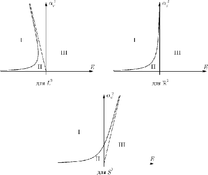
Figure 1: The bifurcation diagrams of the Kepler problem

where $\tilde{h}=E\pm\displaystyle{\frac{\alpha_{\varphi}^{2}}{2mR^{2}}}$. The bifurcation set (i. e. the locus of $(E,\alpha_{\psi})$ at which the domain of possible motion changes topologically) consists of the curves (see Fig. 1)

$$\gamma_{1}:E=\pm\frac{\alpha^{2}_{\varphi}}{2mR^{2}},\quad\gamma_{2}:E=\frac{m\gamma^{2}}{2\alpha^{2}_{\varphi}}\pm\frac{\alpha^{2}_{\varphi}}{2mR^{2}}.$$

If both roots $r_{1}$ and $r_{2}$ of (9) are complex (domain I in Fig. 1) the motion is impossible. If both roots are real and positive (domain II), the possible values of $r$ are given by $r_{1}\leqslant r\leqslant r_{2}$. This implies that a particle moves in the ring $\theta_{1}\leqslant\theta\leqslant\theta_{2}$, with $0<\theta_{1},\,\theta_{2}<\displaystyle{\frac{\pi}{2}}$ for $S^{2}$. If the lower root ($r_{1}$) is negative (domain III), then $r_{2}\leqslant r$ for the real motion on the Lobachevsky plane and $r\leqslant r_{1}$ for the motion on a sphere (since $r$ is negative if $\pi/2\leqslant\theta\leqslant\pi$). It means that on $L^{2}$ a body moves exterior to the circle $\theta\leqslant\theta_{2}$ and if the space is $S^{2}$, a particle moves in the ring $\theta_{1}\leqslant\theta\leqslant\theta_{2}$, where $0<\theta_{1}<\pi/2$, $\pi/2<\theta_{2}<\pi$.

Note that motions on a sphere are bounded because of compactness $S^{3}$. Orbiting time is always finite. Note also that the ”curved” Kepler problems are trajectory isomorphic to their plane analogues, as was shown by Serre (see Appell 1891).

3 Angle-action variables and analogue of Delaunay variables

Define the action variables in terms of spherical variables

$$I_{\psi}=\frac{1}{2\pi}\oint p_{\psi}\,d\psi,\quad I_{\varphi}=\frac{1}{2\pi}\oint p_{\varphi}\,d\varphi,\quad I_{\theta}=\frac{1}{2\pi}\oint p_{\theta}\,d\theta,$$ (10)

where the integral is taken over the whole cycle of the period of motion.

Since $p_{\psi}=\text{const}$ we have from (10) $I_{\psi}=p_{\psi}=\alpha_{\psi}$. The kinetic energy in terms of spherical coordinates on $S^{3}$ is $T=\displaystyle{\frac{1}{2}}(p_{\theta}\dot{\theta}+p_{\varphi}\dot{\varphi}+p_{\psi}\dot{\psi})$, and on the invariant sphere $S^{2}$ where the particle moves, we have $T=\displaystyle{\frac{1}{2}}(p_{\theta}\dot{\theta}+\alpha_{\varphi}\dot{\nu})$; here $\nu$ is a true anomaly (i.e. usual polar angle). Equating these two expressions we get $p_{\varphi}d\varphi=\alpha_{\varphi}d\nu-I_{\psi}d\psi$. The coordinates $\nu$ and $\psi$ change by $2\pi$ per one revolution of the orbit. Therefore, after integrating we have

$$I_{\phi}=\alpha_{\varphi}-I_{\psi}$$ (11)

To compute the third integral of (10), put $r=R\tan\theta$ ($r=R\tan\theta$) and use the equation for the orbit $r(\nu)$ (see Kozlov 1994; Killing 1885).

$$r=\frac{p}{1+e\cos\nu},$$ (12)

where $p=\displaystyle{\frac{\alpha_{\varphi}^{2}}{m\gamma}}$ is a parameter of the orbit, $e=\sqrt{1+\displaystyle{\frac{2\alpha_{\varphi}^{2}}{m\gamma^{2}}\tilde{h}}}$ is the eccentricity. This implies

$$I_{\theta}=\frac{\sqrt{-2m\tilde{h}}}{\pi}\int^{r_{2}}_{r_{1}}\frac{\sqrt{(r-r_{1})(r_{2}-r)}}{r(1\pm r^{2}/R^{2})}\,dr,$$ (13)

where $r_{1}=\displaystyle{\frac{p}{1+e}}$, $r_{2}=\displaystyle{\frac{p}{1-e}}$.

We get after integration

$$I_{\theta}=\sqrt{-2m\tilde{h}}\left(\frac{r_{1}\sqrt{r_{2}^{2}+R^{2}}+r_{2}\sqrt{r_{1}^{2}+R^{2}}}{\sqrt{2\left(\sqrt{(r_{2}^{2}+R^{2})(r_{1}^{2}+R^{2})}+R^{2}+r_{1}r_{2}\right)}}-\sqrt{r_{1}r_{2}}\right)$$

for $S^{3}$, and

$$I_{\theta}=\frac{\sqrt{-2m\tilde{h}}}{2}\left(\sqrt{(R+r_{1})(R+r_{2})}-\sqrt{(R-r_{1})(R-r_{2})}-2\sqrt{r_{1}r_{2}}\right)$$

for $L^{3}$.

Since $r_{1}+r_{2}=-\displaystyle{\frac{\gamma}{\tilde{h}}}$, $r_{1}r_{2}=-\displaystyle{\frac{\alpha_{\varphi}^{2}}{2m\tilde{h}}}$, we get with (11) the explicit expression of the Hamiltonian

$$\mathcal{H}=-\frac{m{\gamma}^{2}}{2(I_{\theta}+I_{\varphi}+I_{\psi})^{2}}\pm\frac{(I_{\theta}+I_{\varphi}+I_{\psi})^{2}}{2mR^{2}}.$$ (14)

Similar to the Euclidean space $\mathbb{R}^{3}$, the Hamiltonian depends only on the sum $I_{\theta}+I_{\varphi}+I_{\psi}$, i.e. the frequencies $\omega_{i}=\displaystyle{\frac{\partial H}{\partial I_{i}}}$, $i=\theta,\,\varphi,\,\psi$, corresponding to the variables $I_{\theta}$, $I_{\varphi}$, $I_{\psi}$, coincide. This is the case of the complete degeneracy, because all the three-dimensional Liouville –Arnold tori foliate into one-dimensional tori i. e. circles. Note that unlike the Hamiltonian in the space $\mathbb{R}^{3}$ (see Markeev 1990), expression 14 has additional terms, which are proportional to $\displaystyle{\frac{1}{R^{2}}}$.

Define new variables $L$, $G$, $H$, $l$, $g$, $h$ (analogues of the Poincare variables)

$$\begin{gathered}L=I_{\theta}+I_{\varphi}+I_{\psi},\quad G=I_{\varphi}+I_{\psi},\quad H=I_{\psi},\\ l=\omega_{\theta},\quad g=\omega_{\varphi}-\omega_{\theta},\quad h=\omega_{\psi}-\omega_{\varphi}.\end{gathered}$$ (15)

In terms of these variables, the Hamiltonian is

$$\mathcal{H}=-\frac{m\gamma^{2}}{2L^{2}}\pm\frac{L^{2}}{2mR^{2}}.$$ (16)

With 16 and 15, we have

$$L=\sqrt{\frac{m\gamma}{-E/\gamma+\sqrt{E^{2}/\gamma^{2}\pm 1/R^{2}}}},\quad G=\alpha_{\varphi},\quad H=\alpha_{\psi}.$$

Equation 16 implies all the Delaunay variables except $l$ are integrals of motion. The angle $l$ is an analogue of the mean anomaly $\zeta$ and changes uniformly with the time $l=\zeta=\displaystyle{\frac{2\pi}{T}}(t-\tau)$. Here $\tau$ is the time, when the particle passes the pericentre, $T$ is the period of orbit revolution, which depends only on the energy constant $E$ (see Killing 1885; Kozlov 1994):

$$T=\pi\sqrt{\frac{m}{\gamma}}R\sqrt{\frac{\pm E/\gamma\pm\sqrt{E^{2}/\gamma^{2}\pm 1/R^{2}}}{E^{2}/\gamma^{2}\pm 1/R^{2}}}.$$

In terms of the angular length of the orbit’s major axis $a$, the energy constant $E=-\displaystyle{\frac{\gamma}{R\tan a}}$ $\left(E=-\displaystyle{\frac{\gamma}{R\tan a}}\right)$.

The Delaunay variables can be expressed in terms of orbit parameters like in the planar case as it shown by Markeev (1990) and Demin et al. (1999). Choose the angular constants so that if we make gnomonic projection $g$, $h$ are the images of the pericentre parameter and the longitude of the ascending node. Denote them by $\omega$ and $\Omega$. Let $\imath$ be the analogue of orbit inclination. This value is equal to the angle between the axis $q_{1}$ and the vector $M$.

Express the variables $L$, $G$, $H$, $l$, $g$, $h$ in terms of the elements of the orbit $p$, $e$, $\imath$, $\tau$, $\omega$, $\Omega$:

$$L =\sqrt{m\gamma R\tan\left(\frac{a}{2}\right)}, \quad l =\zeta,$$ (17)

$$G =\sqrt{m\gamma p}, \quad g =\omega,$$

$$H =\sqrt{m\gamma p}\cos\imath, \quad h =\Omega.$$

In the case of the Lobachevsky space $L=\sqrt{m\gamma R\tan\left(\displaystyle{\frac{a}{2}}\right)}$.

4 Perihelion shift

The observation of Mercury’s perihelion shift is one of the experiments that proves the general relativity theory (GRT) (see Eddington 1963). This shift arises as a result of curving of a space near a gravitating body. Let us prove that in Newtonian mechanics, a Keplerian orbit also precesses in a curved space. Although the laws of precession in these theories are different. We will take the restricted two-body problem as a model problem. This problem is not integrable but if the velocity of the heavier particle is low we can analyze the problem using the perturbation theory. Here we do not mean to give a new physical justification of the perihelion shift, already given in GRT and accepted as classical. We just point out that some phenomena of the practical Celestial Mechanics admit another interpretations (together with the planet nonsphericity, atmosphere refraction and so on). The addition of curvature to the classical Newtonian mechanics is an example of such interpretations.

Consider the restricted two-body problem on $S^{2}$ $(L^{2})$. As usual, the sphere (pseudosphere) is assumed to be embedded in $\mathbb{R}^{3}$ $(\mathbb{M}^{3})$: $\{\boldsymbol{q}=(x,\,y,\,z)|\langle\boldsymbol{q},\,\boldsymbol{q}\rangle=x^{2}+y^{2}\pm z^{2}=\pm R^{2}\}$. Let an attracting center move along the geodesic on $xz$ plane, and we choose the (moving) frame of reference that the attracting center is at the north pole of the sphere (pseudosphere) $\boldsymbol{e}_{3}=(0,\,0,\,1)$. The Lagrangian of point mass (particle of unit mass) is

$$\mathcal{L}=\frac{1}{2}\langle\boldsymbol{\dot{q}},\,\boldsymbol{\dot{q}}\rangle+\gamma\frac{\langle\boldsymbol{e_{3}},\,\boldsymbol{q}\rangle}{\sqrt{R^{2}\mp\langle\boldsymbol{e}_{3},\,\boldsymbol{q}\rangle^{2}}}+\langle\boldsymbol{\dot{q}},\,{\bf B}\boldsymbol{q}\rangle+\frac{1}{2}\langle{\bf B}\boldsymbol{q},\,{\bf B}\boldsymbol{q}\rangle,$$ (18)

here $\bf B$ is the angular velocity matrix of the frame of reference,

$${\bf B}=\left(\begin{matrix}0&0&w\\ 0&0&0\\ \mp w&0&0\end{matrix}\right).$$

Let us assume that the typical size of the domain of motion of the point mass is small in comparison with the radius of curvature $R$. Then we can analyze the problem using perturbation theory. Suppose also that the angular velocity of the attracting center’s motion is small in comparison with the rotation frequency of the point mass moving along the corresponding Keplerian orbit. Take the length $r=R\tan\theta$ $(r=R\tan\theta)$ and azimuth angle $\varphi$ as the coordinates on a sphere (pseudosphere) and transform 18 as

$$\mathcal{L}=\frac{1}{2}\Biggl{(}\frac{\dot{r}^{2}}{\Bigl{(}1{\pm}\displaystyle{\frac{r^{2}}{R^{2}}}\Bigr{)}^{2}}+\frac{{r^{2}}{{\dot{\varphi}}^{2}}}{1{\pm}\displaystyle{\frac{r^{2}}{R^{2}}}}\Biggr{)}+\frac{\gamma}{r}+2\frac{w}{R}\frac{r^{2}\dot{r}}{\Bigl{(}1{\pm}\displaystyle{\frac{r^{2}}{R^{2}}}\Bigr{)}^{2}}\cos\varphi{\mp}\frac{w^{2}}{2}\frac{r^{2}}{1{\pm}\displaystyle{\frac{r^{2}}{R^{2}}}}\sin^{2}\!\varphi.$$ (19)

Here $w=\displaystyle{\frac{v}{R}}$, and $v$ is the linear velocity of the motion of the noninertial frame of reference. If $\displaystyle{R\rightarrow\infty}$, the problem is reduced to the planar Kepler problem.

The terms in 19, which are linear with respect to the velocity, have the order $\displaystyle{\frac{1}{R^{2}}}$ and can not be omitted. To study the evolution of the orbit’s shape in the unperturbed Kepler problem we express the equations 19 in terms of $p$, $\omega$, $e$, $\varphi$. Here, $e$ is the eccentricity, $\omega$ is the longitude of the orbit’s pericenter, $\varphi$ is the azimuth angle, $p$ is the orbit’s parameter, associated with the energy $E$ of the unperturbed Kepler problem by following

$$E=-\frac{1-e^{2}}{2p}\pm\frac{p}{2R^{2}}.$$ (20)

The new variables are expressed in terms of coordinates and velocities (hereinafter $\gamma=1$)

$$r=\frac{p}{1+e\cos(\varphi-\omega)},\quad\frac{r^{2}}{1\pm\displaystyle{\frac{r^{2}}{R^{2}}}}\dot{r}=\frac{e\sin(\varphi-\omega)}{\sqrt{p}},\quad\frac{r^{2}\dot{\varphi}}{1\pm\displaystyle{\frac{r^{2}}{R^{2}}}}=\sqrt{p}.$$ (21)

Hereinafter, for the sake of simplicity, we don’t substitute the expression for $r$ in terms of $p$, $e$, $\omega$, $\varphi$. The Poisson brackets for $p$, $e$, $\omega$, $\varphi$ are

$$\{p,\,e\} =-\frac{4w}{R}\frac{pr^{2}}{1\pm\displaystyle{\frac{r^{2}}{R^{2}}}}\sin\varphi\sin(\varphi-\omega);$$ (22)

$$\{p,\,\omega\} =-2\sqrt{p}+\frac{4w}{R}\frac{pr^{2}}{1\pm\displaystyle{\frac{r^{2}}{R^{2}}}}\sin\varphi\cos(\varphi-\omega);$$

$$\{e,\,\omega\} =\frac{1-e^{2}+\displaystyle{\frac{p^{2}}{R^{2}}}}{e\sqrt{p}}+\frac{4w}{R}\frac{pr}{e\left(1\pm\displaystyle{\frac{r^{2}}{R^{2}}}\right)}\sin\varphi;$$

$$\{p,\,\varphi\} =-2\sqrt{p};$$

$$\{e,\,\varphi\} =-\frac{2\cos(\varphi-\omega)+e+e\cos^{2}(\varphi-\omega)}{\sqrt{p}};$$

$$\{\omega,\,\varphi\} =-\frac{\sin(\varphi-\omega)(2+e\cos(\varphi-\omega))}{e\sqrt{p}},$$

and the Hamiltonian is

$$\mathcal{H}=-\frac{1-e^{2}}{2p}\pm\frac{p}{2R^{2}}\pm\frac{w^{2}}{2}\frac{r^{2}\sin^{2}\varphi}{1\pm\displaystyle{\frac{r^{2}}{R^{2}}}}.$$ (23)

Expressions 22 and 23 imply that when $R\rightarrow\infty$, the variables $p$, $e$, $\omega$ are slow, $\varphi$ is fast. To define the secular change of the orbit’s parameters, when $R\gg r$, we neglect the terms with order higher than $\displaystyle{\frac{1}{R^{2}}}$ and average the equations of motion over the period of unperturbed motion. Averaging over the period is equal to averaging over $\varphi$ with a weight function $\displaystyle{\frac{1}{2\pi}}\int_{0}^{2\pi}f(\varphi)\rho(\varphi)d\varphi$. Here the weight function $\rho$ is defined by the derivative $\dot{\varphi}$ from 21 as $\rho=\displaystyle{\frac{1}{\dot{\varphi}}}$.

So, we have the system:

$$\dot{p} =\mp\frac{v}{R^{2}}\frac{2ep^{7/2}}{(1-e^{2})^{5/2}}\left(\cos\omega+\frac{5}{2}v\frac{e\sqrt{p}\sin\omega\cos\omega}{1-e^{2}}\right),$$ (24)

$$\dot{e} =\pm\frac{v}{R^{2}}\frac{p^{5/2}}{(1-e^{2})^{3/2}}\left(\cos\omega+\frac{5}{2}v\frac{e\sqrt{p}\sin\omega\cos\omega}{1-e^{2}}\right),$$

$$\dot{\omega} =\mp\frac{v}{R^{2}}\frac{p^{5/2}}{(1-e^{2})^{5/2}}\left(\frac{1-2e^{2}}{e}\sin\omega+v\sqrt{p}\left(2-\frac{5}{2}\cos^{2}\omega\right)\right).$$

The equations 24 has the integral

$$-\frac{1-e^{2}}{2p}=C,$$ (25)

This integral implies that there is no secular change of the energy of the unperturbed system 20 to this approximation (Laplace’s theorem).

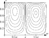
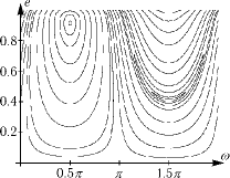
$b=0.1$	$b=1.26$
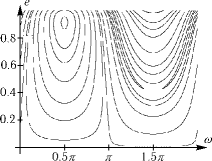
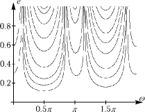
$b=1.27$	$b=25$

Figure 2: Phase portraits of the averaged system

The phase portrait of 24 on the surface of the integral 25 depends on the parameter $b=\displaystyle{\frac{v}{\sqrt{C}}}$. Figure 2 shows the projection of the trajectories onto $(\omega,\,e)$ plane for different values of $b$. The parameter $b$ describes the ratio of the velocity of the attracting center to the characteristic velocity of the particle along the Keplerian orbit. The equation 24 implies that the curvature sign determines the direction of the motion along the trajectory but not the shape of the trajectory. The value of curvature defines the velocity of motion along the trajectory.

It is clear from the figures that the velocity of perihelion shift depends not only on the eccentricity of the orbit but also on the orientation of the orbit with respect to the direction of motion of the attracting center.

If $b$ is small, there exist two stable periodic orbits with the non-zero eccentricity. The main axis of the orbits is perpendicular to the direction of the attracting center’s motion. At pericenter, the direction of the point mass motion along one of the orbit coincides with the direction of the attracting center’s motion $\left(\omega=\displaystyle{\frac{\pi}{2}}\right)$. When the particle moves along another orbit  $\left(\omega=\displaystyle{\frac{3\pi}{2}}\right)$ at the pericenter, its direction is opposite to the direction of the attracting center’s motion. When $b$ increases the orbit with $\omega=\displaystyle{\frac{3\pi}{2}}$ becomes unstable, and if $b$ is sufficiently large, the stable orbit with $\omega=\displaystyle{\frac{\pi}{2}}$ disappears.

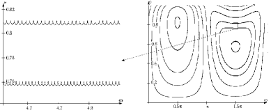
$b=0.5$

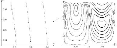
$b=0.9$

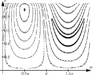
$b=1.2$

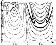
$b=1.5$

Figure 3: Phase portrait of the non-averaged system

The projections of the trajectories of the non-averaged system onto $(\omega,\,e)$ plane are also shown in the figures. Here, we can see small oscillations (for the variables $\omega$, $e$) near the trajectories of the averaged system (see Fig. 3).

Remind that standard explanation of the perihelion shift is based on the Schwarzschield solution (Eddington 1963) and implies that the shift velocity does not depend on the orientation of the orbit $\omega$. This is not the case in our problem statement. There always exist orbits such that only their eccentricities change their values but their pericenters have almost no shift. Moreover, there are fixed points of the system (24), corresponding to the periodic orbits which do not change their form and orientation. Note that the Schwarzschield-like metrics can be constructed if boundary conditions (at infinity) correspond to the space of constant curvature as it shown by Chernikov (1992). And also the restricted two-body problem can be generalized for such metrics. It is clear that the velocity of the perihelion shift depends on both $\omega$ and $e$.

5 Isomorphism with the spherical top dynamics

Consider the restricted two-body problem on the sphere $S^{2}$ in the general case without assumption that the curvature is small. We define the new variables $\boldsymbol{M}$, $\boldsymbol{\gamma}$ using the map ${T^{*}R^{3}\rightarrow e(3)}$, by

$$\boldsymbol{\gamma}=\frac{\boldsymbol{q}}{R},\quad\boldsymbol{M}=\boldsymbol{\gamma}\times\boldsymbol{p}.$$ (26)

Here, the canonical Poisson brackets $\{q_{i},\,p_{j}\}=\delta_{ij}$ are transformed to the Lie –Poisson brackets corresponding to $e(3)$ algebra. The equations of motion are

$$\boldsymbol{\dot{M}}=\boldsymbol{M}\times\frac{\partial\mathcal{H}}{\partial\boldsymbol{M}}+\boldsymbol{\gamma}\times\frac{\partial\mathcal{H}}{\partial\boldsymbol{\gamma}},\quad\dot{\boldsymbol{\gamma}}=\boldsymbol{\gamma}\times\frac{\partial\mathcal{H}}{\partial\boldsymbol{M}},$$ (27)

where the Hamiltonian is

$$\mathcal{H}=\frac{1}{2}\boldsymbol{M}^{2}+(\boldsymbol{M},\,\boldsymbol{w})+U(\boldsymbol{\gamma}),\quad U(\boldsymbol{\gamma})=-\frac{\gamma_{3}}{\sqrt{\gamma^{2}_{1}+\gamma^{2}_{2}}}.$$ (28)

These equations (see Borisov et al. 2001) have two integrals of motion: the area integral $(\boldsymbol{M},\,\boldsymbol{\gamma})=C$ and the geometric integral $(\boldsymbol{\gamma},\,\boldsymbol{\gamma})=1$. In our case $C=0$. Note that this system describes the motion of spherical top in the potential $U(\boldsymbol{\gamma})$ and in the field of gyroscopic forces.

For $\boldsymbol{w}=0$ this system is (super)integrable (the Kepler problem on $S^{2}$), and in this case simple geometric interpretation of the motion exists: the variable $M_{3}=\text{const}$ and the projection of the trajectory onto the plane $(M_{1},\,M_{2})$ is a circle shifted from the origin (incidentally, Hamilton noticed a similar thing, in the two-dimensional Kepler problem). Indeed in the consequence of $(\boldsymbol{M},\vec{\gamma})=0$ we have $\boldsymbol{M}=\dot{\vec{\gamma}}\times\gamma$ and using the equation (12) we obtain

$$\gamma_{1}=\frac{p\cos\nu}{\sqrt{p^{2}+(1+e\cos\nu)^{2}}},\quad\gamma_{2}=\frac{p\sin\nu}{\sqrt{p^{2}+(1+e\cos\nu)^{2}}},$$

$$\gamma_{3}=\frac{1+e\cos\nu}{\sqrt{p^{2}+(1+e\cos\nu)^{2}}},\quad\frac{p^{2}e\dot{\nu}\sin\nu}{(p^{2}+(1+e\cos\nu)^{2})^{3/2}}=M_{3}=const$$

where $\nu$ is a longitude on the sphere $\vec{\gamma}^{2}=1$. Eliminating $\dot{\nu}$ from the last equation we can get

$$M_{1}=-p^{-1}M_{3}(e+\cos\nu),\quad M_{2}=-p^{-1}M_{3}\sin\nu$$

For $\boldsymbol{w}\neq 0$, according to the Liouville–Arnold theorem, an additional integral must exist the system to be completely integrable. We will show soon that in the general case, the additional integral does not exist (see also Borisov et al. 1999, Chernoïvan et al. 1999).

We construct the Poincare map to study the problem numerically. To construct it we use the analogy with the motion of rigid body and choose the Andoyer canonical variables $(L,\,G,\,l,\,g)$ according to Borisov et al. (2001) as

$$\begin{gathered}L=M_{3},\quad l=\arctan\Bigl{(}\frac{M_{2}}{M_{1}}\Bigr{)},\\[-2.84526pt] G=(\boldsymbol{M},\boldsymbol{M}),\quad g=\arccos\left(\frac{-\gamma_{3}}{\sqrt{1-M^{2}_{3}/(\boldsymbol{M},\boldsymbol{M})}}\right).\end{gathered}$$

Then the Hamiltonian as a function of these coordinates is

$$\mathcal{H}=\frac{1}{2}G^{2}+w\sqrt{G^{2}-L^{2}}\cos l+\frac{\sqrt{G^{2}-L^{2}}\cos g}{\sqrt{G^{2}\sin^{2}g+L^{2}\cos^{2}g}}.$$

The equations of motion are canonical:

$$\dot{l}=\frac{\partial\mathcal{H}}{\partial L},\quad\dot{L}=-\frac{\partial\mathcal{H}}{\partial l},\quad\dot{g}=\frac{\partial\mathcal{H}}{\partial G},\quad\dot{G}=-\frac{\partial\mathcal{H}}{\partial g}.$$ (29)

Let us fix the energy level $\mathcal{H}=E$ and define the Poincare section by the relation $g=\displaystyle{\frac{\pi}{2}}$. On this two-dimensional surface we choose the variables $\displaystyle{\frac{L}{G}}$ and $l$ as the coordinates of the Poincare map (similarly to Borisov et al. 2001). The domain of definition of the variables is compact: $l\bmod 2\pi$, $\displaystyle{\left|\frac{L}{G}\right|\leqslant 1}$ and the flow (29) defines corresponding Poincare map.

By direct substitution into 29, it is easily proved that

$$\dot{L}(-L,\,-l,\,G,\,g) =-\dot{L}(L,\,l,\,G,\,g), \quad\dot{l}(-L,\,-l,\,G,\,g) =-\dot{l}(L,\,l,\,G,\,g),$$

$$\dot{G}(-L,\,-l,\,G,\,g) =\dot{G}(L,\,l,\,G,\,g), \quad\dot{g}(-L,\,-l,\,G,\,g) =\dot{g}(L,\,l,\,G,\,g).$$

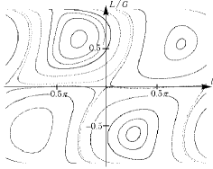
$E=1$, $w=0.1$

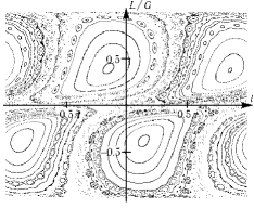
$E=3$, $w=0.1$

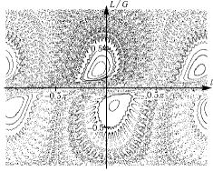
$E=10$, $w=0.1$

Figure 4: The Poincare map for the various energy values and for $w\neq 0$

So, each trajectory $C_{1}$ with the initial conditions $(L_{0},l_{0},$ $G_{0},g_{0})$ corresponds to a similar trajectory $C_{2}$ with initial conditions $(-L_{0},\,-l_{0},\,G_{0},\,g_{0})$, and each point $(L,\,l,\,G,\,g)$ of $C_{1}$ corresponds to a point $(-L,\,-l,\,G,\,g)$ of $C_{2}$. This means the Poincare map (for the chosen section $g=\displaystyle{\frac{\pi}{2}}$ is central symmetric. The phase portraits for the different values of the energy $E$ and parameter $w$ are shown in Fig. 4.

It is easy to see in the figures that the stochastic layer increases as the energy $E$. This proves that the two-body problem in general case is not integrable. The fixed points in Fig. 4 correspond to periodic trajectories of the particle, which play an impotent role in the qualitative analysis of the system.

After the publication of the book by Borisov et al. (1999) and paper by Chernoïvan et al. (1999), at our suggestion, S. L. Ziglin could prove that the additional meromorphic integral does not exist for the potentials that are the analogous to the Newtonian and Hooke interaction for any value of the parameters (see Ziglin 2001 and Ziglin 2003).

6 Hill domains and relative equilibrium

With the equation of motion 27, the integral of energy of the restricted problem 28 can be written as

$$\begin{gathered}\frac{1}{2R^{2}}\boldsymbol{\dot{q}}^{2}+U_{*}(\theta,\varphi)=\mathcal{E}=\text{const},\\ U_{*}=\frac{1}{2}\sin^{2}\theta\sin^{2}\varphi-\mu\cot\theta,\quad\mu=\frac{\gamma}{w^{2}}>0,\quad\mathcal{E}=\frac{E}{w^{2}}+\frac{1}{2},\end{gathered}$$

where $\theta$, $\varphi$ are the spherical coordinates on $S^{2}$ (it means that $\theta$ is a latitude and $\varphi$ is a longitude).

If the energy $E$ is fixed (therefore, $\mathcal{E}$ is also constant) the domain of motion on $S^{2}$ is defined by

$$\mathcal{E}-U_{*}(\theta,\varphi)\geqslant 0.$$ (30)

By analogy with the classical restricted three-body problem (Arnold et al. 1993), we will call this domain the Hill domain of the restricted two-body problem on a sphere.

When the parameters of the system are fixed, the shape of the Hill domains is defined by the singularities and critical points of the effective potential $U_{*}(\theta,\varphi)$. The singularities of $U_{*}$ are at the poles of a sphere. And, since $\mu>0$ and $-\mu\cot\theta\xrightarrow[\theta\to 0]{}\infty$, Hill domain is always not empty, because near $\theta=0$ the inequality (30) holds. Each critical point of the function $U_{*}(\theta,\varphi)$ corresponds to the equilibrium position of the particle (here, the frame of reference rotates with the attracting center). This equilibrium position is usually called a relative equilibrium. Note that (we will prove this below) in the fixed frame of reference the attracting center moves along the large circle and the particle moves along the another circle parallel to the large circle, with it being at the same meridian with the attracting center.

Find the location of critical points by solving the system

$$\frac{\partial U_{*}}{\partial\theta}=\sin\theta\cos\theta\sin^{2}\varphi+\frac{\mu}{\sin^{2}\theta}=0,\quad\frac{\partial U_{*}}{\partial\varphi}=\sin^{2}\theta\sin\varphi\cos\varphi.$$ (31)

We obtain the following results:

1^∘ if $0<\mu<\mu_{*}=\displaystyle{\frac{3\sqrt{3}}{16}}$, there are four critical points on the meridians $\varphi=\displaystyle{\frac{\pi}{2}}$ and $\varphi=\displaystyle{\frac{3}{2}\pi}$ (two points on each meridian). Their latitudes $\displaystyle{\frac{\pi}{2}}<\theta_{1}<\theta_{2}<\pi$ are defined by the equation

$$\frac{1}{2}\sin 2\theta+\frac{\mu}{\sin^{2}\theta}=0;$$

2^∘ if $\mu>\mu_{*}$, the function $U_{*}(\theta,\varphi)$ has no critical points at all.

It is easy to see, that in the case $1^{\circ}$ the critical points $\left(\displaystyle{\frac{\pi}{2},\theta_{2}}\right)$, $\left(\displaystyle{\frac{3\pi}{2},\theta_{2}}\right)$ are the saddle points of the function $U_{*}$, and the points $\left(\displaystyle{\frac{\pi}{2},\theta_{1}}\right)$, $\left(\displaystyle{\frac{3\pi}{2},\theta_{1}}\right)$ are the strict maxima.

Hill domains for both cases (1^∘ and 2^∘) are shown in Fig. 5, 6. It is clear from Fig. 5 that fixed points are in the semisphere opposite to the attracting center. We will use linear approximation to investigate the stability of the obtained fixed points (relative equilibria). Let the point $(\varphi_{i},\theta_{j})$, $i,j=1,2$, be the corresponding fixed point, where $\varphi_{i}\in\{\displaystyle{\frac{\pi}{2},\frac{3}{2}\pi\}}$, $\theta_{j}\in\{\theta_{1},\theta_{2}\}$. According to 31, it is very convenient to parameterize $\mu$ by the latitude of the fixed point:

$$\mu=-\cos\theta_{j}\sin^{3}\theta_{j}.$$ (32)

Since $\mu>0$ for attracting center, $\theta_{j}\in\left[\displaystyle{\frac{\pi}{2}},0\right)$, moreover for $j=1$ $\displaystyle{\frac{\pi}{2}}<\theta_{1}<\theta_{*}$ and these points correspond to the maximum of the effective potential $U_{*}$ and $\theta_{*}<\theta_{2}<\pi$ to the saddle point. Here, $\theta_{*}$ denotes the value of $\theta$, for which $\mu$ 32 reaches the maximum $\mu=\mu_{*}=\displaystyle{\frac{3\sqrt{3}}{16}}$.

Let us introduce canonical impulses $p_{\theta}$, $p_{\varphi}$ corresponding to the spherical angles. In the fixed points their values are $p_{\theta}=0$, $p_{\varphi}=\pm w\cos\theta_{j}\sin\theta_{j}$. Expand the Hamiltonian 28 in the vicinity of the fixed point up to the second power, using the following canonical variables:

$$p_{\theta}=X,\quad p_{\varphi}=\pm w\cos\theta_{j}\sin\theta_{j}+Y,\quad\varphi=\varphi_{i}+y,\quad\theta=\theta_{j}+x.$$

We obtain

$$H=H_{0}+\frac{1}{2}\left(X^{2}+\frac{Y^{2}}{\sin^{2}\theta_{j}}\right)+w\left(yX-\frac{\cos^{2}\theta_{j}}{\sin^{2}\theta_{j}}xY\right)+$$

$$+\frac{1}{2}w^{2}\cos^{2}\theta_{j}\left(\frac{x^{2}}{\sin^{2}\theta_{j}}+y^{2}\right)+\dots,\quad H_{0}=\text{const},\quad j=1,2.$$

The eigenvalues of the corresponding linearized system are

$$\begin{gathered}\lambda_{1,2}=\pm w\sqrt{\frac{1-\cos\theta_{j}-2\cos^{2}\theta_{j}}{1-\cos\theta_{j}}},\quad\lambda_{3,4}=\pm w\sqrt{\frac{1+\cos\theta_{j}-2\cos^{2}\theta_{j}}{1+\cos\theta_{j}}},\\ j=1,\,2.\end{gathered}$$ (33)

The study of the radical expressions in 33 gives us the following results: for $\theta=\theta_{1}$ and $\theta=\theta_{2}$, $\lambda_{3,4}$ are always real and $\lambda_{1,2}$ are real for $\theta=\theta_{1}$ and purely imaginary for $\theta=\theta_{2}$.

This means that

relative equilibria in the restricted two-body problem on a sphere are always unstable.

Note that, according to the theorem of central manifold, the existence of two purely imaginary eigenvalues for the points $\left(\displaystyle{\frac{\pi}{2}},\theta_{2}\right)$ and $\left(\displaystyle{\frac{3}{2}\pi},\theta_{2}\right)$ results in the existence of an unstable (hyperbolic) periodic solution near these points. Fig. 7 shows these solutions for different values of energy.

7 Acknowledgements

This work was supported by RFBR (04-05-64367 and 05-01-01058), CRDF (RU-M1-2583-MO-04), INTAS (04-80-7297) and the program “State Support for Leading Scientific Schools” (136.2003.1).

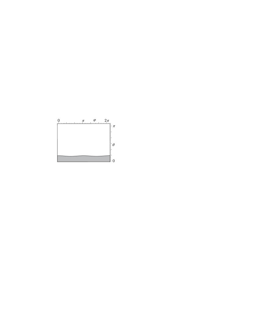
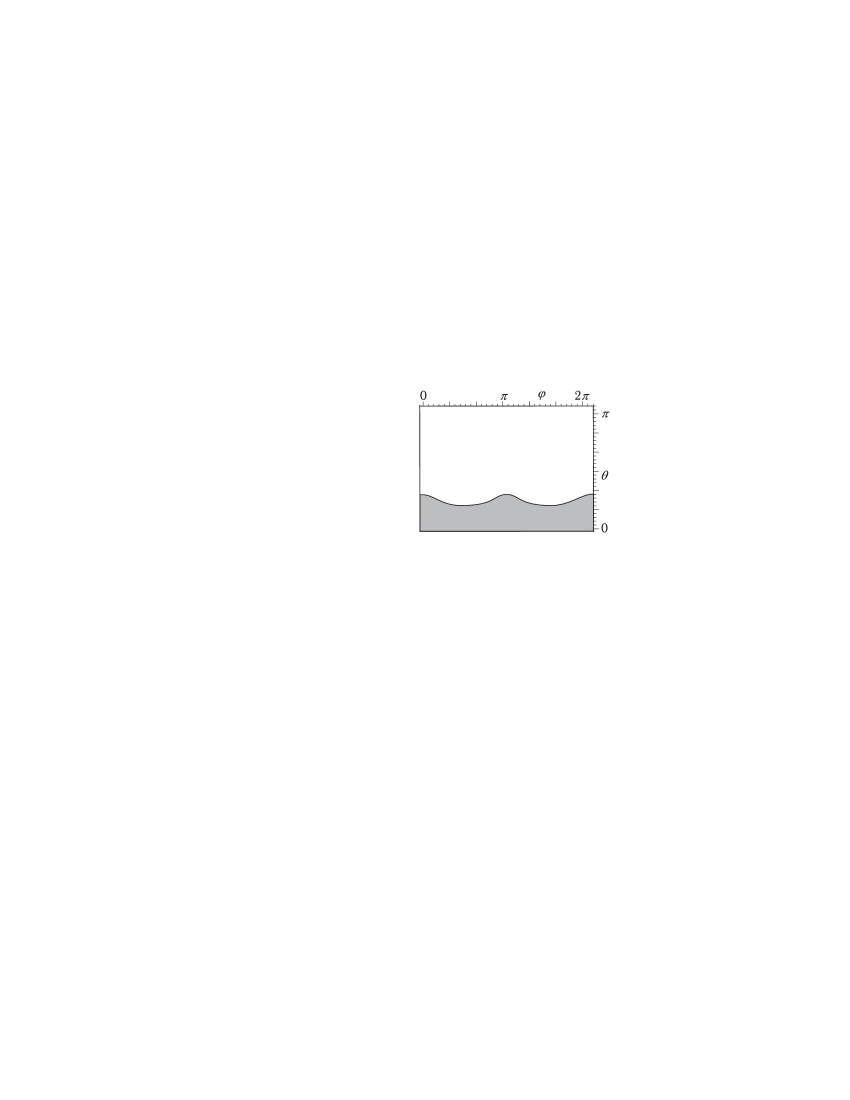
$\mathcal{E}=-0.5$	$\mathcal{E}=-0.2$
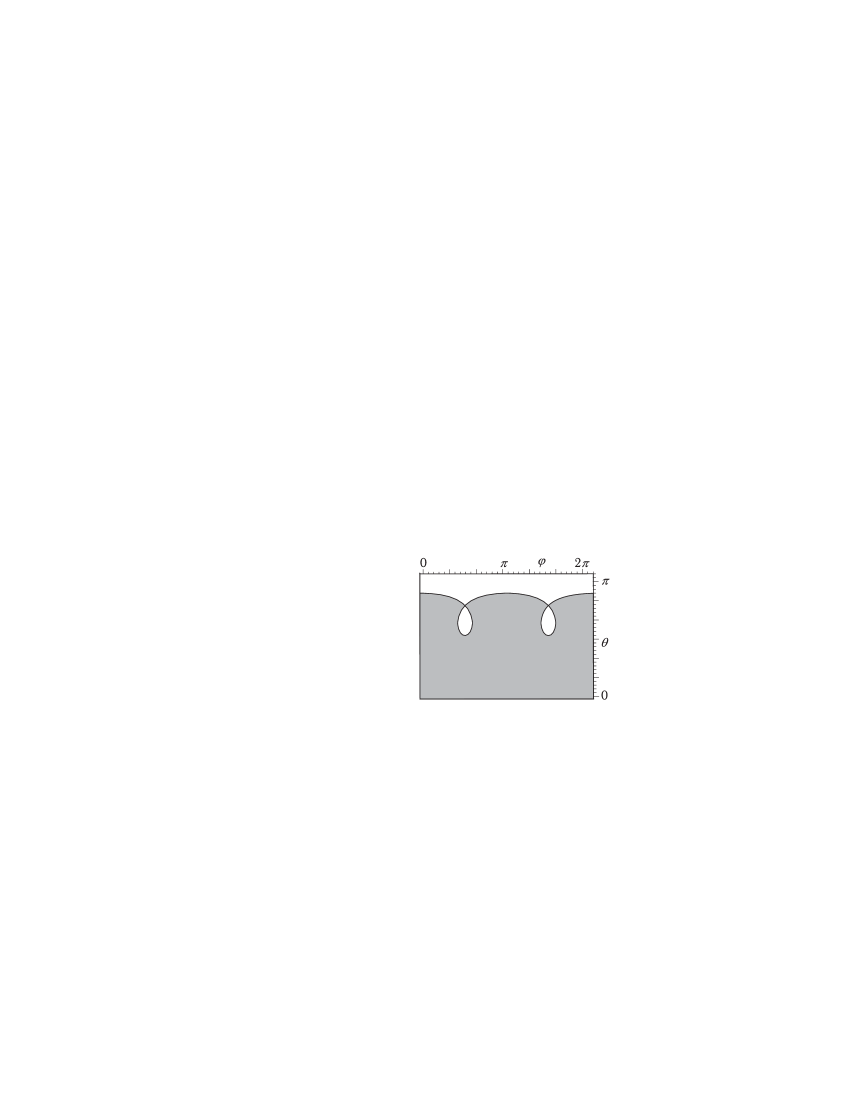
$\mathcal{E}=0$	$\mathcal{E}=0.5$
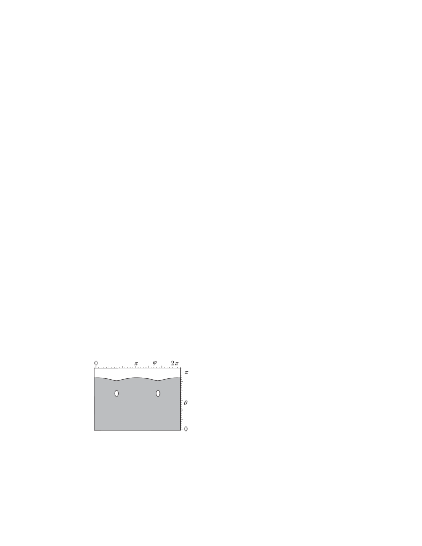
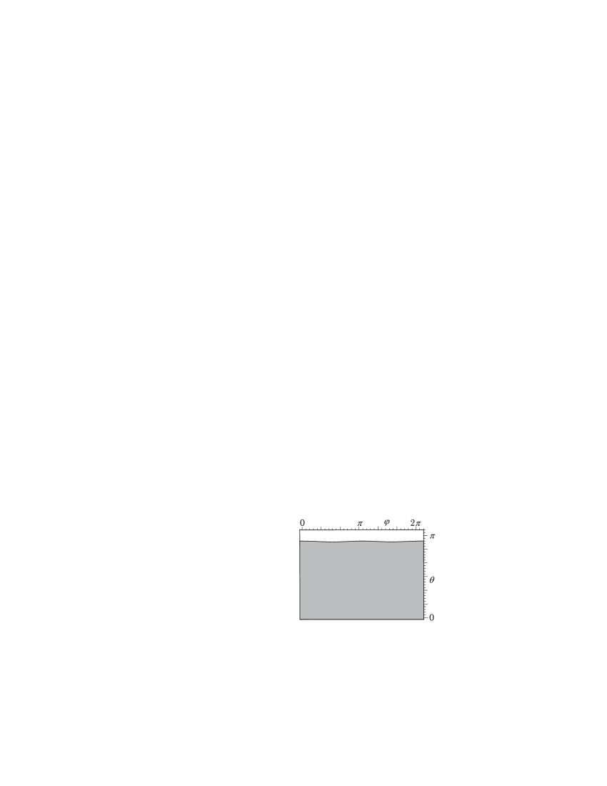
$\mathcal{E}=0.525$	$\mathcal{E}=0.7$

Figure 5: In the case 1^∘ Hill domains (gray shade) for $\mu=0.25<\mu_{*}$ and $w=2.0$

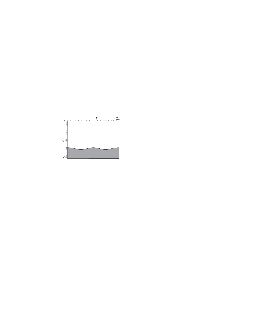
$\mathcal{E}=-0.5$

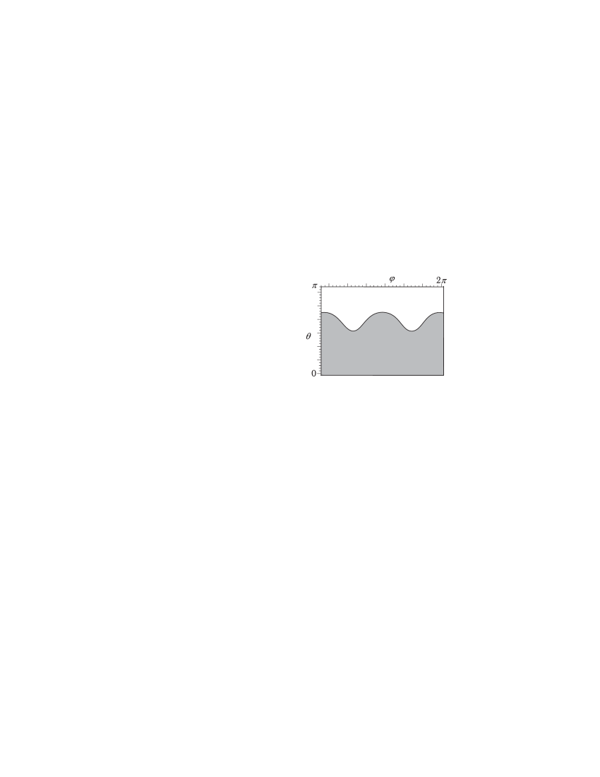
$\mathcal{E}=0.5$

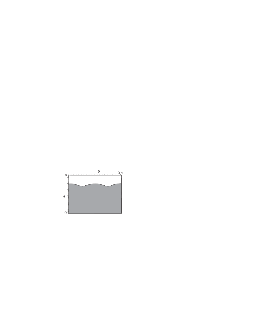
$\mathcal{E}=0.8$

Figure 6: In the case 2^∘ Hill domains (gray shade) for $\mu=0.6>\mu_{*}$ and $w=2.0$

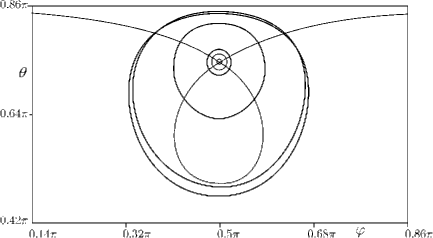
Figure 7: Periodic solutions that appear from the saddle point ($\pi/2$, $\theta_{2}$) (a part of the sphere is shown in the spherical coordinates). The boundary of the Hill domain (see Fig. 5 for $\mathcal{E}=0.5$) is shown for the critical value of the energy $E=0$ when other parameters $w=2$, $\gamma=1$. The values of the energy corresponding to shown orbits are $E$=0.0009, 0.01, 0.027, 0.355, 1.0, 1.024