Chaotic Dynamics of a Free Particle Interacting Linearly with a Harmonic Oscillator

Abstract

We study the closed Hamiltonian dynamics of a free particle moving on a ring, over one section of which it interacts linearly with a single harmonic oscillator. On the basis of numerical and analytical evidence, we conjecture that at small positive energies the phase space of our model is completely chaotic except for a single region of complete integrability with a smooth sharp boundary showing no KAM-type structures of any kind. This results in the cleanest mixed phase space structure possible, in which motions in the integrable region and in the chaotic region are clearly separated and independent of one another. For certain system parameters, this mixed phase space structure can be tuned to make either of the two components disappear, leaving a completely integrable or completely chaotic phase space. For other values of the system parameters, additional structures appear, such as KAM-like elliptic islands, and one parameter families of parabolic periodic orbits embedded in the chaotic sea. The latter are analogous to bouncing ball orbits seen in the stadium billiard. The analytical part of our study proceeds from a geometric description of the dynamics, and shows it to be equivalent to a linked twist map on the union of two intersecting disks.

I Introduction

The one-dimensional free particle and the one-dimensional harmonic oscillator are arguably the two simplest quantum mechanical systems that exist. Nonetheless, and in spite of the intrinsic simplicity of such systems when treated in isolation, the problem of an essentially free particle interacting locally with one or more oscillators is difficult and important to a large class of physical systems. It arises in a variety of contexts, ranging from fundamental studies aimed at understanding the emergence of dissipation in Hamiltonian systems Debievre , to electron-phonon interactions in solids Holstein ; electronphonon , and, more recently, to basic issues associated with the phenomena of quantum decoherence. In the condensed matter literature, in particular, a great deal of theoretical work has focused on the nature of electron-phonon interactions, and the rich variety of behavior that occurs, such as the emergence of “polaronic” quasi-particles. In one version of the well-known Holstein Molecular Crystal Model, a tight-binding electron in a crystal moves between different unit cells, in each of which it interacts with a local oscillator Holstein . Even in the simplest “spin-boson” form of this problem, in which the particle can be conceived as moving between just two sites, and in which it interacts with a single collective oscillator, the problem is not exactly soluble, and has been the subject of intense investigations regarding the appropriateness of various semi-classical approximations SpinBoson .

In this paper we show that the situation can be just as complex in completely classical versions of the problem. We study here the surprisingly rich classical dynamics of what is perhaps the simplest Hamiltonian model that one can think of that incorporates the essential features of this local free particle-oscillator interaction oscillators . Specifically, we consider a single classical particle of mass $m,$ position $x,$ and momentum $p_{0}$ that moves on a ring, the circumference of which is divided into two sections. On one section the particle moves freely, on the other it interacts with a single oscillator of mass $M$ and frequency $\omega$. The associated Hamiltonian we write in the form

$$H=\frac{p_{0}^{2}}{2m}+\frac{P^{2}}{2M}+\frac{1}{2}M\omega^{2}X^{2}-F_{0}X\rho(x),$$ (1)

where $P$ is the oscillator momentum, and $F_{0}$ describes the strength of the interaction, which is linear in the oscillator coordinate $X$, but not in the particle position $x$. In the Hamiltonian (1), $\rho(x)$ is a form factor localized around $x=0$ that describes the range of the interaction. We take $\rho$ to equal unity throughout the interaction region $\left|x\right|\leq\hat{\sigma}$, and to vanish on the section of the ring $\hat{\sigma}+\hat{L}/2>\left|x\right|>\hat{\sigma}$ lying outside this range. With this choice, except at those moments of the evolution when the particle arrives at $x=\pm\hat{\sigma}$, the particle and the oscillator are effectively uncoupled, and evolve independently. At “impacts”, i.e., when the particle arrives at the edges of the interaction region, the particle receives an impulsive kick from the oscillator that conserves the total energy of the system. After each such kick, the particle again moves as a free particle either inside or outside of the interaction region. It is this essentially uncoupled evolution of the two subsystems between impulsive kicks of the particle at $x=\pm\hat{\sigma}$ that makes it possible to numerically and analytically track the dynamics.

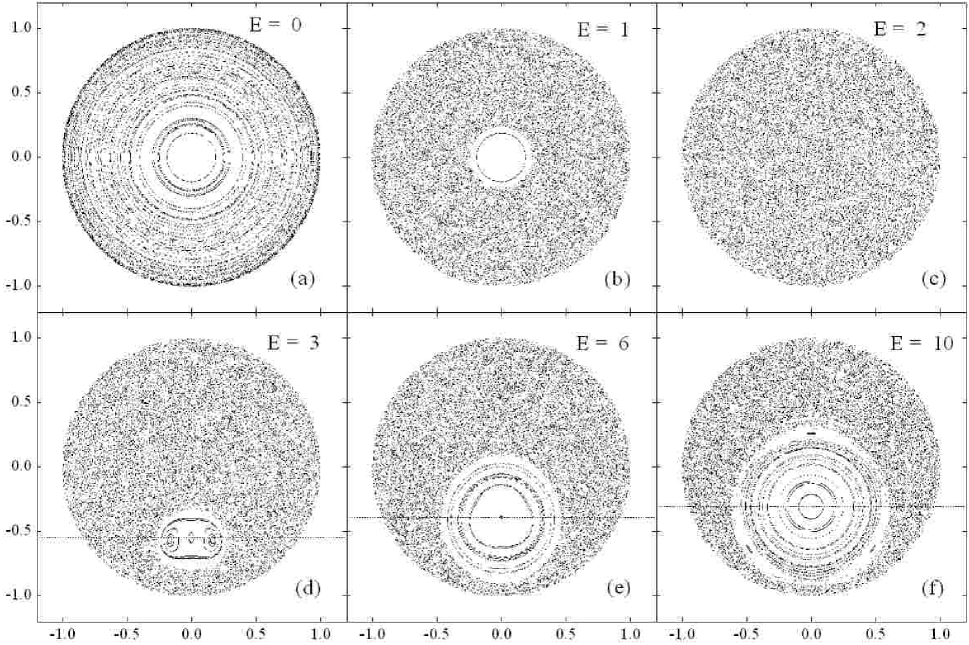
Figure 1: Oscillator phase space diagrams for a system with $\alpha=2$ and $L=4.74$, and varying values of the energy $E=0,1,2,3,6,$ and $10$, as shown (See Sec. II for the definition of the reduced parameters used). The vertical axis in each figure is the scaled oscillator coordinate $\zeta-d$, and the horizontal axis the reduced oscillator momentum $\eta$ defined in Eq. 13.

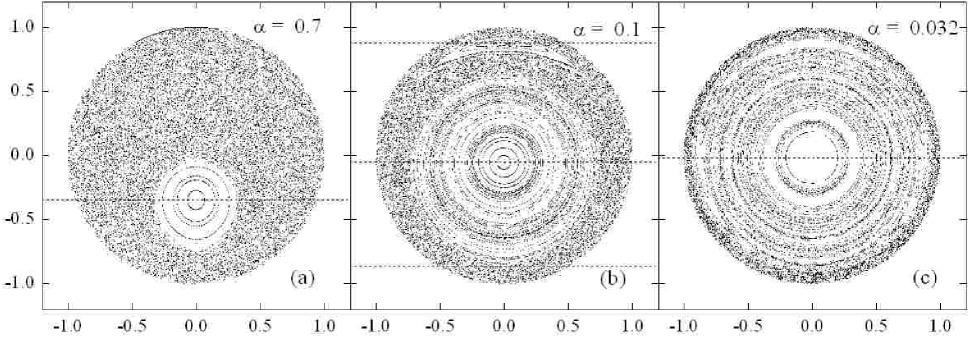
Figure 2: Oscillator phase space diagrams for a system with $E=0.85$ and $L=2$, and values of the coupling strength $\alpha=0.7,0.1$, and $0.032$ (See Sec. II for the definition of the reduced parameters used). The vertical axis in each figure is the scaled oscillator coordinate $\zeta-d$, and the horizontal axis the reduced oscillator momentum $\eta$ defined in Eq. 13. The prominent elliptic island in these figures is what is referred to in the text as Void II. In the last two figures other secondary KAM structures appear at the edges of the Void.

Despite its apparent simplicity, and as can be seen in the numerically determined phase plots appearing in Figs. 1-4, the model has a striking combination of features that are not often seen together in a single closed Hamiltonian system. First, for any given system parameters, the phase space has a very simply described, completely integrable region of controllable size for all energies ranging from that of the ground state, $\hat{E}_{g}=-F_{0}^{2}/2M\omega^{2}$, up to a critical positive energy $\hat{E}_{c}=|\hat{E}_{g}|$ (See Fig. 1 (a) and Fig. 1 (b)). For small positive energies the region of phase space outside of this region, which we refer to as Void I, appears in our numerical calculations to be fully chaotic, with no secondary KAM structures, even very close to the edge of the Void (See, e.g., Fig. 1(b)). This then makes for the simplest possible mixed phase space structure, in which motions in the completely integrable region and in the chaotic region are clearly separated and independent of one another. We are unaware of other Hamiltonian systems which exhibit this clean separation, although it does appear in a piecewise linear symplectic map on the torus that was explicitly constructed to exhibit this property MP .

As a second striking feature of the model, we identify one-parameter families of marginally unstable periodic orbits, that appear as circular arcs in the oscillator phase space (See Fig. 9), and are similar to the so-called bouncing ball orbits that arise in the stadium billiard.

We furthermore show that for fixed, suitably-chosen system parameters, the statistical properties of the dynamics on the different energy surfaces can vary greatly. For some values of the energy, the dynamics is completely integrable, whereas for others it is fully chaotic or displays a mixed, KAM-type behavior. Among the rich variety of structures that arise, we identify and locate the central fixed point of a KAM-type elliptic island that we refer to as Void II. In some cases Void II appears alone, as in Fig. 1(d)-(f) and Fig. 2, while in others Void I and Void II both appear, as in Fig. 4(b) and 4(c). Finally, in the limit of small coupling strengths $F_{0}$, the phase space displays typical KAM structures of the type that generally occur when a completely integrable motion is subject to a small nonlinear perturbation, as in Fig. 2. This, however, by no means exhausts the variety of structures that seem to appear (See Fig. 5).

The presence of chaos in our coupled particle-oscillator model can be understood intuitively as follows. A trajectory of the combined system will tend to be unstable whenever the time the particle takes between two impacts at $x=\pm\hat{\sigma}$ is long compared to the oscillator period. Indeed, when the particle goes slowly, a small change in its velocity at one impact will lead to a large change in the relatively fast moving oscillator coordinate at the next impact. As a result, the height of the potential barrier the particle meets at that moment becomes highly unpredictable, and this is the source of the instability. That this simple picture is in agreement with observed behavior can be seen in Fig. 3, in which it is clear for a given $F_{0}$ and $\hat{L}$ (represented in that figure by the dimensionless parameters $\alpha$ and $L$ introduced in the next section), that the fraction of phase space outside Void I that is chaotic tends to increase as the total energy of the system (and thus the particle speed) decrease. Similarly, increasing $\hat{L}$ tends to increase the chaotic fraction of phase space outside of Void I, since for larger $\hat{L}$ the particle spends more time between succesive visits at $x=\pm\hat{\sigma}$ whenever it is outside the interaction region. A more precise and quantitative analysis of the mechanism leading to chaos in this model will be given in Sec. III, where we will show that the dynamics can be analyzed in terms of a discontinuous linked twist map on the union of two intersecting disks. This is a generalization of the linked twist maps on the torus introduced and studied in TwistMap .

The rest of the paper is laid out as follows. In the next section, we simplify the Hamiltonian (1) by reducing the six system parameters with which it is associated down to two. Following this reduction, we present phase-space plots of the results of a numerical integration of the equations of motion for the system. In Sec. III, we develop a geometric description of the dynamics that makes it relatively straightforward to explain the main features seen in numerical studies, including the emergence of chaos at positive energies (Sec. IV), the existence of islands of regular motion of two different generic types, which we refer to as Void I and Void II (studied in Secs. V and VI, respectively), and the presence of arcs of marginally stable periodic orbits that appear as sets of zero measure in the chaotic portions of our phase space diagrams (Sec. V). In addition, we analytically demonstrate the existence of unstable isolated periodic orbits of arbitrarily large period (Sec. VI). In the last section, we summarize our results, and comment on their ramifications.

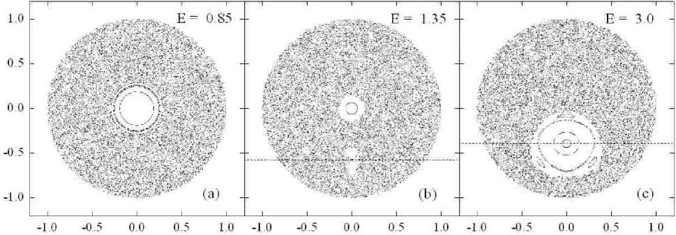
Figure 3: Oscillator phase space diagrams for a system with $\alpha=2$ and $L=2.105$, and energy $E=0.85,1.35$, and $3$. The vertical axis in each figure is the scaled oscillator coordinate $\zeta-d$, and the horizontal axis the reduced oscillator momentum $\eta$ defined in Eq. 13.

II Dimensional Reduction of the Hamiltonian

The system described by the Hamiltonian $H(x,p_{0},X,P)$ as given in (1) depends upon six system parameters: the two masses $m$ and $M,$ the oscillator frequency $\omega,$ and the coupling strength $F_{0},$ as well as the widths $2\hat{\sigma}$ and $\hat{L}$ of the interacting and non-interacting sections of the ring on which the particle moves. To reduce the number of inessential parameters in the system, we now introduce a dimensionless time $\tau=\omega t,$ and dimensionless variables and momenta

$$\tilde{p}=\frac{p_{0}}{\sqrt{m\hbar\omega}}\qquad\tilde{q}=\sqrt{\frac{m\omega}{\hbar}}x,\qquad\tilde{\Phi}=\sqrt{\frac{M\omega}{\hbar}}X,\qquad\tilde{\Pi}=\frac{P}{\sqrt{M\hbar\omega}}$$ (2)

where $\hbar$ is an arbitrary constant having units of action that plays no part in the subsequent dynamics. The new variables obey the equations of motion

$$\frac{d\tilde{q}}{d\tau} =\tilde{p}\qquad\frac{d\tilde{p}}{d\tau}=\tilde{\alpha}\tilde{\Phi}\frac{d\tilde{\chi}}{d\tilde{q}}\left(\tilde{q}\right)$$

$$\frac{d\tilde{\Phi}}{d\tau} =\tilde{\Pi}\qquad\frac{d\tilde{\Pi}}{d\tau}=-\tilde{\Phi}+\tilde{\alpha}\tilde{\chi}(\tilde{q})$$ (3)

which are the canonical equations generated by a transformed Hamiltonian $\tilde{H}_{\tilde{\alpha}}=H/\hbar\omega$, where

$$\tilde{H}_{\tilde{\alpha}}=\frac{1}{2}\left(\tilde{p}^{2}+\tilde{\Pi}^{2}+\tilde{\Phi}^{2}\right)-\tilde{\alpha}\tilde{\Phi}\tilde{\chi}(\tilde{q}),$$ (4)

$\tilde{\alpha}=\sqrt{F_{0}^{2}/M\hbar\omega^{3}},$ and the function $\tilde{\chi}(\tilde{q})=\rho(\tilde{q}\sqrt{\hbar/m\omega})$ vanishes outside the interaction region extending between $\tilde{q}=\pm\sigma\equiv\pm\hat{\sigma}\left(m\omega/\hbar\right)^{1/2}.$ Explicitly, we write

$$\tilde{\chi}\left(\tilde{q}\right)\equiv\chi\left(\tilde{q}/\sigma\right)=\theta\left(\frac{\tilde{q}}{\sigma}+1\right)-\theta\left(\frac{\tilde{q}}{\sigma}-1\right)$$ (5)

where $\theta\left(x\right)$ is the Heaviside step function. This form for the function $\chi$ allows an additional simplification through the scale transformation

$$q=\tilde{q}/\sigma\qquad p=\tilde{p}/\sigma\qquad\Phi=\tilde{\Phi}/\sigma\qquad\Pi=\tilde{\Pi}/\sigma.$$ (6)

With a suitable redefinition of the coupling constant $\tilde{\alpha}=\alpha\sigma$, we obtain the following one parameter family

$$H_{\alpha}=\frac{1}{2}\left(p^{2}+\Pi^{2}+\Phi^{2}\right)-\alpha\Phi\chi(q)$$ (7)

of reduced Hamiltonians $H_{\alpha}=\tilde{H}_{\tilde{\alpha}}\sigma^{-2}$ describing the system, where now the interaction region is associated with the fixed interval $q\in\left[-1,1\right]$. Note that in this form the dimensionless coupling constant

$$\alpha=\sqrt{|\hat{E}_{g}|/\frac{1}{2}{m\hat{\sigma}^{2}\omega^{2}}}$$ (8)

involves the ratio of the (original) ground state energy of the system to the kinetic energy of a particle that crosses the interaction region in one oscillator period.

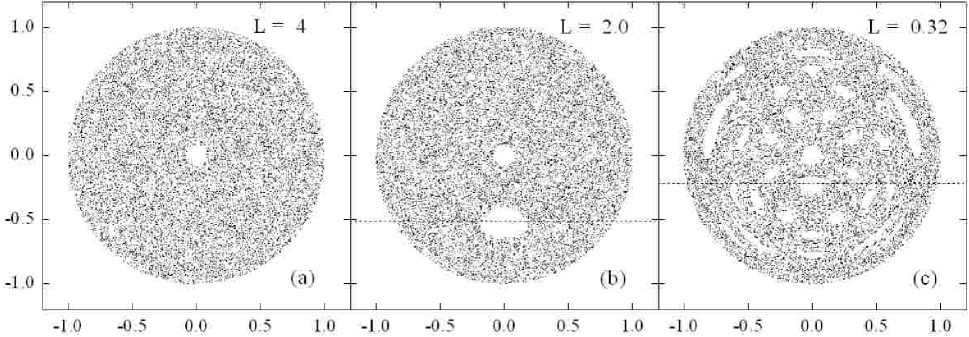
Figure 4: Oscillator phase space diagrams for a system with $E=1.6$ and $\alpha=2$, and values of the length $L=4,2,$ and $0.32$, of the non-interacting region as shown (See Sec. II for the definition of the reduced parameters used). The vertical axis in each figure is the scaled oscillator coordinate $\zeta-d$, and the horizontal axis the reduced oscillator momentum $\eta$ defined in Eq. 13. At the center of each of these figures is a small Void I. As $L$ is decreased, Void II appears and then ascends toward the impenetrable Void I. The collision between these two elliptic islands appears to generate considerable structure.

We have thus reduced the number of system parameters down to the single explicit parameter $\alpha$ describing the coupling strength, and one additional parameter $L=\hat{L}/\hat{\sigma}$ associated with the total range $2+L$ of the particle coordinate $q$. We note in passing that with this choice for the function $\chi\left(q\right),$ the coupling parameter is equal to the equilibrium value $\Phi_{\text{eq}}^{\text{in}}=\alpha$ of the oscillator coordinate when the particle is in the interaction region $q\in\left[-1,1\right],$ and that the ground state, which now has rescaled energy $E_{g}=-\alpha^{2}/2,$ occurs when the particle and the oscillator are both at rest, with the particle in the interaction region.

The equations of motion corresponding to (7)

$$\dot{q} =p\qquad\qquad\dot{p}=\alpha\Phi\left[\delta\left(q+1\right)-\delta\left(q-1\right)\right]$$

$$\dot{\Phi} =\Pi\qquad\qquad\dot{\Pi}=-\Phi+\alpha\chi\left(q\right),$$ (9)

with dots denoting derivatives with respect to $\tau$, show that the particle feels an impulsive force only when it reaches the edges of the interaction region, but otherwise travels as a free particle. The particle’s momentum undergoes discontinuous changes at these moments, but its position remains a continuous function of time. The impulse imparted to the particle at $q=\pm 1$ is readily computed from the oscillator displacement using only conservation of total energy. When the particle enters the interaction region, the oscillator experiences an interaction force of finite magnitude $\alpha$ that suddenly shifts the equilibrium position about which it oscillates from $\Phi_{\text{eq}}^{\text{out}}=0$ to $\Phi_{\text{eq}}^{\text{in}}=\alpha$, but the amplitude and momentum of the oscillator remain continuous functions of time. Thus, when the particle is in the interaction region, the oscillator phase point $\left(\Phi\left(\tau\right),\Pi\left(\tau\right)\right)$ rotates at unit angular speed about the equilibrium state $\left(\Phi,\Pi\right)=\left(\alpha,0\right),$ and when the particle is outside the interaction region, a similar free rotation takes place about the origin of the oscillator phase plane. As mentioned in the introduction, it is this essentially uncoupled evolution of the two subsystems between impulsive kicks of the particle at $q=\pm 1$ that makes it straightforward to numerically and analytically track the resulting dynamics.

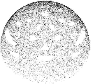
Figure 5: Visualization of the Poincaré section at $x=0$ of the energy surface for a particle-oscillator system with $E=1.6$, $\alpha=2$, and $L=0.32$ (See Sec. II for the definition of the reduced parameters used). We display phase points generated, as described in the text, for 100 initial conditions randomly chosen on the energy surface. The same data appear in Fig. 4(c). This representation of the energy surface is as seen by an observer located outside the energy surface, upside down in the $\Pi$-$p$ plane.

As in any system with two degrees of freedom, the energy surfaces associated with (7) are three dimensional. Their two-dimensional sections at $q=0$ are ellipsoids centered at $\left(\Phi,\Pi,p\right)=\left(\alpha,0,0\right).$ In Fig. 5 we display phase points recorded on the Poincaré section at $q=0$ and $p>0$ arising from the numerically determined evolution of 100 initial conditions randomly chosen on such an energy surface and evolved for a time corresponding to 500 passages through the section. Note that the Hamiltonian (7) is invariant with respect to the parity operation of the particle. Thus, if $\left(\Phi\left(t\right),\Pi\left(t\right),p\left(t\right),q\left(t\right)\right)$ is a solution to the equations of motion, so is $\left(\Phi\left(t\right),\Pi\left(t\right),-p\left(t\right),-q\left(t\right)\right)$, and for symmetrized pairs of randomly chosen initial conditions, the corresponding set of phase points recorded at $-p$ will be the same as at $p,$ i.e., the back half of the ellipsoid, if displayed, would be a mirror image of the front half. This symmetry, together with time reversal invariance explains the additional $\Pi\rightarrow-\Pi$ symmetry that our phase plots exhibit.

As a result it therefore suffices to represent the evolution by simply recording the oscillator phase point $\left(\Phi\left(t\right),\pi\left(t\right)\right)$ each time that $q=0$ and $p$ is positive. Such a representation is obtained by numerically computing the return map for this Poincaré section, and has been used in Figs. 1-4 and 9.

III Geometric Description of the Dynamics

Although the dynamics of the system recorded at $q=0$ shows most clearly the inherent symmetries of the system, to actually explain the features that appear in our phase plots, it is obviously necessary to consider those times at which the particle reaches the edges of the interaction region at $q=\pm 1$. At fixed energy $E$, and with the position $q=\pm 1$ of the particle determined up to a sign, the state of the system at these moments is also conveniently represented as a point in the $\Phi-\Pi$ oscillator phase plane. In general, at a given $E>0$, the available phase space for the oscillator when the particle is in the interaction zone is a disk $D_{-}(E)$ of radius $\sqrt{2E+\alpha^{2}}$ centered at the point $(\alpha,0)$ in the $\left(\Phi,\Pi\right)$ plane, that obviously contains the origin of the phase plane. Similarly, when the particle is outside the interaction zone, the available phase space for the oscillator is a disk $D_{+}(E)$ of radius $\sqrt{2E}$ centered at the origin. Any point $\left(\Phi,\Pi\right)$ in the set $S_{\text{in}}\left(E\right)=D_{-}(E)\setminus D_{+}(E),$ i.e., inside $D_{-}(E)$ but outside $D_{+}(E),$ corresponds to a state with the particle definitely inside the interaction region, and any point in $S_{\text{out}}\left(E\right)=D_{+}\left(E\right)\setminus D_{-}\left(E\right)$ to a state with the particle definitely outside the interaction region. Depending on the energy and the coupling constant, two distinct situations can occur: either the disk $D_{+}\left(E\right)$ does not contain the center of $D_{-}\left(E\right)$, which occurs for $E<\alpha^{2}/2,$ and is depicted in Fig. 6(a), or it does contain the center of $D_{-}\left(E\right)$, which occurs when $E>\alpha^{2}/2$ and is depicted in Fig. 6(b). It should be obvious from the geometry of both figures that the circles which form the edges of the two disks always intersect on the $\Pi$ axis. In the following, given a point $X=(\Phi,\Pi)$, we denote by $A_{\pm}$ its distance from the center of $D_{\pm}(E)$. Physically, $\frac{1}{2}A_{+}^{2}=\frac{1}{2}\left(\Phi^{2}+\Pi^{2}\right)$ is the uncoupled oscillator energy.

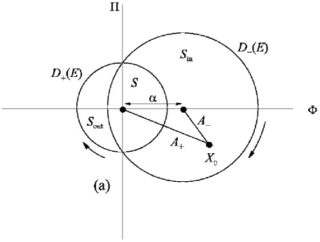
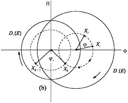
Figure 6: The oscillator phase plane showing the disks $D_{+}(E)$ and $D_{-}(E)$ for (a) $E<\alpha^{2}/2$, and (b) for $E>\alpha^{2}/2$. On these figures the horizontal axis corresponds to the oscillator coordinate $\Phi$ and the vertical axis to the oscillator momentum $\Pi$.

We can now give a simple qualitative description of the motion of the system in geometric terms (see Fig. 6(b)). Suppose that, for fixed $E>0,$ the system is such that at $t=0$ the particle is on the left edge of the interaction zone and moving inward, i.e., $q(0)=-1$ and $\dot{q}(0)>0,$ so that $X_{0}=(\Phi_{0},\Pi_{0})\in D_{-}(E)$. As the particle now crosses the interaction region to $q=1$, the oscillator phase point simply rotates on a circular arc around the point $(\alpha,0)$ through an angle that, in our dimensionless units, can be written

$$\varphi_{-}(A_{-})=\frac{2}{\dot{q}(0)}=\frac{2}{\sqrt{2E+\alpha^{2}-A_{-}^{2}}},$$ (10)

where the second form follows through energy conservation. Note that the rotation angle depends monotonically on the radius of the circle on which the phase point moves, so that two nearby phase points at different radii will rotate through different angles. In this way a shear $T_{-}$ is induced on the disk $D_{-}\left(E\right).$ Since the angle $\varphi_{-}(A_{-})$ diverges as $A_{-}$ approaches the radius of $D_{-}(E)$, the strength of the shear diverges near the edge, and the dynamics becomes increasingly sensitive to small changes in $A_{-}$.

If the new phase point $X_{1}$ so obtained lies in $S_{\text{in}}\left(E\right),$ the particle encounters a potential energy barrier at $q=1$ that is greater than its kinetic energy. Consequently, it reflects from the barrier, reversing its motion to cross the interaction region back to $q=-1,$ during which time the oscillator phase point continues its rotation about the center of $D_{-}(E)$, through the same angle $\varphi_{-}(A_{-})$. The process then repeats itself, generating a sequence of oscillator phase points $X_{1},X_{2,},\ldots$ separated by equal angular displacements $\varphi_{-}(A_{-})$ until, for some $k,$ the phase point $X_{k}$ falls inside $S\left(E\right).$

At such a time, the particle has sufficient kinetic energy to overcome the barrier it encounters, and passes out of the interaction region with a new kinetic energy equal to $E-\frac{1}{2}A_{+}^{2},$ where $A_{+}$ is the distance between the point $X_{k}$ and the origin (the center of the disk $D_{+}\left(E\right)$). The particle then travels through a distance $L$ around the outer section of the ring, and arrives again at $q=\pm 1,$ while the oscillator phase point rotates on the second disk $D_{+}\left(E\right)$ through an angle

$$\varphi_{+}(A_{+})=\frac{L}{\sqrt{2E-A_{+}^{2}}}$$ (11)

about the origin of the phase plane. Thus, a different shear $T_{+}$ is induced on the disk $D_{+}\left(E\right)$. The new phase point $X_{k+1}$ so obtained is depicted in Fig. 6(b). Obviously this way of depicting the evolution can be repeated indefinitely, and provides an efficient way to analyze and explain various features of the dynamics.

IV The Emergence of Chaos

For example, the description given in the last section makes it clear that the mechanism underlying the appearance of chaos in this system is the existence of the two non-aligned shears $T_{+}$ and $T_{-}$. This is a well-known phenomenon. For example, on a torus $x,y\in\left[0,1\right]$, successive application of the two shears

$$\left(\begin{array}[]{c}x\\ y\end{array}\right)\rightarrow\left(\begin{array}[]{c}x+ay\\ y\end{array}\right)\qquad\text{and}\qquad\left(\begin{array}[]{c}x\\ y\end{array}\right)\rightarrow\left(\begin{array}[]{c}x\\ y+bx\end{array}\right)\qquad$$

yields a hyperbolic map

$$\left(\begin{array}[]{c}x\\ y\end{array}\right)\rightarrow\left(\begin{array}[]{cc}1&a\\ b&1+ab\end{array}\right)\left(\begin{array}[]{c}x\\ y\end{array}\right)$$

and leads to chaotic dynamics if $\left|2+ab\right|>2.$ Locally, the two shears $T_{+}$ and $T_{-}$ have exactly this structure, but in polar coordinates and with the role of $a$ and $b$ played by $\varphi_{+}^{\prime}(A_{+})$ and $\varphi_{-}^{\prime}(A_{-})$. The divergence of $\varphi_{\pm}(A_{\pm})$ at the edges of the disks thus provides a clear mechanism for the emergence of chaos in certain regions of phase space. In fact, the dynamical system defined on the two disks described in the last section is a generalization of what is referred to in the literature as a linked twist map. Some simple examples of such maps (on a torus rather than on a union of disks) have rigourously been shown to exhibit ergodicity and chaotic behavior TwistMap . The discontinuity of the functions $\varphi_{\pm}$ at the edges of the discs and the fact that the two shears are not transverse everywhere in the intersection region would make a completely rigorous analysis of the ergodic properties of our model considerably more complicated.

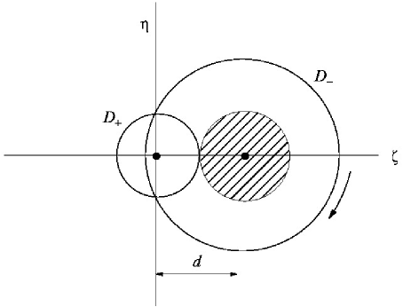
Figure 7: The rescaled oscillator phase plane showing the disks $D_{+}$ and $D_{-}$. The shaded region indicates those initial conditions in $D_{-}$ which never enter the intersection $S$ of $D_{-}$ and $D_{+}$, and thus lead to trajectories in which the particle remains in the interaction region. These trajectories make up what we have referred to as Void I, with the center of $D_{-}$ corresponding to the center of that elliptic island.

Note that in this essentially geometric description, the dynamics depends only on three independent parameters $E,L$, and $\alpha$. It is helpful to simplify the geometric nature of the description even further, by reorganizing the parameters as follows. First, we re-express the coupling strength of the system through the parameter

$$d=\frac{\alpha}{\sqrt{2E+\alpha^{2}}}$$ (12)

and introduce rescaled oscillator variables

$$\zeta=\frac{\Phi}{\sqrt{2E+\alpha^{2}}},\qquad\eta=\frac{\Pi}{\sqrt{2E+\alpha^{2}}}$$ (13)

which locate the oscillator phase point at radii

$$r_{\pm}=\frac{A_{\pm}}{\sqrt{2E+\alpha^{2}}},\qquad 0\leq r_{-}<1,\qquad 0\leq r_{+}<\sqrt{1-d^{2}}$$ (14)

from the centers, respectively, of a disk $D_{-}\$ of unit radius centered at $\left(d,0\right),$ and a disk $D_{+}$ of radius $\sqrt{1-d^{2}}$ centered at the origin. With this choice, the dynamics now occurs on the disks $D_{\pm},$ and the rotation angles $\varphi_{\pm}$ that the oscillator phase points sweep through during one traversal of the interaction zone can be simply written

$$\varphi_{-}\left(r_{-}\right)=\varphi_{-}\left(A_{-}\right)=\frac{a_{-}}{\sqrt{1-r_{-}^{2}}},\qquad a_{-}=\frac{2}{\sqrt{2E+\alpha^{2}}}$$ (15)

$$\varphi_{+}\left(r_{+}\right)=\varphi_{+}\left(A_{+}\right)=\frac{a_{+}}{\sqrt{1-d^{2}-r_{+}^{2}}},\qquad a_{+}=\frac{L}{\sqrt{2E+\alpha^{2}}}.$$ (16)

In this new description, we can thus take $d,$ $a_{+},$ and $a_{-}$ as the three independent parameters describing the system. Note that numerical data in the oscillator phase plots appearing throughout this paper are presented in terms of the scaled oscillator variables $\left(\zeta-d,\eta\right),$ and thus always appear on a disk of unit radius centered at the origin. This disk is essentially a shifted version of the disk $D_{-}\$defined above, but is rotated by 90 degrees, so that the oscillator coordinate appears on the vertical, rather than the horizontal axis. In what follows we will use both the scaled and unscaled variables as is appropriate to the discussion at hand.

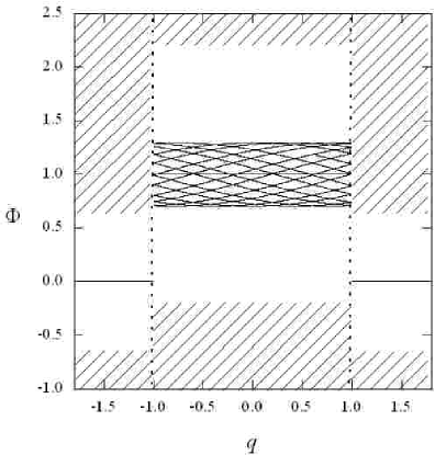
Figure 8: A partial trajectory in the $q-\Phi$ plane for a motion in which the particle remains confined to the interaction region. For this system $\alpha=1$ and $E=0.2$. Shaded portions indicate energetically inaccessible regions of configuration space for a system with this energy, and the region between the vertical dashed lines indicates the interaction region as described in the text.

V Motion Confined to the Interaction Region

In this section we analyze the motion of the system when the particle never leaves the interaction region. In particular, we explain the basic features of Void I, the region of complete integrability that occurs at the center of the phase space plots in Figs. 1(a) and (b), and in Fig. 4. In addition, we demonstrate and explain the existence of arcs of parabolic fixed points embedded in the chaotic regions of phase space.

The easiest case of confined motion to understand is the one in which the total energy is negative, and the particle is energetically confined to the interaction region. For this situation the dynamics is totally integrable, since the speed and kinetic energy of the particle are constants of the motion, and the oscillator coordinate $\Phi(t)$ is never negative. There are essentially three types of trajectories. The first type includes those in which only the motion of the particle is excited, so $\Phi=\alpha$ and $\Pi=0$ are constant. Since the particle does not have enough kinetic energy to overcome the barriers it encounters at $q=\pm 1,$ it reflects at each impact with the boundary. The trajectory is trivially periodic, with period $4/\dot{q}$. In the second type of motion, the particle is at rest in the interaction region and the oscillator performs simple harmonic motion of amplitude $\Phi_{0}<\alpha$ about $\Phi=\alpha.$ Periodic orbits of this type are also possible, of course, at any positive energy. Finally, there are confined motions in which both of the “modes” described above are excited. The trajectory is Lissajou-like, and the orbit is closed if the oscillator period and the traversal time $2/\dot{q}$ are commensurate. Otherwise it sweeps out a rectangle in the two-dimensional $\left(q,\Phi\right)$ configuration space, with $q\in\left[-1,1\right],$ and $\Phi\in\left[\alpha-\Phi_{0},\alpha+\Phi_{0}\right]$, for some positive amplitude $\Phi_{0}$ $<\alpha$ of oscillation.

When the total energy $E=0,$ possible motions with the particle confined to the interaction region include all of the types described above. In addition, oscillations of amplitude $\Phi_{0}=\alpha$ are now allowed; in that case the particle is at rest somewhere in the interaction region. We note that that the only other motions at $E=0$ are the unstable equilibrium points corresponding to the particle at rest outside the interaction region with the oscillator at rest as well.

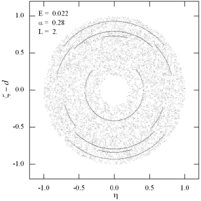
Figure 9: Phase plot showing arcs of periodic orbits. In this figure one can see a single arc of fixed points lying just outside of Void I, and, moving out from the center, sets of arcs corresponding to orbits of period $k=3,2,3,$ and $2$, corresponding, respectively, to $\ell=4,3,5$, and $5$.

We now give a description of all orbits at positive energy for which the particle never leaves the interaction zone. It is clear from Fig. 6 (a), the scaled version of which appears in Fig. 7, and the geometric description of Sec. III, that for any energy $\alpha^{2}/2>E>0,$ the disk $D_{+}$ does not contain the center of $D_{-}.$ Thus, for this situation, all initial conditions with $r_{-}<R_{\text{I}},$ indicated by the shaded region in Fig. 7, in which

$$R_{\text{I}}=d-\sqrt{1-d^{2}},$$ (17)

will give rise to trajectories for which the particle remains in the interaction region. Indeed, since the circle of radius $r_{-}$ does not then intersect $D_{+},$ successive rotations of such a point through $\varphi_{-}\left(r_{-}\right)$ can never lead to a point lying in $D_{+}.$ The elliptic regions of complete integrability at the center of Figs. 1(a) and (b), and in Fig. 4, which we have already referred to as Void I, correspond precisely to trajectories of this kind. In Fig. 8 we show a typical periodic orbit of this type in the $q-\Phi$ plane. Shaded portions of that figure indicate classically forbidden regions at this energy. From the equivalent point of view of a particle moving in a two dimensional potential $V\left(q,\Phi\right),$ it is interesting that the motion remains trapped within the interaction region although there is no actual potential energy barrier preventing it from leaving. Finally, we note that as $E$ is increased from zero at constant $\alpha$ the radius of Void I shrinks, as described by (17), until it finally disappears at the critical value $E=\alpha^{2}/2,$ (corresponding to $d=1/\sqrt{2}$), as in Fig. 1(c). For $E\leq 0$ Void I fills the entire oscillator phase space, as in Fig. 1(a).

Aside from these trajectories that remain within Void I, there are at any positive energy still other initial conditions that give rise to trajectories in which the particle remains in the interaction region. As we will show, however, such trajectories are then necessarily periodic. Indeed, suppose $r_{-}>d-\sqrt{1-d^{2}}.$ Then the circle of radius $r_{-}$ does necessarily intersect $D_{+},$ and successive rotations through $\varphi_{-}(r_{-})$ will take the orbit into $D_{+}$ whenever the rotation angle $\varphi_{-}(r_{-})$ is an irrational multiple of $2\pi$. Thus for the orbit to remain in $D_{-},$ it is necessary that the rotation angle $\varphi_{-}(r_{-})=2\pi\ell/k$ be rational, and hence that the orbit be periodic. Note that $k$ is then the period of the orbit (where it is understood that the integers $k$ and $\ell$ are relatively prime). Furthermore, for such a $k-$periodic orbit to be possible, the phase points must somehow arrange to miss the intersection with $D_{+}$ as they advance around $D_{-}\$in angular steps of $2\pi\ell/k.$ Clearly, for this to happen, the angle $\delta\left(r_{-}\right)$ subtended by the two intersection points of the edge of the disk $D_{+}$ and the circle of radius $r_{-}$ on which the phase point moves must be smaller than the angular separation between neighboring orbit points, i.e.,

$$\delta\left(r_{-}\right)<2\pi/k.$$

For fixed points $(k=1)$, this condition on the angle $\delta\left(r_{-}\right)$ is automatically satisfied, but for periodic orbits with $k\geq 2,$ the condition imposes a bound on $r_{-}$ that prevents, e.g., periodic orbits of this type occuring too close to the edge of $D_{-}.$

These arguments show that, in general, fixed points of the dynamics will occur at the radii

$$r_{\ell,-}=\sqrt{1-\left(\frac{a_{-}}{2\pi\ell}\right)^{2}}\qquad\ell>a_{-}/2\pi$$ (18)

for which $\varphi_{-}\left(r_{\ell,-}\right)=2\pi\ell.$ Note that this infinite sequence of values $r_{\ell,-}$ accumulates at $r_{-}=1,$ i.e., at the edge of $D_{-}.$ It follows that any phase point in $S_{\text{in }}=D_{-}(E)\setminus D_{+}(E)$ with $r_{-}=r_{\ell,-}$ will be a fixed point of the dynamics. The set of such points for a given value of $\ell$ is an arc in the phase plane. In Fig. 9, such an arc of fixed points with $\ell=1$ appears near the edge of Void I.

Now suppose for some value of $k>1$ and $r_{-}$ we have $\varphi_{-}\left(r_{-}\right)=2\pi\ell/k,$ and $\delta\left(r_{-}\right)<2\pi/k.$ In this situation there will exist $k$ arcs of angular span $2\pi/k-\delta\left(r_{-}\right)$ centered at $\left(d,0\right),$ each point of which is associated with a period $k$ orbit. Several arcs associated with higher order orbits of this type also appear in Fig. 9, and can occasionally be seen in some of our other phase plots. If the phase points were recorded at $q=\pm 1,$ then each arc that appeared in such a diagram would, by the arguments given above, lie outside of the intersection region with $D_{-}$, which is at the bottom of each phase diagram in this paper. However, because the phase points in these figures are recorded at $q=0$ when $p$ is positive, the angular position of each arc is rotated by an odd multiple of $\varphi_{-}\left(r_{-}\right)/2$ from where it would be if recorded at $q=\pm 1.$ This is due to the rotation of the oscillator phase point that occurs while the particle travels from the edge of the interaction region back to the center, where the phase point is recorded. Since this rotation is a function of the radius $r_{-}$, arcs of this kind can generally appear at any orientation in the phase diagram.

On general arguments it is to be expected that periodic trajectories of this kind are parabolic. Indeed, the stability matrix associated with a phase point lying on such an arc has a vanishing Lyapunov exponent along the direction tangent to the arc itself, since neighboring points along the arc are periodic orbits of the same order. On the other hand, in any neighborhood of such a point there will be initial conditions at radii $r_{-}$ just above or below the arc that will not satisfy (18) for any values of $\ell$ and $k$. Such points will give rise to trajectories in which the particle eventually does pass outside the interaction region, to end up at the mercy of the alternating shears $T_{+}$ and $T_{-}$, which give rise to the chaotic portions of the phase diagram. Thus, in general, we expect arcs of periodic trajectories of this type to be largely immersed in the chaotic parts of the phase diagram.

From the discussion above, which focuses on motions confined to the interaction region, one may wonder whether there are counterparts to these motions which take place with the particle confined entirely outside the interaction zone. In fact, it is easy to convince oneself that such motions are relatively few and far between. Indeed, for any point $X_{0}$ in $S_{\text{out}}$, the circle on which it moves necessarily intersects $D_{-}.$ Moreover, the angle $\delta_{+}\left(r_{+}\right)$ subtended by the two intersection points of the edge of the disk $D_{-}$ and the circle of radius $r_{+}$ on which the phase point moves is now greater than $\pi$. Hence, only period one orbits are able to avoid entering the interaction region. Such fixed points will occur whenever the time the particle takes to traverse the non-interaction region is an integer multiple of the oscillator period.

VI Other Periodic Orbits: Void II

Having thus classified all orbits in which the particle never leaves the interaction region, we now turn to the more complicated situation in which the particle explores the entire configuration space available to it. Of course, it is impossible to classify all such orbits, since they are precisely the ones that are responsible for the variety of intricate structures that appear, as well as for the chaos. Nonetheless, some of the more prominent features of our figures can be explained quantitatively. Indeed, we show in the analysis below that the fixed point at the centers of the elliptic islands that we have referred to as Void II arise from a relatively simple type of orbit in which the particle traverses each section of the ring exactly once per period. We also show that an infinite number of such fixed points exists, and that most of them are hyperbolic, and thus unstable.

Conceptually, such an orbit can be viewed within the geometric picture developed above, as follows. Consider a phase point $X_{0}$ on the $\zeta$-axis within $D_{-}$ at an instant when the particle is at the center of the interaction region and is moving to the right (See Fig. 10(a)). When the particle reaches $q=1,$ the oscillator phase point has rotated through an angle $\varphi_{-}\left(r_{-}\right)/2$ about the center of $D_{-}$ to the point $X_{1},$ as shown. The particle now leaves the interaction region and travels around the ring to $q=-1,$ while the oscillator phase point rotates through an angle $\varphi_{+}\left(r_{+}\right)$ to a point $X_{2}$. For the particle to now re-enter the interaction region, the point $X_{2}$ must lie in the intersection region $S$, as shown in Fig. 10(a). If, in addition, the system is to return to its original state $X_{0}$ when the particle arrives again at $q=0,$ it is obviously necessary for $X_{2}$ to fall on the circle of radius $r_{-}$ on which it started, as in Fig. 10(b). Thus, all periodic orbits that traverse each section of the ring exactly once per period have vertices $X_{1}$ and $X_{2}$ that lie on a “lozenge” structure of this type. Using relatively simple arguments, given below, we can locate the tops of all such lozenge orbits and demonstrate in the process that they are infinite in number.

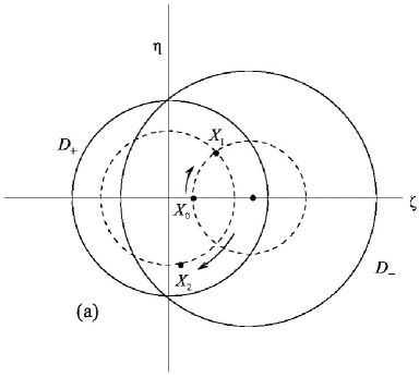
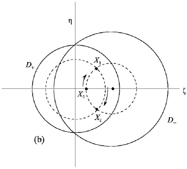
Figure 10: Motion on the disks $D_{-}$ and $D_{+}$, of lozenge orbits associated with fixed points of the dynamics.

To proceed, we recall that any point $X_{1}$ which forms the top or bottom of a lozenge orbit can be be obtained by rotating some point on the segment $\left(d-1,d+1\right)$ through an angle $\varphi_{-}\left(r_{-}\right)/2.$ The locus $\Gamma_{-}$ of all such points is depicted in Fig. 11 as a solid curve passing through the center of $D_{-}$. But any such point $X_{1}$ can also be obtained by rotating some point on the segment $\left(-\sqrt{1-d^{2}},\sqrt{1-d^{2}}\right)$ backwards in time through an angle $-\varphi_{+}\left(r_{+}\right)/2.$ The locus $\Gamma_{+}$ of this set of points is depicted as a solid line passing through the center of $D_{+}$ in the same figure. It should now be clear that the intersection points of these two curves locate all possible values $X_{1}$ associated with periodic orbits of this type. For each $X_{1}$ so located, the corresponding fixed point $X_{0}$ is obtained by rotating $X_{1}$ through $-\varphi_{-}\left(r_{-}\right)/2$. Since these two curves intersect an infinite number of times, the number of such fixed points is, itself, infinite. Indeed, the points $X_{1}^{\left(\infty\right)}$ and $X_{2}^{\left(\infty\right)}$ at the intersections of the edges of $D_{-}$ and $D_{+}$ are accumulation points of lozenge tips. In addition, any point where either of the two curves plotted in Fig. 11 crosses the edge of the disk in which it did not originate will also be an accumulation point of lozenge tips. As a result, it is clear that the points $X_{0\pm}^{\left(\infty\right)}$ with coordinates $\left(1\pm d,0\right)$ are accumulation points for fixed points of the dynamics. As we will show shortly, and as one might expect from the discussion of section IV, fixed points that occur too near the edge of either disk (where the shear strengths diverge) will be unstable.

On the other hand, the fixed points at the centers of the elliptic islands visible in Figs. 1(c)-(e), Figs. 2(a) and (c), Figs. 3(c), and Fig. 4(b) and (c) are clearly stable, and can therefore not be associated with an intersection of $\Gamma_{+}$ and $\Gamma_{-}$ that is too close to the edge of either disk. Based on this argument, the most reasonable candidate for such a fixed point is associated with the first intersection of $\Gamma_{+}$ and $\Gamma_{-}$ encountered when moving outward along $\Gamma_{+},$ starting from the origin. This intersection is readily computed numerically. For values of $E,L$, and $\alpha$ appropriate to our figures in which a Void II occurs, the results of such a calculation are tabulated in Table 1, and are indicated as horizontal dashed lines in the associated figures. To numerical accuracy the tabulated values agree with the actual locations of the centers of the type II Voids in those figures, supporting the basic picture developed above.

Let us now show how to predict in advance whether any particular intersection of $\Gamma_{+}$ and $\Gamma_{-}$ gives rise to a stable or unstable fixed point. To this end, it is clearly sufficient to consider the stability of the evolution in the neighborhood of the upper lozenge tip. Let $\vec{x}_{1}$ and $\vec{x}_{2}$ be the vectors, respectively, from the origin to the upper tip $X_{1}$, and to the lower tip $X_{2}$, of some lozenge, and let $\vec{x}_{i}^{\prime}=\vec{x}_{i}-\vec{d}$ be the corresponding vectors locating those points from the center of $D_{-}.$ By definition, $\vec{x}_{2}=T_{+}\vec{x}_{1}$, and $\vec{x}_{1}=T_{-}\vec{x}_{2},$ where $T_{+}$ and $T_{-}$ are the mappings associated with the evolution of the system during one traversal of the corresponding region by the particle. Note that $T_{-}T_{+}\vec{x}_{1}=\vec{x}_{1}$. It will therefore be sufficient to compute the Jacobian matrix of $T_{-}T_{+}$ at $X_{1}$. Because the points $X_{1}$ and $X_{2}$ are obtained from one another by moving along arcs of constant radius from the centers of $D_{\pm},$ it follows that $r_{\pm}\left(\vec{x}_{1}\right)=r_{\pm}\left(\vec{x}_{2}\right),$ $\varphi_{+}\left(\vec{x}_{1}\right)=\varphi_{+}\left(\vec{x}_{2}\right)$ $=\phi,$ and $\varphi_{-}\left(\vec{x}_{1}\right)=\varphi_{-}\left(\vec{x}_{2}\right)=\psi.$ Specifically, this means that

$$\vec{x}_{1}=\vec{d}+R\left(\psi\right)\left(\vec{x}_{2}-\vec{d}\right)=T_{-}\;\vec{x}_{2}\qquad\vec{x}_{2}=R\left(\phi\right)\;\vec{x}_{1}=T_{+}\vec{x}_{1}$$

where the rotation matrix

$$R\left(\theta\right)=\left(\begin{array}[]{cc}\cos\theta&\sin\theta\\ -\sin\theta&\cos\theta\end{array}\right)$$

induces a rotation in the clockwise sense through an angle $\theta$. We compute first the Jacobian matrix $J_{+}$ of $T_{+}$ at $X_{1}$

$$J_{+} =\left(\begin{array}[]{cc}\cos\phi&\sin\phi\\ -\sin\phi&\cos\phi\end{array}\right)+\frac{\phi^{\prime}}{r_{+}}\left(\begin{array}[]{cc}-\sin\phi&\cos\phi\\ -\cos\phi&-\sin\phi\end{array}\right)\left(\begin{array}[]{cc}x_{1}x_{1}&x_{1}y_{1}\\ x_{1}y_{1}&y_{1}y_{1}\end{array}\right)$$

$$=\left(\begin{array}[]{cc}\cos\phi&\sin\phi\\ -\sin\phi&\cos\phi\end{array}\right)-\frac{\phi^{\prime}}{r_{+}}\left(\begin{array}[]{cc}\cos\left(\phi-\pi/2\right)&\sin\left(\phi-\pi/2\right)\\ -\sin\left(\phi-\pi/2\right)&\cos\left(\phi-\pi/2\right)\end{array}\right)\left(\begin{array}[]{cc}x_{1}x_{1}&x_{1}y_{1}\\ x_{1}y_{1}&y_{1}y_{1}\end{array}\right)$$

$$=R\left(\phi\right)-r_{+}\phi^{\prime}R\left(\phi-\pi/2\right)\;\hat{x}_{1}\hat{x}_{1}$$

where $\hat{x}\hat{x}$ denotes the second rank tensor product of the unit vector $\hat{x}$ with itself. Similarly, we consider the Jacobian $J_{-}$ of $T_{-}$ at $X_{2}$

$$J_{-} =\left(\begin{array}[]{cc}\cos\psi&\sin\psi\\ -\sin\psi&\cos\psi\end{array}\right)+\frac{\psi^{\prime}}{r_{-}\left(\vec{x}_{2}\right)}\left(\begin{array}[]{cc}-\sin\psi&\cos\psi\\ -\cos\psi&-\sin\psi\end{array}\right)\left(\begin{array}[]{cc}x_{2}^{\prime}x_{2}^{\prime}&x_{2}^{\prime}y_{2}\\ x_{2}^{\prime}y_{2}&y_{2}^{\prime}y_{2}^{\prime}\end{array}\right)$$

$$=\left(\begin{array}[]{cc}\cos\psi&\sin\psi\\ -\sin\psi&\cos\psi\end{array}\right)-\frac{\psi^{\prime}}{r_{-}\left(\vec{x}_{2}\right)}\left(\begin{array}[]{cc}\cos\left(\psi-\pi/2\right)&\sin\left(\psi-\pi/2\right)\\ -\sin\left(\psi-\pi/2\right)&\cos\left(\psi-\pi/2\right)\end{array}\right)\left(\begin{array}[]{cc}x_{2}^{\prime}x_{2}^{\prime}&x_{2}^{\prime}y_{2}\\ x_{2}^{\prime}y_{2}&y_{2}^{\prime}y_{2}^{\prime}\end{array}\right)$$

$$=R\left(\psi\right)-r_{-}\psi^{\prime}R\left(\psi-\pi/2\right)\hat{x}_{2}^{\prime}\hat{x}_{2}^{\prime}.$$

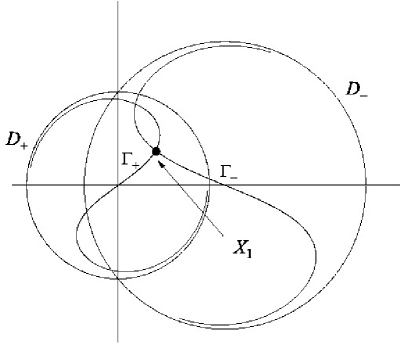
Figure 11: Intersection of the curves $\Gamma_{-}$ and $\Gamma_{+}$, described in the text, locating the tip $X_{1}$ of a lozenge orbit. Each curve wraps an infinite number of times around the edge of the disk in which it originates.

The trace of the product

$$J_{-}J_{+} =(R\left(\psi\right)-r_{-}\psi^{\prime}R\left(\psi-\pi/2\right)\hat{x}_{2}^{\prime}\hat{x}_{2}^{\prime})(R\left(\phi\right)-r_{+}\phi^{\prime}R\left(\phi-\pi/2\right)\;\hat{x}_{1}\hat{x}_{1})$$

$$=R\left(\phi+\psi\right)-r_{-}\psi^{\prime}R\left(\psi-\pi/2\right)\hat{x}_{2}^{\prime}\hat{x}_{2}^{\prime}R\left(\phi\right)-r_{+}\phi^{\prime}R\left(\psi+\phi-\pi/2\right)\;\hat{x}_{1}\hat{x}_{1}$$

$$\ \qquad\qquad\qquad\qquad\qquad+r_{-}r_{+}\psi^{\prime}\phi^{\prime}R\left(\psi-\pi/2\right)\hat{x}_{2}^{\prime}\hat{x}_{2}^{\prime}R\left(\phi-\pi/2\right)\;\hat{x}\hat{x}$$

of these two matrices determines the stability of the evolution in the neighborhood of the lozenge tip $X_{1}$ associated with the orbit. The trace of the first term is obvious. To evaluate the second, use $\text{Tr}\left[\vec{x}\vec{y}\right]=\vec{x}\cdot\vec{y},$ and the invariance of the trace of a product of operators under their cyclic permutation:

$$\text{Tr}R\left(\psi-\pi/2\right)\hat{x}_{2}^{\prime}\hat{x}_{2}^{\prime}R\left(\phi\right) =\text{Tr}R\left(\phi\right)R\left(\psi-\pi/2\right)\hat{x}_{2}^{\prime}\hat{x}_{2}^{\prime}=\text{Tr}\left(R\left(\phi+\psi-\pi/2\right)\hat{x}_{2}^{\prime}\right)\cdot\hat{x}_{2}^{\prime}$$

$$=\cos\left(\phi+\psi-\pi/2\right).$$

Similarly, $\text{Tr}\left[R\left(\psi+\phi-\pi/2\right)\;\hat{x}_{1}\hat{x}_{1}\right]=\cos\left(\phi+\psi-\pi/2\right).$ The trace of the last term similarly reduces to the product

$$\text{Tr}\left[R\left(\psi-\pi/2\right)\hat{x}_{2}^{\prime}\hat{x}_{2}^{\prime}\;R\left(\phi-\pi/2\right)\hat{x}_{1}\hat{x}_{1}\right] =\left(\hat{x}_{2}^{\prime}\cdot R\left(\phi-\pi/2\right)\hat{x}_{1}\right)\text{Tr}\left[R\left(\psi-\pi/2\right)\hat{x}_{2}^{\prime}\hat{x}_{1}\right]$$

$$=\left(\hat{x}_{2}^{\prime}\cdot\left[R\left(\phi-\pi/2\right)\hat{x}_{1}\right]\right)\left(\hat{x}_{1}\cdot\left[R\left(\psi-\pi/2\right)\hat{x}_{2}^{\prime}\right]\right).$$

To evaluate this we need to consider more carefully the geometry of the situation. Let $\theta_{-}=$ $\psi/2$ and $\theta_{+}=\phi/2\$be the interior angles adjacent to the base of the triangle connecting the centers of $D_{-}$ and $D_{+}$ to the point $X_{1}.$ Note that the sum $\theta_{+}+\theta_{-}\leq\pi$. The angle $\chi=\pi-\theta_{+}-\theta_{-}$ opposite this base is the angle between the vectors $\vec{x}_{1}$ and $\vec{x}_{1}-\vec{d}=\vec{x}_{1}^{\prime}.$ So

$$\hat{x}_{1}=R\left(\pi-\theta_{+}-\theta_{-}\right)\hat{x}_{1}^{\prime}.$$

But a vector along $\hat{x}_{2}^{\prime}$ is rotated into a vector along $\hat{x}_{1}^{\prime}$ by a rotation through $\phi=2\theta_{-},$ i.e., $\hat{x}_{1}^{\prime}=R\left(2\theta_{-}\right)\hat{x}_{2}^{\prime},$ so

$$\hat{x}_{1}=R\left(\pi-\theta_{+}-\theta_{-}\right)R\left(2\theta_{-}\right)\hat{x}_{2}^{\prime}=R\left(\pi-\theta_{+}+\theta_{-}\right)\hat{x}_{2}^{\prime}.$$

This leads to

$$\hat{x}_{1}\cdot\left[R\left(\psi-\pi/2\right)\hat{x}_{2}^{\prime}\right]=\hat{x}_{1}\cdot\left[R\left(\frac{\psi}{2}+\frac{\phi}{2}-3\pi/2\right)\hat{x}_{1}\right]=\cos\left(\frac{\psi}{2}+\frac{\phi}{2}-3\pi/2\right)=-\sin\left(\frac{\psi+\phi}{2}\right)$$

and

$$\hat{x}_{2}^{\prime}\cdot\left[R\left(\phi-\pi/2\right)\hat{x}_{1}\right] =\hat{x}_{2}^{\prime}\cdot\left[R\left(\phi-\pi/2\right)R\left(\pi-\theta_{+}+\theta_{-}\right)\hat{x}_{2}^{\prime}\right]=\hat{x}_{2}^{\prime}\cdot\left[R\left(\frac{\psi}{2}+\frac{\phi}{2}+\pi/2\right)\hat{x}_{2}^{\prime}\right]$$

$$=\cos\left(\frac{\psi}{2}+\frac{\phi}{2}+\pi/2\right)=-\sin\left(\frac{\psi+\phi}{2}\right).$$

Thus, for the lozenge evolution,

$$\text{Tr}\left[J_{-}J_{+}\right]=2\cos\left(\psi+\phi\right)-\left(r_{-}\psi^{\prime}+r_{+}\phi^{\prime}\right)\sin\left(\phi+\psi\right)+r_{-}r_{+}\psi^{\prime}\phi^{\prime}\sin^{2}\left(\frac{\psi+\phi}{2}\right)$$ (19)

or

$$\text{Tr}\left[J_{-}J_{+}\right]=2+\left(r_{-}r_{+}\psi^{\prime}\phi^{\prime}-4\right)\sin^{2}\left(\frac{\psi+\phi}{2}\right)-2\left(r_{-}\psi^{\prime}+r_{+}\phi^{\prime}\right)\sin\left(\frac{\psi+\phi}{2}\right)\cos\left(\frac{\psi+\phi}{2}\right).$$ (20)

From this form it is first of all possible to prove, confirming our previous arguments, that fixed points associated with lozenge tips close to the edge of either disk (where $\psi^{\prime}$ and $\phi^{\prime}$ diverge) are unstable. This is easily shown for $d<1/\sqrt{2}$. In that case, a little trigonometry shows that the angle $\chi$ associated with any lozenge tip near the boundary of $S$ is acute, so that $\pi\geq\left(\psi+\phi\right)/2>\pi/2.$ Consequently, $\text{Tr}\left[J_{-}J_{+}\right]\geq 2$, with equality only if $\sin\left(\psi+\phi\right)/2=0$, so that the fixed point is hyperbolic or, at worst, parabolic. For this last case to occur the angles $\psi/2$ and $\phi/2$ must add up to $\pi,$ which can only happen if $\Gamma_{+}$ and $\Gamma_{-}$ intersect on the horizontal axis. In that case, $\phi/2=\pi$ and $\psi/2=0,$ or vice versa. It is not hard to convince oneself that, for any fixed value of $d,$ there exist arbitrarily large values of $a_{-}$ and $a_{+}$ where such fixed points will appear. All other fixed point of this type with $d<1/\sqrt{2}$ are, however, hyperbolic.

Figure   $$\zeta_{0}-d$$   Tr

1(c)

1(d)

1(e)

2(a)

2(b)

2(b)

2(b)

2(c)

3(b)

3(c)

4(b)

4(c)

Table 1: Location and stability of some lozenge type fixed points $X_{0}=(\zeta_{0},\eta_{0})=(\zeta_{0},0)$ appearing in the figures indicated.

Using the algorithm described above we have calculated numerically the location and stability, as indicated by the value of $\text{Tr}\left[J_{-}J_{+}\right]$, for the first intersection of $\Gamma_{+}$ and $\Gamma_{-}$ for the system parameters of a certain number of our figures. The results appear in Table 1. Comparison with the relevant figures shows that whenever $|\text{Tr}\left[J_{-}J_{+}\right]|<2$ the associated fixed point is indeed the center of a Void II. For Fig. 3(b), this fixed point, computed to lie at $\zeta-d=-0.575$, has a trace with magnitude just greater than 2. It appears as the hyperbolic structure located below Void I in that figure. In Fig. 2(b), we have, in addition, computed the second and third intersection of $\Gamma_{+}$ and $\Gamma_{-}$. One leads to a fixed point at $\zeta-d=0.878$, which is stable, and appears at the center of a crescent shaped strucure at the top of that figure. The other occurs at $\zeta-d=-0.864$, but is unstable. It does not, therefore, give rise to an elliptic island, but lies right at the edge of Void II.

Finally, although in general the location of the fixed point at the center of Void II must be determined numerically, its behavior for large energy can be obtained from the limiting behavior of the dynamics as $d,$ $a_{+},$ and $a_{-}$ go to zero. In this limit, denoting the location of the fixed point as $X_{0}=\left(\eta d,0\right),$ we note that the curves $\Gamma_{\pm}$ are well represented by straight lines in the neighborhood of the origin. The corresponding triangle bounded by the segment $\left[0,d\right]$ and $\Gamma_{\pm}$ then has a height $h=\eta d\tan a_{+}\sim\eta da_{+}=\eta Ld^{2}/\alpha$ as measured from the origin, and $h=\left(1-\eta\right)d\tan a_{-}\sim\left(1-\eta\right)da_{-}=\left(1-\eta\right)d^{2}/\alpha$ as measured from $\left(d,0\right),$ so that

$$\eta d=\frac{2d}{2+L}$$ (21)

locates the corresponding fixed point on the segment $\left[0,d\right].$ This has a simple physical interpretation. At high energies, when the particle is moving very fast, the fractional change in its speed as it enters and exits the interaction region is small. In such a motion, the reduced oscillator coordinate oscillates about equilibrium position $d$ during that fraction $2/\left(2+L\right)$ of the time the particle is in the interaction region, and oscillates about the origin during that fraction $L/\left(2+L\right)$ of the time that the particle is outside the interaction region. A time average of these two values of the equilibrium position results in the location (21) of the fixed point in this high energy limit.

Having thus made our point that the most prominent features that appear in our phase plots can be explained in terms of the simplest periodic orbits of the system, we point out that many other periodic orbits occur in which the particle traverses the two sections of the ring more than once per period. Such orbits will then give rise to the more complicated structures appearing, e.g. in Fig. 5. We conjecture that a more complete analysis of those orbits along lines similar to those developed in this paper, would allow a complete explanation of some of the more anthropomorphic structures appearing in that figure.

VII Discussion and Summary

The model we have introduced and studied in this paper clearly has certain similarities to a number of previously studied dynamical systems, such as the kicked rotor, the Fermi accelerator, billiards, and the spring-pendulum. Indeed, the study of the dynamics reduces in all these cases to the study of a return map on a suitably chosen Poincaré section. The model presented here nevertheless differs in important ways from each of these previously studied systems.

Indeed, the kicked rotor and the Fermi accelerator describe externally perturbed nonconservative systems with one degree of freedom, while the current model is closed, energy-conserving, and has two degrees of freedom. In our model, although the particle gets “kicked” each time it reaches $q=\pm 1$, the kicks are neither periodic in time, as in the rotor, nor are they imposed by an external agent, as is the case for both the rotor and the Fermi accelerator.

Billiards, of course, are closed conservative systems with two degrees of freedom as well, but trajectories in billiards have the unusual property of being independent of particle energy, so that changing the energy does not change the statistical features of the dynamics. This is in sharp contrast to the behavior of the present model, in which many of the interesting features that arise, do so as a result of changes in the energy of the system under conditions in which the underlying potential is kept fixed. Moreover, the present system can be interpreted in terms of the Hamiltonian interaction between two otherwise separate mechanical systems. It should, therefore, be of more use in understanding many problems for which that is an essential feature.

Another closed Hamiltonian system of that type is the spring-pendulum Broer1 ; Broer2 . Like the current model, the spring-pendulum is a Hamiltonian system with two degrees of freedom, each of which has a simple description when treated on its own. Unlike the spring-pendulum, however, the present model has the advantage that the coupling between the two sub-systems can be smoothly turned off in a way that allows the unperturbed dynamics of each to be recovered, and thus may be more useful for understanding fundamental properties of interacting independent systems of this type. We note that a bifurcation analysis for the spring-pendulum was given in Broer2 . A similar analysis applied to our model would yield predictions on the motion and the shape of the elliptic islands that appear in our model as the parameters are changed, and could be an interesting direction for future study. Our emphasis here has instead been on some unusual features of our model, that we now briefly recall.

We have argued that for suitable system parameters the system exhibits either a fully chaotic phase space, or a mixed phase space in which only two regions occur. In one the motion is chaotic, and in the other it is completely integrable with no secondary KAM structures (See Fig. 1(b) and (c)). While we have explained the presence of chaos in the model in terms of alternating shears similar to the kind that arise in linked twist maps, our conjecture regarding the absence of secondary structures of finite measure in the chaotic sea for small energies is based largely on numerical calculations over very small regions of phase space that have heretofore failed to detect any structure in the chaotic region. We have not, however, given a rigorous proof that such structures do not emerge at small enough length scales in phase space.

We note also that the sharp boundary that exists in this model between the chaotic and the completely integrable parts of phase space should make it an interesting system on which to test current conjectures of quantum chaos theory, in particular those pertaining to systems with a mixed phase space, and to the localization properties of eigenfunctions on chaotic and completely integrable parts of phase space. While the clear-cut boundary of the present model should facilitate such an analysis, MP ; marklof it does have the complication of an underlying potential that has finite discontinuities in configuration space, and the matching problems that occur, in contrast, e.g., to billiard systems, for which a number of efficient numerical techniques have been developed for solving the corresponding Schrödinger equation baecker .

Our own interest in the present system arose originally from a fundamental interest in Hamiltonian models of transport and dissipation in deformable media. In many such systems, the medium through which a particular transport species moves can be modeled as an appropriate collection of harmonic oscillators. Among the many questions that arise in such extended systems is, e.g., to what extent the presence of microscopic chaos, or its absence, in the interaction of a particle with a single oscillator, manifests itself in the transport properties that emerge at long times after repeated interactions with many independent or mutually-coupled oscillators. We view the present analysis as a step towards answering this and other questions related to systems of this kind.

- (1) L. Bruneau and S. De Bièvre, Commun. Math. Phys. 229, 511 (2002); F. Castella, L. Erdös, F. Frommelt, and P.A. Markovich, J. Stat. Phys. 100, 543 (2000); A.O. Caldeira and A.J. Leggett, Annals of Phys. 149, 374 (1983); G.W. Ford, J.T. Lewis, and R.F. O’Connell, J. Stat. Phys. 53, 439 (1988); Phys. Rev. A 37, 4419 (1988).
- (2) T. Holstein, Ann. Phys. (N.Y.) 8, 343 (1959); D. Emin, Advances in Physics 22, 57 (1973);ibid. 24, 305 (1975).
- (3) V.M. Kenkre and T.S. Rahman, Phys. Lett. A 50A, 170 (1974); A.C. Scott, Phys. Rep. 217, 1 (1992); A.S. Davydov, Phys. Status Solidi 30, 357 (1969); A. C. Scott, P. S. Lomdahl, and J. C. Eilbeck, Chem. Phys. Lett. 113, 29 (1985); M. I. Molina and G. P. Tsironis, Physica D 65, 267 (1993); D. Hennig and B. Esser, Z. Phys. B 88, 231 (1992); V. M. Kenkre and D.K. Campbell, Phys. Rev. B 34, 4959 (1986); D.W. Brown, B.J. West, and K. Lindenberg, Phys. Rev. A 33, 4110 (1986); D.W. Brown, K. Lindenberg, and B.J. West, Phys. Rev. B 35, 6169 (1987); M.I. Salkola, A.R. Bishop, V. M. Kenkre, and S. Raghavan, Phys. Rev. B 52, 3824 (1995). V. M. Kenkre, S. Raghavan, A.R. Bishop, and M.I. Salkola, Phys. Rev. B 53, 5407 (1996).
- (4) V.M. Kenkre and L. Giuggioli, Chem. Phys. 296, 135 (2004), and references therein.
- (5) Other approaches aimed at understanding purely classical versions of the polaron problem, and which utilize Hamiltonians for interacting oscillators (with no itinerant particle, as studied here) reveal curious features in the dynamics. See. e.g., V.M. Kenkre, P. Grigolini, and D. Dunlap, “Excimers in Molecular Crystals”, in Davydov’s Soliton Revisited, P.L. Christiansen and A.C. Scott, eds., p. 457 (Plenum 1990); V.M. Kenkre and X. Fan, Z. Physik B 70, 233 (1988).
- (6) J. Malovrh and T. Prosen, J. Phys. A 35, 2483 (2002).
- (7) R. Burton and R.W. Easton, Global Theory of Dynamical Systems (Proc. Internat., Northwestern Univ., Evanston Ill., 1979), pp. 35-49, Lecture Notes in Mathematics 819 (Springer, Berlin 1980); F. Przytycki, Ann. Sci. Ecole Norm. Sup. 4, 345-354 (1983).
- (8) H.W. Broer, I. Hoveujn, G.A. Lunter, G. Vegter, Nonlinearity 11, 1569-1605 (1998).
- (9) H.W. Broer, G.A. Lunter, G. Vegter, Physica D 112, 64-80 (1998).
- (10) J. Marklof, S. O’Keefe and S. Zelditch, Weyl’s law and quantum ergodicity for maps with divided phase space, Nonlinearity 18, 277 (2005).
- (11) A. Bäcker, Numerical aspects of eigenvalue and eigenfunction computations for chaotic quantum systems, in The Mathematical Aspects of Quantum Maps, M. Degli and S. Graffi (Eds.), Springer Lecture Notes in Physics 618, 91 (2003).