Forecasting non-stationary financial time series through genetic algorithm

Abstract

We utilize a recently developed genetic algorithm, in conjunction with discrete wavelets, for carrying out successful forecasts of the trend in financial time series, that includes the NASDAQ composite index. Discrete wavelets isolate the local, small scale variations in these non-stationary time series, after which the genetic algorithm’s predictions are found to be quite accurate. The power law behavior in Fourier domain reveals an underlying self-affine dynamical behavior, well captured by the algorithm, in the form of an analytic equation. Remarkably, the same equation captures the trend of the Bombay stock exchange composite index quite well.

It is well-known that a time series, which looks random in nature, may in fact be the outcome of a nonlinear deterministic but chaotic dynamics involving a few degrees of freedom. In such cases, it is possible to exploit this determinism to make short-term forecasts. Financial time series, originating from complex dynamical processes, are known to exhibit different types of behavior at different time scales ramsey ; mcaul ; bisw . Random processes like geometric Brownian motion mankiw and fractional Brownian motion mandel have been invoked for modelling stock market behavior. Fluctuations in the asset prices have also been analyzed through Levy-stable non-Gaussian model schu , a mixture of Gaussian distributions clark , etc. Separation of the fluctuations at short time scales, owing their origin to random processes, is essential before attempting any forecast, based on deterministic dynamics. This is made complicated due to the fact that, stock market composite indices often show non-stationary behavior bouch ; kantel . Wavelets, because of their multi-resolution capability and time-frequency localization are ideal to separate out the fluctuations at different time scales in non-stationary time series maran .

The goal of the present paper is to make use of discrete wavelets to isolate the fluctuations, at different scales, in non-stationary financial time series data and subsequently employ a recently developed genetic algorithm for short-term predictions of the trend szp ; alva ; kisht . We have used NASDAQ and Bombay Stock Exchange (BSE) composite indices for the purpose of our analysis.

We begin our work with reconstruction of dynamics in phase space from a time series. Theoretical ideas underlying this reconstruction are by now well-known and contained in the works of Ruelle ruel , Packard et al. packard , and Takens takens . Thus, given a deterministic time series $x(t_{k}),t_{k}=k\Delta t,k=1,...,N$, there exists a smooth map P satisfying

$$x(t)=P\left[x(t-\Delta t),x(t-2\Delta t),...,x(t-\emph{m}\Delta t)\right],$$ (1)

where m is called the embedding dimension and $\Delta t$ is the sampling time interval.

A genetic algorithm tries to obtain the function P, that best represents the map of a chaotic or integrable time series. The map can then be used to predict the future state of the system.

Genetic Algorithm.— The genetic algorithm considers an initial population of potential solutions consisting of elementary equation strings. These equation strings (individual solutions) are of the type as given in Eq.(1). Their right hand sides are stored in the computer as sets of character strings that contain random sequences of the variable at previous times, the four basic arithmetic symbols (+, -, X, and /), and real number constants. A criterion that measures how well the equation strings perform on a training set of the data is its fitness to the data, defined in Eq.(3) in the text. The strongest strings choose a mate for reproduction whereas the weaker strings become extinct. The newly generated population is subjected to mutations that change fractions of information. The evolutionary steps are repeated with the new generation. The process ends after a number of generation apriori defined by the user.

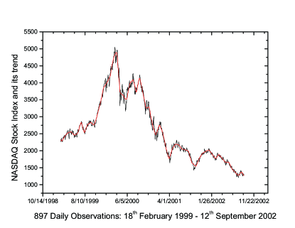
This technique is first applied to the time series of the NASDAQ composite index, in the region which shows maximum activity (897 points corresponding to the period between $18^{th}$ February 1999 to $12^{th}$ September 2002). A population consisting of 200 members was subjected to the iterative algorithm for carrying out one day ahead forecast. However, it was found that the forecast obtained from genetic algorithm was only marginally better than persistence forecast, $x_{t+1}=x_{t}$. It was thus felt that it would be better if one attempts to forecast the trend of the data, after removal of small-scale fluctuations, which owe their origin to random processes.

Figure 1: (Color Online) NASDAQ composite index (black line) and the trend extracted through Coiflets (red line) superimposed over it. The near matching of the two demonstrates the superb ability of the Coiflets in extracting the trend.

Extraction of trend through discrete wavelets.— For this purpose, we make use of Coiflets, a family of discrete wavelets, known to be ideally suited for capturing the trend in a data set daub . Discrete wavelets provide a complete orthonormal basis, which separates out the average (low-pass) part of a signal from the variations (high-pass). The orthonormal basis consists of scaling function (father wavelet) and mother and daughter wavelets. The scaling function finds out the trend in a data set, whereas the wavelets identify the variations at different scales. This is possible since the wavelets have multi-resolution abilities. Coiflets are compactly supported, with filter length 6N, where N is the order of the wavelet. These are nearly symmetrical and hence introduce minimal distortion while capturing the trend. Father function has 2N-1 vanishing moments, while mother and daughter wavelet functions have 2N vanishing moments; this endows them with the property of picking out the trend in an ideal manner.

The time series of the trend was subjected to the genetic algorithm. The first 700 points were used for training the algorithm and the remaining points were used for forecast verification. The genetic evolution process was initiated with 200 randomly selected equation strings, with m set to 4. m was found through false nearest neighbor approach that yielded the value of embedding dimension as 4 abarbanel . It was found that 5000 iterations were needed for extracting the forecast equation from the set. Interestingly, the analytic expression involves only three out of the four input parameters:

$$x_{fit}(t) = P_{fit}\left[x(t-1),x(t-3),x(t-4)\right]$$ (2)

$$= \frac{x(t-4)*(x(t-1))^{2}}{(x(t-3))^{2}}.$$

Note that $x_{fit}(t)$ is the prediction of $t^{th}$ day and $x(t-1),x(t-3)$ and $x(t-4)$ are the trends on the $(t-1),(t-3)$ and $(t-4)$ days respectively.

The above number of iterations were sufficient in the sense that increasing the number of iterations did not lead to a significant increase in the fitness strength:

$$R^{2}=1-\left[\frac{\Delta^{2}}{\sum(x_{0}-\langle x_{0}\rangle)^{2}}\right]$$ (3)

where, $\Delta^{2}=\sum(x_{c}-x_{0})^{2}$, $x_{c}$ is a parameter value estimated by the best scoring equation, $x_{0}$ is the corresponding ”true” value, $\langle x_{0}\rangle$ is the mean of the ”true” values of x.

In Fig.11, we show the time series of the data and the trend extracted through Coiflets-2, after removal of four level of high-pass coefficients. Retaining a few dominant high-pass coefficients, through other thresholding approaches like Donoho, did not have a significant effect here. More level of decomposition and thresholding was found to be detrimental to the prediction, since the same removes significant physical variations from the data set.

Figure 2: (Color Online) A zoomed portion of the NASDAQ composite index trend superimposed on predicted trend. Here the black line represents actual trend and the red circle symbol the predicted trend.

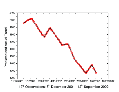
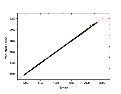
Next we made predictions for 747 (out of sample) points which were not used in training. It is worth pointing out that, since the embedding dimension m=4, we are left with 743 input-output relations. A zoomed portion of the same is depicted in Fig.2. Fig.3 shows the scatter plot of the predicted and actual trend, corresponding to time period between $30^{th}$ November 2001 to $17^{th}$ November 2004, showing a perfect fit. The equation of the best-fit straight line is, $y=1.00039x-0.59235$ and the coefficient of determination (square of the coefficient of correlation) was found to be 0.99994, signifying a high degree of correlation.

The efficacy of the prediction is further illustrated by the mean error through the average of modulus of return (in percent) which is found to be 0.06831 percent. Considering the fact that the signature of the trend (rise or fall) is of significance for financial time series we have further calculated the following quantity: $sign(x_{i+1}-x_{i})*sign(y_{i+1}-y_{i})$ where, $i$ goes from 1 to 742. The rise and fall are very well captured by the prediction equation (Eq.(2)), since the number of mismatches are only 40 out of 742.

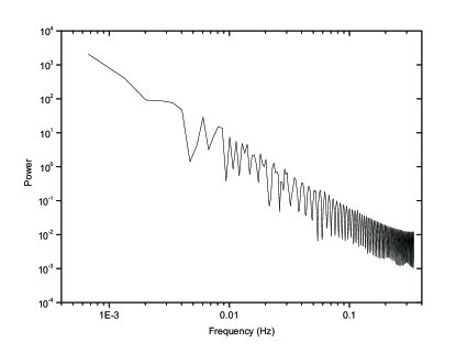
Self-similar dynamics of financial time series.— We have analyzed power spectrum of the trend, to ascertain the nature of this dynamical system and efficacy of the wavelets in removing small scale fluctuations. It is found that, the power spectrum shows self-similar behavior; the dynamics have both integrable and chaotic components. As seen in Fig.44, the power spectrum of Fourier transform of the trend has a power law decay with exponent 1.88. It has been recently shown that the corresponding exponent for chaotic dynamics is one, whereas the integrable systems have an exponent two rel1 ; rel2 ; santh . Hence, the trend of stock market dynamics in the present case is closer to an integrable system.

Figure 3: (Color Online) The scatter plot of the predicted and actual trend shows a linear behavior, illustrating the efficacy of the algorithm. Plus symbol represents scatter plot of the above, red line represents its linear fitting.

Figure 4: Power spectrum of the Fourier transform of the trend, in a log-log scale. Linear fit ($y=-1.88043x-4.26722$) indicates the closeness of the dynamics to integrable systems, for which the slope is -2.

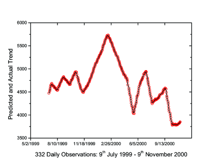
We have further checked the ability of the present algorithm using average of daily closing prices of BSE 30 index. This consists of 30 blue chip companies traded on the Bombay Stock Exchange. The compilation of the values is based on the ’weighted aggregates’ method. It is remarkable that the same equation for the trend as in Eq.(2) fits the trend of the BSE index, extracted through Coiflets, extremely well, as seen in Fig.5. This indicates the underlying similarity between the dynamical processes governing both the composite indices. The mean error found in prediction of BSE index was 0.08693 percent.

Figure 5: (Color Online) A zoomed portion of BSE Sensex trend and its prediction. Black line represents trend, red circle symbol represents the predicted trend.

In conclusion, a technique has been developed for predicting NASDAQ and other composite indices’ trend using the modern powerful genetic algorithm and discrete wavelet transform. The algorithm uses the past values of the trend extracted through wavelets for carrying out the prediction and is based on the Darwinian theory of survival of the fittest equation strings. The major advantage of using genetic algorithm versus other nonlinear forecasting techniques like neural networks is that an explicit analytic expression for the dynamic evolution of the trend in the time series is obtained.

It is quite possible that the technique will prove to be successful in forecasting the trend of individual stocks. The fluctuation in financial time series also show power law behavior indicating self similar nature gaba ; chak , it would be worthwhile to study their characteristic through this formalism. The fluctuations at very small scale, will not be amenable for modeling because of their random origin. Making use of wavelets, one can separate fluctuations at higher scales for the possibility of prediction. Work in these directions are in progress and will be reported in future.

The authors are indebted to Dr. A. Alvarez for generously providing the computer code of genetic algorithm used in the study.

References

- (1) J. B. Ramsey, D. Usikov and G. Zaslavsky, Fractals, 3, 2, 377 (1995).
- (2) J. L. McCauley, Dynamics of Markets (Cambridge University Press, Cambridge, 2004).
- (3) P. C. Biswal, B. Kamaiah and P. K. Panigrahi, J. Quant. Eco. 2, 133 (2004).
- (4) N. G. Mankiw, D. H. Romer and M. D. Shapiro, Rev. Eco. Stud., 58, 455 (1991).
- (5) B. B. Mandelbrot, Fractals and Scaling in Finance: Discontinuity, Concentration, Risk, (Springer-Verlag, 1997).
- (6) M. Schulz, S. Trimper and B. Schulz, Phys. Rev. E, 64, 026104-1:026104-5 (2001).
- (7) P. K. Clark, Econometrica, 41, 135 (1973).
- (8) J. P. Bouchaud, M. Potters and M. Meyer, Europhys. J., B 13, 595 (2000).
- (9) J. W. Kantelhardt, S. A. Zschiegner, E. Koscielny-Bunde, A. Bunde, S. Havlin and H. E. Stanley, Physica A, 316, 87 (2002).
- (10) P. Manimaran, P. K. Panigrahi and J. C. Parikh, arXiv:nlin.CD/0412046.
- (11) G. G. Szpiro, Phys. Rev. E 55, 257 (1997).
- (12) A. Alvarez, C. Lopez, M. Riera, E. Henandez-Garcia and J. Tintore, Geophys. Res. Lett. 27, 2709 (2000).
- (13) C. M. Kishtawal, S. Basu, F. Patadia, and P. K. Thapliyal, Geophys. Res. Lett. 30, 2203 (2003).
- (14) D. Ruelle, Ergodic theory of differentiable dynamical systems. Publ. Math. IHES 50, 27 (1979).
- (15) N. H. Packard, J. P. Crutchfield, J. D. Farmer and R. S. Shaw, Phys. Rev. Lett., 45, 712 (1980) 87
- (16) F. Takens, in Dynamical Systems and Turbulence, edited by D. A. Rand and L. L. Young, Lecture Notes in Mathematics Vol. 898 (Springer Verlag, Berlin, 1981).
- (17) I. Daubechies, Ten Lectures on Wavelets (SIAM, Philadelphia, 1992).
- (18) H. Abarbanel, R. Brown, J. Sidorovich and L. Tsimring, Rev. of Mod. Phys., 65, 1331 (1993).
- (19) A. Relao, J. M. G. Gmez, R. A. Molina, and J. Retamosa, Phys. Rev. Lett. 89, 244102 (2002).
- (20) A. Relao, R. A. Molina, and J. Retamosa, Phys. Rev. E 70, 017201 (2004).
- (21) M. S. Santhanam and J. N. Bandyopadhyay, arXiv:nlin.CD/0502007.
- (22) X. Gabaix, P. Gopikrishnan, V. Plerou and H. E. Stanley, MIT Dept. Eco. Working Paper No. 03-30 (2003).
- (23) A. Chakraborti and M. S. Santhanam, accepted for publication in Int. J. Mod. Phys. C (2005).