Finite-size effects on open chaotic advection

Abstract

We study the effects of finite-sizeness on small, neutrally buoyant, spherical particles advected by open chaotic flows. We show that, when projected onto configuration space, the advected finite-size particles disperse about the unstable manifold of the chaotic saddle that governs the passive advection. Using a discrete-time system for the dynamics, we obtain an expression predicting the dispersion of the finite-size particles in terms of their Stokes parameter at the onset of the finite-sizeness induced dispersion. We test our theory in a system derived from a flow and find remarkable agreement between our expression and the numerically measured dispersion.

I Introduction

A proper understanding of chaotic advection aref1 in incompressible, open flows is substantially relevant, as applications range from laboratory experiments horner1 to environmental flows of oceanographic abraham1 and atmospherical importance koh1 . Usually, open flows displaying chaotic advection are asymptotically regular, but the dynamics of the advected particles possesses a chaotic saddle kantz1 which governs the transient behavior of the orbits. This saddle is an invariant set consisting of infinitely many unstable orbits organized in a fractal structure. Its stable and unstable manifolds also display fractality and can be observed directly in physical space. In particular, the unstable manifold is traced out by an ensemble of fluid particles initially placed in the region of the saddle.

The fundamental aspects of chaotic advection in open flows are now relatively well known (see karolyi1 and references therein), but almost exclusively in the case where the particles are considered to move as fluid particles (passive tracers), without inertia. This situation is termed passive advection. In many important flows, however, the finite-sizeness of the particles has to be considered balkovsky1 . The resulting dynamics is strikingly different from passive advection. In particular, the phase space for finite-size particles has twice the number of dimensions of the phase space of passive advection. The latter is simply the configuration space (physical space), and corresponds to an invariant subspace of the former. The higher dimensionality results from the new degrees of freedom corresponding to the components of the velocity of the finite-size particles. This is a consequence of the fact that the finite-size particles are not constrained to have the velocity of the advected fluid. By contrast, the velocities of passive tracers do coincide with the velocity of the flow.

One consequence of this difference is that the motion of finite-size particles can diverge from the motion of the corresponding passive tracers in certain regions of the flow, even when the particles have the same density as the fluid babiano1 . We stress that this divergence arises solely from the finite-size character of the particles, which we consider here to be neutrally buoyant benczik1 , i.e., they have the same density as the fluid. The aim of this paper is to investigate the consequences of this divergence to open chaotic advection. We argue and show that, when projected onto the configuration space, the advected finite-size particles disperse about the chaotic saddle (and its unstable manifold) corresponding to passive advection. This is a general phenomenon that had not been reported so far. We develop a theory to analyze it. We obtain a quantitative expression for the dispersion of the finite-size particles about the chaotic saddle and its unstable manifold in configuration space as a function of the Stokes parameter. We test and validate our theory using the blinking vortex-source system and find a strikingly good agreement with the directly measured dispersion. A major consequence of this dispersion is that finite-size effects can destroy the fractal structure of open chaotic advection in configuration space, with severe consequences to active flows toroczkai1 ; nishikawa1 .

II Continuous description of the dynamics

In dimensionless form, the equation of motion for a small rigid spherical particle advected by an incompressible fluid of same density with a given velocity field ${\bf u}({\bf r},t)$ is maxey1

$$\frac{d{\bf v}}{dt}=\frac{D{\bf u}}{Dt}-\frac{1}{\mbox{St}}\left({\bf v}-{\bf u}\right)-\frac{1}{2}\left(\frac{d{\bf v}}{dt}-\frac{D{\bf u}}{Dt}\right),$$ (1)

where ${\bf v}$ is the velocity of the particle and $\mbox{St}=\frac{2a^{2}U}{9\nu L}$ is its Stokes number. Here $a$ is the radius of the particle, whereas $U$ and $L$ are the characteristic velocity and lenght of the flow, respectively. The kinematic viscosity of the fluid is given by $\nu$. Physically, the Stokes number is a measure of the finite-size effects. In the limit of vanishing Stokes number, we recover passive advection, with ${\bf v}={\bf u}$. Equation (1) is Newton’s law with the terms on the right hand side corresponding, respectively, to the force exerted by the undisturbed flow, Stokes drag and the added-mass effect. In this approximation, the Faxén corrections and the Basset-Boussinesq history force term are neglected maxey1 .

If we write the derivative along the trajectory of the fluid element, $\frac{D{\bf u}}{Dt}=\frac{\partial{\bf u}}{\partial t}+({\bf u}\cdot\nabla){\bf u}$, in terms of the derivative along the trajectory of the particle, $\frac{d{\bf u}}{dt}=\frac{\partial{\bf u}}{\partial t}+({\bf v}\cdot\nabla){\bf u}$, we cast Eq. (1) into the form babiano1

$$\frac{d{\bf A}}{dt}=-\left(\mathsf{J}_{\bf u}+\frac{2}{3\mbox{ St}}\mathbbm{1}\right)\cdot{\bf A},$$ (2)

where ${\bf A}={\bf v}-{\bf u}$ and $\mathsf{J}_{\bf u}$ is the Jacobian of ${\bf u}$. For convenience, we treat a two-dimensional fluid flow, so the dynamics of finite-size particles occurs in a $4$-dimensional phase space. The configuration space, corresponding to ${\bf A}={\bf 0}$, is a $2$-dimensional invariant subspace where passive advection takes place.

III The open flow model

In order to illustrate the finite-size effects in open chaotic advection, we choose the blinking vortex-source system for the flow karolyi1 ; aref2 . This system is periodic and consists of two alternately open point sources in a plane. It models the alternate injection of rotating fluid in a large shallow basin. Apart from the two point sources, the dynamics is Hamiltonian, with the streamfunction given by $\Psi=-\left(K\ln r^{\prime}+Q\phi^{\prime}\right)\Theta(\tau)-\left(K\ln r^{\prime\prime}+Q\phi^{\prime\prime}\right)\Theta(-\tau)$, where $\tau=0.5T-t\mbox{ mod }T$. Here, $r^{\prime}$ and $\phi^{\prime}$ are polar coordinates centered at $(-1,0)$ whereas $r^{\prime\prime}$ and $\phi^{\prime\prime}$ are polar coordinates centered at $(1,0)$. The two parameters $Q$ and $K$ are, respectively, the strenghts of the source and of the vortex. The period of the flow is $T$, whereas $\Theta$ stands for the Heaviside step function. The sources are located at positions $(\pm 1,0)$. For each half period, the system remains stationary with only one of the sources open. This allows one to analytically integrate the equations of motion, $u_{x}=\partial\Psi/\partial y$ and $u_{y}=-\partial\Psi/\partial x$, during each half period, and thus to write explicitly a stroboscopic map for this system, recording the positions of the particles after integer multiples of the period $T$. In complex representation, $z=x+iy=r\mbox{ exp}(i\phi)$, the stroboscopic map is

$$z_{n+1}=\left(z^{\prime}_{n}-1\right)\left(1-\frac{\eta}{|z^{\prime}_{n}-1|^{2}}\right)^{1/2-i\xi/2}+1,$$ (3)

where $z^{\prime}_{n}=\left(z_{n}+1\right)(1-\frac{\eta}{|z_{n}+1|^{2}})^{1/2-i\xi/2}-1,$ and where the two parameters governing the dynamics are $\eta\equiv QT$ and $\xi\equiv K/Q$. We fix $\eta=-0.5$ and $\xi=10$, for which the dynamics is chaotic. Figure 1(a) shows the unstable manifold of the chaotic saddle for passive tracers.

IV Discrete description of the dynamics

Equation (3) is the discrete version of the flow whose streamfunction is $\Psi$. Thus, passive advection is described by the two-dimensional area preserving map ${\bf x}_{n+1}={\bf f}({\bf x}_{n})$, in our case the one given by Eq. (3) with ${\bf x}_{n}$ written in complex representation as $z_{n}$. Analogously, a discrete version of Eq. (2) for the dynamics of finite-size particles is given by cartwright1

$${\bf x}_{n+2}-{\bf f}({\bf x}_{n+1})=\mbox{e}^{-\gamma}\mathsf{J}_{\bf f}({\bf x}_{n})\left({\bf x}_{n+1}-{\bf f}({\bf x}_{n})\right).$$ (4)

Equation (4) contains all the essential features of the flow given by Eq. (2). In particular, both have constant rate of phase space contraction. The term $-(\mathsf{J}_{\bf u}+\frac{2}{3\mbox{ St}}\mathbbm{1})$ in Eq. (2) is substituted by the expected term $\mbox{e}^{-\gamma}\mathsf{J}_{\bf f}({\bf x}_{n})$ in the map. The number $e^{-\gamma}$ plays the role of the Stokes parameter in the discrete dynamics. Equation (4) has been successfully used in the study of the dynamics of neutrally buoyant finite-size particles under chaotic advection cartwright2 and it was generalized in order to describe also the dynamics of particles whose density differs from that of the fluid motter1 . It is convenient to cast Eq. (4) into

$$\left\{\begin{array}[]{l}{\bf x}_{n+1}={\bf f}({\bf x}_{n})+{\bf w}_{n},\\[8.5359pt] {\bf w}_{n+1}=\mbox{e}^{-\gamma}\mathsf{J}_{\bf f}({\bf x}_{n}){\bf w}_{n}.\end{array}\right.$$ (5)

If $\lambda_{\bf x}$ and $\lambda_{\bf x}^{-1}$ are the eigenvalues of $\mathsf{J}_{\bf f}({\bf x})$, the vector ${\bf w}_{n}={\bf x}_{n+1}-{\bf f}({\bf x}_{n})$ is amplified in regions where $\gamma<|\ln|\lambda_{\bf x}||$. This corresponds to regions of the flow characterized by larger strain. In open chaotic flows with asymptotic regularity, such regions are precisely where the chaotic saddle is located. Consequently, there the finite-size particles may detach from their corresponding fluid elements and it is where the finite-size effects are expected to occur.

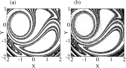
Figure 1: (a) Unstable manifold of the chaotic saddle. (b) The projection onto configuration space of the seventh iteration of Eq. (5) for an ensemble of particles with $\mbox{e}^{-\gamma}=0.2$. Initially, $10^{6}$ particles are uniformly distributed in the hypercube $[-0.5,0.5]\times[-1,0]\times[-10^{-3},10^{-3}]\times[-10^{-3},10^{-3}]\subset\mathbb{R}^{4}$. We plot only the region $[-2,2]\times[-2,1]$, where about $9\times 10^{4}$ are mapped to.

V Dispersion of the ensemble of finite-size particles

Analogously to the continuous case, the dynamics described by Eq. (5) takes place in a $4$-dimensional phase space. The configuration space corresponds to the $2$-dimensional invariant subspace ${\bf w}={\bf 0}$, where passive advection occurs. The limit of vanishing particle size corresponds to $\mbox{St}\rightarrow 0$ in the flow and to $e^{-\gamma}\rightarrow 0$ in the map. The solutions in this case are, respectively, ${\bf v}={\bf u}$ and ${\bf x}_{n+1}={\bf f}({\bf x}_{n})$. In this limit, we recover the motion of passive advection and an ensemble of particles initially located in the region of the chaotic saddle traces asymptotically its unstable manifold in the configuration space. As the size of the particles grows from zero, however, the particles trace out the unstable manifold in the $4$-dimensional phase space. The key point is that, when projected onto the configuration space, they do not trace the unstable manifold, $W^{u}(\Sigma)$, corresponding to passive advection, but they instead “disperse” about it. Figure 1(b) shows the projection onto the $2$-dimensional configuration space of the seventh iteration of an ensemble of finite-size particles, initially placed in the region of the chaotic saddle in the $4$-dimensional phase space. We thus have a clear qualitative picture of the finite-size effects, in which the smearing of the fractal structure in configuration space is evident. As the size of the particles gets larger, their “dispersion” about $W^{u}(\Sigma)$ increases.

VI Theory for the dispersion

To obtain a quantitative description of the phenomenon, we define the dispersion $D$ of a set $S_{1}$ about a set $S_{2}$ as the average of the distances $d(x,S_{2})$ between the points $x\in S_{1}$ and the set $S_{2}$. So we have

$$D=\langle d(x,S_{2})\rangle_{x\in S_{1}},$$ (6)

where $d(x,S_{2})=\mbox{min}\{d(x,y),y\in S_{2}\}$. Our goal is the derivation of an expression predicting the behaviour of the dispersion, about $W^{u}(\Sigma)$, of the position vectors in configuration space of an ensemble of finite-size particles whose initial conditions are $({\bf x}_{0},{\bf w}_{0})$, as a function of $\mbox{e}^{-\gamma}$. Differently from the case illustrated in Fig. 1(b), the initial positions ${\bf x}_{0}$ are chosen in the chaotic saddle, $\Sigma$, as our aim is to make a theory on the invariant set. Figure 2 shows the chaotic saddle. It is carefully obtained to warrant the correct natural measure jacobs1 . The initial conditions ${\bf w}_{0}$ are chosen so that $\|{\bf w}_{0}\|\ll 1$, corresponding to ${\bf v}\simeq{\bf u}$ in the flow, a condition assumed in the derivation of Eq. (1). The directions of the vectors ${\bf w}_{0}$ are randomly chosen with uniform angular distribution. We calculate the dispersion for the second iterate of the map, as this is the lowest iterate where the finite-size effects are present. The first iterate of the map, ${\bf x}_{1}$, is $\|{\bf w}_{0}\|$-distant from ${\bf f}({\bf x}_{0})$, independently of ${\mbox{e}}^{-\gamma}$, as we can see readily from Eq. (5). Figure 3 illustrates the situation that we aim to quantify.

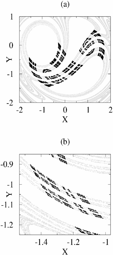
Figure 2: (a) The chaotic saddle (black) and its unstable manifold (grey). (b) Magnification of (a).

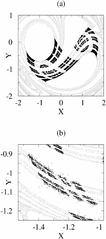
Figure 3: (a) The projection onto configuration space of the second iteration of Eq. (5) for an ensemble of particles with $\mbox{e}^{-\gamma}=0.2$. Initially, $6\times 10^{4}$ particles (black points) are placed in the chaotic saddle and the initial vectors ${\bf w}_{0}$ are uniformly chosen in the range $0<\|{\bf w}_{0}\|<10^{-3}$, and with uniform angular distribution. The unstable manifold $W^{u}(\Sigma)$ is also shown (grey points). (b) Magnification of (a).

In order to obtain the dispersion $D$ of the ensemble of finite-size particles about $W^{u}(\Sigma)$, we follow two steps. First, we derive an expression for the expected value, over both the natural measure of the chaotic saddle and the distribution of the initial vectors ${\bf w}_{0}$, of the distance between ${\bf x}_{2}$ and the unstable subspace arising from ${\bf f}^{2}({\bf x}_{0})$. This expected value $\delta_{\gamma}$ depends on the Stokes parameter $\mbox{e}^{-\gamma}$. The derivation of $\delta_{\gamma}$ involves only dynamical arguments. Second, we derive an expression for $D$ as a function of $\delta_{\gamma}$. This expression is necessary because the value of $D$ is smaller than $\delta_{\gamma}$. $W^{u}(\Sigma)$ is a fractal set and usually contains curves whose expected distance to the vector positions of the finite-size particles is smaller than $\delta_{\gamma}$. The situation is sketched in Fig. 4. Accordingly, the correct value of the dispersion $D$ of the finite-size particles about $W^{u}(\Sigma)$ is given by the expression

$$D=F(\delta_{\gamma}),$$ (7)

which defines the function $F$. This function depends only on the geometry of the set $W^{u}(\Sigma)$ in the region close to the chaotic saddle. While an analytical expression for $F$ is a rather nontrivial task, this problem can be overcomed by means of a computer-aided approach.

Let us now derive the expression for $\delta_{\gamma}$. Projected onto configuration space, the second iterate of the map, to first order in ${\bf w}_{0}$, is given by

$${\bf x}_{2}={\bf f}({\bf x}_{1}^{*})+\mathsf{J}_{\bf f}({\bf x}_{1}^{*}){\bf w}_{0}+\mbox{e}^{-\gamma}\mathsf{J}_{\bf f}({\bf x}_{0}){\bf w}_{0},$$ (8)

where ${\bf x}_{1}^{*}={\bf f}({\bf x}_{0})$. The term $\mathsf{J}_{\bf f}({\bf x}_{1}^{*}){\bf w}_{0}$ corresponds to a point of the ellipse centered at the origin and having axes of lenghts equal to $\sqrt{\lambda_{1i}}\|{\bf w}_{0}\|$, where $\lambda_{1i}$, $i=1,2$, are the eigenvalues of $\mathsf{J}_{\bf f}({\bf x}_{1}^{*})\mathsf{J}_{\bf f}^{T}({\bf x}_{1}^{*})$. In an analogous fashion, the term $\mbox{e}^{-\gamma}\mathsf{J}_{\bf f}({\bf x}_{0}){\bf w}_{0}$ corresponds to a point of the ellipse centered at the origin and having axes whose lenghts are $\mbox{e}^{-\gamma}\sqrt{\lambda_{0i}}\|{\bf w}_{0}\|$, where $\lambda_{0i}$, $i=1,2$, are the eigenvalues of $\mathsf{J}_{\bf f}({\bf x}_{0})\mathsf{J}_{\bf f}^{T}({\bf x}_{0})$. Thus we see that the right-hand side of Eq. (8) corresponds to a sum of two position vectors located at ellipses centered at ${\bf f}({\bf x}_{1}^{*})$.

Now, because of the large strain in the region of the chaotic saddle, the average over its natural measure of the lenght of the major axis of the ellipse $\mathsf{J}_{\bf f}({\bf x})N$, where $N$ is the unit disk in $\mathbb{R}^{2}$, is expected to be much larger than unit. This fact implies that the major axis of the ellipse $\mathsf{J}_{\bf f}({\bf x}_{1}^{*})N$ is, in general, approximately colinear with the unstable subspace $E^{u}({\bf f}({\bf x}_{1}^{*}))=E^{u}({\bf f}^{2}({\bf x}_{0}))$ arising from ${\bf f}^{2}({\bf x}_{0})$. To understand that, consider the unit disk $N$ centered at ${\bf x}_{1}^{*}$. Let $\hat{a}_{2}$ and $\hat{b}_{2}$ be the unit vectors in the directions, respectivelly, of the major and minor axes of the ellipse $\mathsf{J}_{\bf f}({\bf x}_{1}^{*})N$. Let $\hat{a}_{1}$ and $\hat{b}_{1}$ be the unit vectors in the directions of the pre-images of $\hat{a}_{2}$ and $\hat{b}_{2}$, respectively. Now let $\hat{u}_{1}$ be the unit vector in the direction of the unstable space of ${\bf x}_{1}^{*}$. We can write $\hat{u}_{1}=c_{1}\hat{a}_{1}+c_{2}\hat{b}_{1}$, with $c_{1}$ and $c_{2}$ uniquely determined, as $\hat{a}_{1}$ and $\hat{b}_{1}$ form a basis in the plane. We then have $\mathsf{J}_{\bf f}({\bf x}_{1}^{*})\hat{u}_{1}=c_{1}\sqrt{\lambda}\hat{a}_{2}+(c_{2}/\sqrt{\lambda})\hat{b}_{2}$, where $\lambda=\mbox{max}\{\lambda_{11},\lambda_{12}\}$ (notice that $\lambda_{11}=1/\lambda_{12}$, as ${\bf f}$ is an area preserving map). The vector $\mathsf{J}_{\bf f}({\bf x}_{1}^{*})\hat{u}_{1}$ is, of course, in the same direction of the unstable subspace arising from the point ${\bf f}^{2}({\bf x}_{0})$. Taking the scalar product $\mathsf{J}_{\bf f}({\bf x}_{1}^{*})\hat{u}_{1}\cdot\hat{a}_{2}$, we obtain the angle $\theta$ between $\hat{a}_{2}$ and the unstable subspace arising from ${\bf f}^{2}({\bf x}_{0})$ as $\theta=\arccos{[\left(1+c_{2}^{2}/(c_{1}^{2}\lambda^{2})\right)^{-1/2}]}$. Because $c_{2}$ is not expected to be much larger than $c_{1}$ and because of the large strain in the region of the chaotic saddle, we typically have $|c_{2}/(c_{1}\lambda)|\ll 1$. Thus, to second order in $1/\lambda$, we have $\theta=|c_{2}/(c_{1}\lambda)|$, and we see that the major axis of the ellipse $\mathsf{J}_{\bf f}({\bf x}_{1}^{*})N$ is usually almost colinear with the unstable subspace arising from ${\bf f}^{2}({\bf x}_{0})$.

The directions of the axes of the ellipse $\mbox{e}^{-\gamma}\mathsf{J}_{\bf f}({\bf x}_{0})N$, on the other hand, do not depend on the direction of the unstable space at ${\bf f}^{2}({\bf x}_{0})$. Figure 5 illustrates the situation. Assuming that the distribution of the angles between the major axes of the ellipses $\mathsf{J}_{\bf f}({\bf x}_{1}^{*})N$ and $\mbox{e}^{-\gamma}\mathsf{J}_{\bf f}({\bf x}_{0})N$ is uniform over the natural measure of the chaotic saddle (our theory remains a good approximation as long as this distribution is not too concentrated on a small range of angles) and choosing our reference frame centered at ${\bf f}^{2}({\bf x}_{0})$ and such that the x-axis is in the direction of the unstable subspace arising from ${\bf f}^{2}({\bf x}_{0})$, the expected value for the distance between ${\bf x}_{2}$ and the unstable subspace arising from ${\bf f}^{2}({\bf x}_{0})$ is given by

$$\delta_{\gamma}=\frac{1}{8\pi^{3}}\int_{0}^{2\pi}\int_{0}^{2\pi}\int_{0}^{2\pi}\left|y\right|\mbox{d}\alpha\mbox{d}\beta\mbox{d}\omega,$$ (9)

where ${\bf r}=(x,y)=(\mathsf{A}+\mbox{e}^{-\gamma}\mathsf{R}_{\alpha}\cdot\mathsf{B}\cdot\mathsf{R}_{\beta}).{\bf r}_{0}$, $\mathsf{A}=\pmatrix{1/\langle\lambda^{-1/2}\rangle&0\cr 0&\langle\lambda^{-1/2}\rangle}$, $\mathsf{B}=\pmatrix{\langle\lambda^{1/2}\rangle&0\cr 0&1/\langle\lambda^{1/2}\rangle}$, $\mathsf{R}_{\alpha}$ and $\mathsf{R}_{\beta}$ are the rotation matrices for the angles $\alpha$ and $\beta$, and ${\bf r}_{0}=\langle\|{\bf w}_{0}\|\rangle(\cos{\omega},\sin{\omega})$. The averages $\langle\lambda^{-1/2}\rangle$ and $\langle\lambda^{1/2}\rangle$ are taken over the natural measure of the chaotic saddle. The right-hand side of Eq. (9) represents an average over the directions of the position vectors $\mathsf{J}_{\bf f}({\bf x}_{1}^{*}){\bf w}_{0}$ (integral over $\omega$) and $\mbox{e}^{-\gamma}\mathsf{J}_{\bf f}({\bf x}_{0}){\bf w}_{0}$ (integral over $\beta$), and over the direction of the major axis of the ellipse $\mathsf{J}_{\bf f}({\bf x}_{0})N$ (integral over $\alpha$) (see Fig. 5). The matrix $\mathsf{A}$ accounts for the effects of the term $\mathsf{J}_{\bf f}({\bf x}_{1}^{*}){\bf w}_{0}$. Its contribution to the distance from the point ${\bf x}_{2}$ to the unstable subspace arising from ${\bf f}^{2}({\bf x}_{0})$ depends on the minor axis of the ellipse $\mathsf{J}_{\bf f}({\bf x}_{1}^{*})N$. For this reason the non-zero elements of $\mathsf{A}$ involve $\langle\lambda^{-1/2}\rangle$. The matrix $\mbox{e}^{-\gamma}\mathsf{R}_{\alpha}\cdot\mathsf{B}\cdot\mathsf{R}_{\beta}$ describes the effects of the term $\mbox{e}^{-\gamma}\mathsf{J}_{\bf f}({\bf x}_{0}){\bf w}_{0}$. The contribution of this term to $\delta_{\gamma}$ depends essentially on the major axis of the ellipse $\mathsf{J}_{\bf f}({\bf x}_{0})N$. This is why the non-zero elements of $\mathsf{B}$ involve $\langle\lambda^{1/2}\rangle$ (notice that $\langle\lambda^{1/2}\rangle\neq 1/\langle\lambda^{-1/2}\rangle$).

Figure 4: Sketch of the position ${\bf x_{2}}$ in configuration space, and its distances $d_{1}$ to $W^{u}(\Sigma)$ and $d_{2}$ to the unstable subspace arising from ${\bf f}^{2}({\bf x}_{0})$. The dispersion $D$ is the average of $d_{1}$, whereas $\delta_{\gamma}$ is the average of $d_{2}$.

Figure 5: Sketch of the situation leading to Eq. (9).

VII Results

We have computed $D$ using our theory, Eq. (7) (along with Eq. (9)). The initial conditions ${\bf w}_{0}$ were uniformly chosen in the range $0<\|{\bf w}_{0}\|<10^{-3}$, so that $\langle\|{\bf w}_{0}\|\rangle=5\times 10^{-4}$, and with uniform angular distribution. The result is shown in Fig. 6. The inset of Fig. 6 regards the estimation of the function $F$. A good approximation for $F$ is obtained by assuming that $F(\delta)$ is the dispersion, about $W^{u}(\Sigma)$, of a set of points which are a distance $\delta\pi/2$ apart (in homogeneously distributed directions) from the points in the chaotic saddle. The factor $\pi/2$ is necessary because, if $\delta\pi/2$ is the isotropically distributed distance to the point at the chaotic saddle, then $\delta$ is the expected value for the distance to the unstable subspace arising from that point.

In order to validate our theory, we also measured numericaly the dispersion, directly using the definition, Eq. (6). The results are also presented in Fig. 6, for comparison, and they are very close to the ones predicted by our theory.

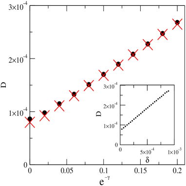
Figure 6: (color online). Theoretical (red $\times$ symbols) and numerical (black circles) values of the dispersion $D$ of an ensemble of $6\times 10^{4}$ finite-size particles about $1.8\times 10^{7}$ points representing $W^{u}(\Sigma)$. For the theoretical values, we use Eq. (7) (along with Eq. (9)). The values $\langle\lambda^{-1/2}\rangle=0.12$ and $\langle\lambda^{1/2}\rangle=21.06$ were computed numerically. The inset shows the dispersion $D$ of $6\times 10^{4}$ randomly generated points (at a distance $\delta\pi/2$ from the points of the chaotic saddle) about the same $1.8\times 10^{7}$ points representing $W^{u}(\Sigma)$. Interestingly, the overall scaling is linear in the range $3\times 10^{-5}<\delta<9\times 10^{-4}$. By regression, we obtain $F=7.128\times 10^{-5}+2.266\times 10^{-1}\times\delta$. The fact that $F(0)\neq 0$ is, of course, due to our approximation of $W^{u}(\Sigma)$ by a finite number of points.

VIII Conclusions

In summary, we have derived a theory accounting for the quantitative behaviour of the dispersion of neutrally buoyant finite-size particles about the unstable manifold of the chaotic saddle as a function of the Stokes parameter. Our theory refers to the onset of the finite-sizeness induced dispersion in the discrete description of the dynamics (second iterate of the map given by Eq. (5)). The theory involves a dynamical part, where the computation of the averages $\langle\lambda^{-1/2}\rangle$ and $\langle\lambda^{1/2}\rangle$ is required, and a geometrical part, regarding the function $F$. This geometrical part will be the same for any theory of the dispersion, either for higher iterates of the map, Eq. (5), or for snapshots in the continuous description, Eq. (2). It is a highly difficult problem to be solved analitically, but it can be overcomed by means of a computer-aided approach. The dynamical part of the theory will be different for higher iterates of the map or for snapshots in the continuous description, but it will be based on the same type of reasoning.

An interesting open problem is to determine the restrictions that the dispersion predicted by our theory imposes on the enhancement of activity (e.g. biological) toroczkai1 of finite-size particles.

- (1) H. Aref, J. Fluid Mech. 143, 1 (1984).
- (2) M. Horner, G. Metcalfe, S. Wiggins, and J.M. Ottino, J. Fluid Mech. 452, 199 (2002).
- (3) E.R. Abraham and M.M. Bowen, Chaos 12, 373 (2002).
- (4) T.-Y. Koh and B. Legras, Chaos 12, 382 (2002).
- (5) H. Kantz and P. Grassberger, Physica (Amsterdam) 17D, 75 (1985); G.-H. Hsu, E. Ott, and C. Grebogi, Phys. Lett. A 127, 199 (1988); T. Tél, in Directions in Chaos, edited by Hao Bai-Lin, (World Scientific, Singapore, 1990), Vol. 3, pp. 149-221.
- (6) G. Károlyi and T. Tél, Phys. Rep. 290, 125 (1997).
- (7) Finite-size effects are important not only for chaotic advection, but also in the turbulent regime. See, for instance, E. Balkovsky, G. Falkovich, and A. Fouxon, Phys. Rev. Lett. 86, 2790 (2001); J. Bec, Phys. Fluids 15, L81 (2003); R. Reigada, F. Sagués, and J. M. Sancho, Phys. Rev. E 64, 026307 (2001).
- (8) A. Babiano, J.H.E. Cartwright, O. Piro, and A. Provenzale, Phys. Rev. Lett. 84, 5764 (2000).
- (9) For the case of open chaotic advection of bubbles, see I.J. Benczik, Z. Toroczkai, and T. Tél, Phys. Rev. Lett. 89, 164501 (2002); I.J. Benczik, Z. Toroczkai, and T. Tél, Phys. Rev. E 67, 036303 (2003).
- (10) Z. Toroczkai, G. Károlyi, Á. Pentek, T. Tél, and C. Grebogi, Phys. Rev. Lett. 80, 500 (1998); G. Károlyi, Á. Pentek, Z. Toroczkai, T. Tél, and C. Grebogi, Phys. Rev. E 59, 5468 (1999); T. Tél, T. Nishikawa, A.E. Motter, C. Grebogi, and Z. Toroczkai, Chaos 14, 72 (2004).
- (11) There are situations where finite-sizeness leads to fractality. In this context, reactions were studied in the following papers: T. Nishikawa, Z. Toroczkai, and C. Grebogi, Phys. Rev. Lett. 87, 038301 (2001); T. Nishikawa, Z. Toroczkai, C. Grebogi, and T. Tél, Phys. Rev. E 65, 026216 (2002).
- (12) M.R. Maxey and J. Riley, Phys. Fluids 26, 883 (1983).
- (13) H. Aref, S.W. Jones, S. Mofina, and I. Zawadzki, Physica (Amsterdam) 37D, 423 (1989).
- (14) J.H.E. Cartwright, M.O. Magnasco, and O. Piro, Phys. Rev. E 65, 045203(R) (2002).
- (15) J.H.E. Cartwright, M.O. Magnasco, and O. Piro, Chaos 12, 489 (2002); J.H.E. Cartwright, M.O. Magnasco, O. Piro, and I. Tuval, Phys. Rev. Lett. 89, 264501 (2002).
- (16) A.E. Motter, Y.-C. Lai, and C. Grebogi, Phys. Rev. E 68, 056307 (2003).
- (17) J. Jacobs, E. Ott, and C. Grebogi, Physica (Amsterdam) 108D, 1 (1997).