Unsteady undular bores in fully nonlinear shallow-water theory

Abstract

We consider unsteady undular bores for a pair of coupled equations of Boussinesq-type which contain the familiar fully nonlinear dissipationless shallow-water dynamics and the leading-order fully nonlinear dispersive terms. This system contains one horizontal space dimension and time and can be systematically derived from the full Euler equations for irrotational flows with a free surface using a standard long-wave asymptotic expansion. In this context the system was first derived by Su and Gardner. It coincides with the one-dimensional flat-bottom reduction of the Green-Naghdi system and, additionally, has recently found a number of fluid dynamics applications other than the present context of shallow-water gravity waves. We then use the Whitham modulation theory for a one-phase periodic travelling wave to obtain an asymptotic analytical description of an undular bore in the Su-Gardner system for a full range of “depth” ratios across the bore. The positions of the leading and trailing edges of the undular bore and the amplitude of the leading solitary wave of the bore are found as functions of this “depth ratio”. The formation of a partial undular bore with a rapidly-varying finite-amplitude trailing wave front is predicted for “depth ratios” across the bore exceeding $1.43$. The analytical results from the modulation theory are shown to be in excellent agreement with full numerical solutions for the development of an undular bore in the Su-Gardner system.

I  INTRODUCTION

In shallow water, the transition between two different basic states, each characterized by a constant depth and horizontal velocity, is usually referred to as a bore. For sufficiently large transitions, the front of the bore is often turbulent, but as noted in the classical work of Benjamin and Lighthill [1], transitions of moderate amplitude are accompanied by wave trains without any wave breaking, and are hence called undular bores. Well-known examples are the bores on the River Severn in England and the River Dordogne in France. Undular bores also arise in other fluid flow contexts; for instance they can occur as internal undular bores in the density-stratified waters of the coastal ocean (see, for instance, [2], [3]), and as striking wave-forms with associated cloud formation in the atmospheric boundary layer (see, for instance, [4], [5]). They can also arise in many other physical contexts, and in plasma physics for instance, are usually called collisionless shocks.

The classical theory of shallow-water undular bores was initiated by Benjamin and Lighthill in [1]. It is based on the analysis of stationary solutions of the Korteweg - de Vries (KdV) equation modified by a small viscous term [6]. Subsequent approaches to the same problem have been usually based on the Whitham modulation theory (see [7], [8]), appropriately modified by dissipation; this allows one to study analytically the development of an undular bore to a steady state (see [9], [10], [11]). Most recently, this approach was used in [12] to study the development of an undular bore within the context of a bi-directional shallow-water model, based on an integrable version of the well-known Boussinesq equations, but modified by a small dissipative term.

However, a different class of problems arises when one neglects dissipation and considers only the dispersion-dominated transition between two basic states. Such a transition has the nonlinear oscillatory structure similar to classical undular bores but due to the absence of any dissipation, it remains unsteady and expands in time; consequently its qualitative properties and quantitative description are essentially different. This “conservative” undular bore evolution can be viewed as the initial stage of the eventual development of a steady weakly dissipative undular bore (see, for instance, the numerical simulations of unsteady undular bores in a set of Boussinesq equations describing weakly nonlinear long water waves in [13], and the analogous simulations for the full Euler equations with a free surface in [14], [15], [16]). Importantly, it also represents a universal mechanism for the generation of the solitary waves, which can be realized in several different fluid flow contexts. For instance, it occurs in the generation of solitary waves in trans-critical flow over topography (see [17], [18]), and in the formation of internal solitary waves in the coastal ocean [3] and atmosphere [5]. If the amplitude of the initial difference between the two basic states (e.g. a step in the simplest case) is small enough, the dynamics of an undular bore can be described by an integrable equation (typically the KdV equation). In this case one can take advantage of the exact methods of integration available for such equations. An asymptotic analytical description of an unsteady undular bore was first constructed in the framework of the KdV equation by Gurevich and Pitaevskii [19] using the Whitham modulation theory [7], [8]. The undular bore can then be described by a similarity solution of the Whitham modulation equations, obtained by an asymptotic singular reduction from the integrable KdV equation. Significantly in this integrable case, the modulation equations can be obtained in the Riemann invariant form. Later, this Gurevich-Pitaevskii theory has been generalised to other integrable equations such as the defocusing nonlinear Schrödinger equation [20], [21], [22], the Benjamin-Ono equation [23] and the Kaup-Boussinesq system [24]. All these cited works make essential use of the Riemann form of the modulation system, a feature associated with the complete integrability of the original equation.

In recent decades, largely due to extensive theoretical, numerical and experimental work on the internal solitary waves (see for instance [25], [26], [27], [28], [29] and references therein) it has become clear that although completely integrable systems may successfully capture many features of the propagation of weakly nonlinear waves, they may fail to provide an accurate description of finite-amplitude dispersive waves. Consequently, significant efforts have been directed towards the derivation of relatively simple models enabling the quantitative description of the propagation of fully nonlinear waves, and also amenable to analytical study. In the context of one-dimensional shallow-water waves such a model was derived using a long-wave asymptotic expansion of the full Euler equations for irrotational flow by Su and Gardner (SG) [30]. This system has the same structure as the well-known Boussinesq system for long water waves, but importantly for our purposes, retains full nonlinearity in the dispersive terms. For convenience, we will present a summary of this derivation in an Appendix. Later, it transpired that the SG equations coincide with the one-dimensional flat bottom reduction of another model derived by Green and Naghdi (GN) [31] for two-dimensional shallow-water waves. The GN model was obtained using the “directed fluid sheets” theory, which does not formally require an asymptotic decomposition, but instead imposes the condition that the vertical velocity has only a linear dependence on the vertical ($z$) coordinate, and simultaneously assumes that the horizontal velocity is independent of $z$. As a result, the incompressibility condition, the boundary conditions at the free surface and at the bottom and an energy equation are satisfied exactly. However, as pointed out in [32], this two-dimensional GN model has varying vorticity, even if initially the flow is irrotational. Thus, in the context of shallow-water waves propagating on an undisturbed uniform flow, this implication of the two-dimensional GN model contradicts the exact zero-vorticity requirement of solutions of the full Euler equations for flows which are initially irrotational. Thus, the physical validity of the original two-dimensional GN model for fully nonlinear shallow-water flows is suspect. This defect in the original GN system was recently removed in [33] where the principle of virtual work was combined with Hamilton’s principle expressed in Lagrangian coordinates to derive a new GN system (denoted as IGN) valid for irrotational flows. Nevertheless, the one-dimensional reduction of the original GN system, being equivalent to the SG system, and also to the one-dimensional reduction of the IGN system, does not have this disadvantage. But, although the SG and GN systems are mathematically equivalent in one spatial dimension, their physical meaning is essentially different as the two models are obtained, in fact, by quite different approximation methods.

We also note that the same SG (or GN) system of equations (but for different quantities) has appeared in the modelling of nonlinear wave propagation in continua with “memory” [34], bubbly fluids [35] and in solar magnetohydrodynamics [36]. With some modifications it has also been used for modelling short surface waves governed by the Euler equations [40] and for capillary-gravity waves [41]. The “two-layer” generalisation of the same one-dimensional fully nonlinear shallow-water system for large amplitude internal wave propagation has been obtained in [37] using asymptotic expansions and recently re-derived in [38] using Whitham’s Lagrangian approach [39]. Remarkably, despite the different physical origins of the governing equations, the consistent long-wave asymptotic procedure applied to this variety of fluid flows yields the same (quite peculiar) form of the nonlinear dispersive terms in the resulting system of equations. This is a clear indication of the universal nature of the dispersive term in the SG system of equations.

Thus, these equations (provided they are used in a consistent asymptotic approximation) represent an important mathematical model for understanding general properties of large-amplitude dispersive long waves. This is also supported by numerical evidence of the good agreement (superior to that for other generalized Boussinesq-type models) for vertically averaged features of numerical solutions of the full Euler equations in two dimensions (i.e. one vertical and one horizontal coordinate) describing flow over topography with numerical solutions of the GN (i.e. the SG) system (see [42]).

Note that, although in some of the mathematical literature it is customary to call even the one-dimensional version of the fully nonlinear shallow-water equations the Green-Naghdi system, here, to avoid confusion with the original, direct Green-Naghdi physical model, we will not use this term for the asymptotic system studied in this paper. Instead, we will call it the SG system, which would appear to be at least historically more correct.

While the properties of the permanent steady wave solutions of fully nonlinear systems have been intensively studied using analytical means, the properties of unsteady fully nonlinear dispersive waves and, in particular, the dynamics of dissipationless undular bores, remains largely unexplored from an analytical point of view. This absence of “unsteady” analytical results, analogous to those which can be obtained in weakly nonlinear wave theories, is due to the lack of an integrable structure for most fully nonlinear dispersive systems, thus preventing the use of the powerful methods of the inverse scattering theory. In this situation, an alternative approach is available through the afore-mentioned Whitham modulation theory, which allows one to obtain evolution equations for the local parameters of periodic travelling wave solutions. However, unlike the situation for the modulation equations associated with completely integrable equations, the modulation equations associated with non-integrable wave equations do not possess the Riemann invariant structure. This feature is a serious obstacle to their investigation.

However, recently an analytic approach has been developed in this case [43], [44], [45], which allows for the determination of a set of “transition conditions” across an unsteady undular bore, and which does not require the presence of the Riemann invariant structure for the Whitham modulation equations. This approach takes advantage of some specific properties of the Whitham modulation equations connected with their origin as certain averages of exact conservation laws, and so allows for exact reductions in the zero-amplitude and zero-wavenumber limits. As a result, the speeds of the boundaries of the undular bore region can be calculated in terms of the “depth ratio” across the undular bore, and also one then gets the amplitude of the lead solitary wave, a major parameter in observational and experimental data. This approach assumes the asymptotic validity of the modulation description of the undular bore, an assumption which can be inferred from the rigorous results available for completely integrable systems (see [46] and references therein). It is important, therefore, to compare the analytical results of the modulation approach with the results of direct numerical simulations in order to establish its validity in non-integrable problems.

In this paper, we use the afore-mentioned Whitham modulation theory to describe analytically unsteady undular bores in the fully nonlinear shallow water theory. This we will do for the whole range of allowed basic states. Then we will make a comparison with the full numerical solution of the original system for the same problem. Such a study, while elucidating some key properties of fully nonlinear shallow-water undular bores, is also a necessary step for understanding the more complicated dynamics of fully nonlinear internal undular bores, described by the “multi-layer” generalisation of the system under study in [37].

II.  GOVERNING EQUATIONS AND PERIODIC TRAVELLING WAVE SOLUTION
We consider the SG system describing fully nonlinear, unsteady, shallow water waves in the form [30]

$$\eta_{t}+(\eta u)_{x}=0\,,$$ (1)

$$u_{t}+uu_{x}+\eta_{x}=\frac{1}{\eta}\left[\frac{1}{3}\eta^{3}(u_{xt}+uu_{xx}-(u_{x})^{2})\right]_{x}\,.$$

Here $\eta$ is the total depth and $u$ is the layer-mean horizontal velocity; all variables are non-dimensionalised by their typical values. The first equation is the exact equation for conservation of mass and the second equation can be regarded as an approximation to the equation for conservation of horizontal momentum. The system (1) has the typical structure of the well-known Boussinesq-type systems for shallow water waves, but differs from them in retaining full nonlinearity in the leading-order dispersive term. Indeed, linearization of the right-hand side of the second equation about the rest state $\eta=1,u=0$ reduces the system (1) to a familar Boussinesq system (see, for instance, [47]). In Appendix A we show how the system (1) can be consistently obtained from the full irrotational Euler equations using an asymptotic expansion in the small dispersion parameter $\epsilon=h_{0}/L\ll 1$, where $h_{0}$ is the (dimensional) equilibrium depth and $L$ is a typical wavelength. We stress, however, that there is no limitation on the amplitude. Also we note that the system (1) represents a one-layer reduction of the system of Choi $\&$ Camassa [37] for fully nonlinear internal shallow-water waves and also has other physical applications already mentioned in the Introduction. The latter can be viewed as an indication that the nonlinear dispersive term in the right-hand side of the second equation in (1) has, to a certain degree, a universal nature. This suggests that the system (1) is an important mathematical model for understanding general properties of fully nonlinear fluid flows beyond the present shallow-water application. In particular, although in the context of shallow-water waves the system (1), as for any layer-mean model, is unable to reproduce the effects of wave overturning and becomes nonphysical for amplitudes greater than some critical value, it is instructive to study its solutions for the full range of amplitudes.

The linear dispersion relation of the SG system (1) relative to a constant basic state $\eta_{0},u_{0}$, has the form, for a right-propagating wave,

$$\omega_{0}(k)=k\left(u_{0}+\frac{\eta_{0}^{1/2}}{(1+\eta_{0}^{2}k^{2}/3)^{1/2}}\right)\,.$$ (2)

Here $\omega_{0}$ is the frequency of the linear waves and $k$ is the wavenumber.

The weakly nonlinear version of the SG system (1) is obtained by using the standard scaling $u=\mathcal{O}(\delta)$, $\eta=\eta_{0}+\mathcal{O}(\delta)$, $x=\mathcal{O}(\delta^{-1/2})$, $t=\mathcal{O}(\delta^{-3/2})$, where $\delta=\max[\eta-\eta_{0}]\sim\max u<<1$ is an amplitude parameter. For uni-directional propagation, this leads to the KdV equation for $\zeta=\eta-\eta_{0}$,

$$\partial_{t}\zeta+\partial_{x}\zeta+\frac{3}{2}\zeta\partial_{x}\zeta+\frac{1}{6}\partial^{3}_{xxx}\zeta=0\,$$ (3)

(see [37], [48]).

The first three conservation laws for the system (1) (there exists at least one more – see [37]) are obtained by simple algebraic manipulations and represent mass conservation, irrotationality and horizontal momentum conservation respectively,

$$\eta_{t}+(\eta u)_{x}=0\,,$$ (4)

$$\left(u+\frac{1}{6}\eta^{2}u_{xx}\right)_{t}+\left(\frac{u^{2}}{2}+\eta-\frac{\eta^{2}}{2}\left(u_{xt}+\frac{2}{3}uu_{xx}-(u_{x})^{2}\right)\right)_{x}=0\,,$$ (5)

$$(\eta u)_{t}+\left(\frac{\eta^{2}}{2}+\eta u^{2}-\frac{1}{3}\eta^{3}\left(u_{xt}+uu_{xx}-(u_{x})^{2}\right)\right)_{x}=0\,.$$ (6)

The periodic travelling wave solution of the SG system (1) is obtained from the ansatz $\eta=\eta(\theta)$, $u=u(\theta)$, where $\theta=x-ct$ and $c$ is the phase velocity. Substitution into the original system (1) and subsequent integration leads to

$$u=c-\frac{D}{\eta}\,,\ \ \ (\eta^{\prime})^{2}=\frac{3}{D^{2}}(-\eta^{3}+2B\eta^{2}-2C\eta+D^{2})\equiv\frac{3}{D^{2}}P(\eta)\,,$$ (7)

where $B,C,D$ are constants of integration. Introducing the roots of the polynomial

$$P(\eta)=-(\eta-\eta_{1})(\eta-\eta_{2})(\eta-\eta_{3})\,,\qquad\eta_{3}\geq\eta_{2}\geq\eta_{1}>0\,,$$ (8)

we get $D^{2}=\eta_{1}\eta_{2}\eta_{3}$. Equation (7) for the total depth $\eta$ can be solved in terms of the Jacobian elliptic function $\hbox{cn}(y;m)$:

$$\eta(\theta)=\eta_{2}+a\ \hbox{cn}^{2}\left(\frac{1}{2}\sqrt{\frac{3(\eta_{3}-\eta_{1})}{\eta_{1}\eta_{2}\eta_{3}}}\theta;m\right)\,,$$ (9)

$$\hbox{where}\qquad a=\eta_{3}-\eta_{2}\,,\qquad m=\frac{\eta_{3}-\eta_{2}}{\eta_{3}-\eta_{1}}$$ (10)

are the wave amplitude and the modulus respectively. The wavenumber is readily found from (7), (8) as

$$k=\frac{\pi\sqrt{3}}{\sqrt{\eta_{1}\eta_{2}\eta_{3}}}\left(\int\limits_{\eta_{2}}^{\eta_{3}}\frac{d\eta}{\sqrt{P(\eta)}}\right)^{-1}=\sqrt{\frac{3(\eta_{3}-\eta_{1})}{\eta_{1}\eta_{2}\eta_{3}}}\frac{\pi}{2K(m)}\,,$$ (11)

where $K(m)$ is the complete elliptic integral of the first kind. When $m=1$ ($\eta_{2}=\eta_{1}$) the cnoidal wave (9) becomes a solitary wave,

$$\eta=\eta_{s}(\theta)=(\eta_{3}-\eta_{1})\hbox{cosh}^{-2}\left(\frac{\sqrt{3(\eta_{3}-\eta_{1})}}{\sqrt{\eta_{3}}\eta_{1}}\theta\right)+\eta_{1}\,,$$ (12)

Next, we define averaging over the periodic family (7) by

$$\bar{F}(\eta_{1},\eta_{2},\eta_{3},c)=\frac{k}{2\pi}\int\limits^{2\pi/k}_{0}F(\theta;\eta_{1},\eta_{2},\eta_{3},c)d\theta=\frac{\sqrt{\eta_{3}-\eta_{1}}}{2K(m)}\int\limits^{\eta_{3}}_{\eta_{2}}\frac{F(\eta)}{\sqrt{P(\eta)}}d\eta\,,$$ (13)

where $F(\eta)\equiv F(\theta(\eta);\eta_{1},\eta_{2},\eta_{3},c)$. In particular,

$$\bar{\eta}=\frac{2}{\sqrt{\eta_{3}-\eta_{1}}}(\eta_{1}K(m)+(\eta_{3}-\eta_{1})E(m))\,,$$ (14)

$$\bar{u}=c-\frac{2\sqrt{\eta_{1}\eta_{2}}}{\sqrt{\eta_{3}(\eta_{3}-\eta_{1})}}\Pi_{1}\left(-\frac{\eta_{3}-\eta_{2}}{\eta_{3}},m\right);$$ (15)

$$\overline{\eta u}=\bar{\eta}c-\sqrt{\eta_{1}\eta_{2}\eta_{3}}\,.$$ (16)

Here $E(m)$ and $\Pi_{1}(\phi;m)$ are the complete elliptic integrals of the second and third kinds respectively.

Thus, the periodic solution of the SG equations (1) is characterised by four integrals of motion $\eta_{1},\eta_{2},\eta_{3},c$ or, equivalently, $\bar{\eta}$, $\bar{u}$, $k$, $a$. Next, if we allow them to be slowly-varying functions of $x$, $t$ and still require that the travelling wave (9) is a solution of the system (1) (to leading order in the small parameter characterizing the ratio of the spatial period of the travelling wave (9) to the typical scale for its variations in space) we arrive at the system of Whitham modulation equations.

III.  WHITHAM MODULATION EQUATIONS

There are several methods to obtain the modulation equations. We will follow here the original Whitham method of averaging the conservation laws [7], which is equivalent to formal multiple-scale asymptotic expansion [49], but is more convenient for our purposes.

To this end, we apply the averaging (13) to the conservation laws (4) – (6) considered for the periodic family (9). Due to the characteristic scale separation for the periodic solution and the modulations, the operations of differentiation and averaging asymptotically commute, and so we arrive at a set of quasilinear equations which can be represented in the form

$$\frac{\partial}{\partial t}\overline{P}_{j}(\bar{\eta},\bar{u},k,a)+\frac{\partial}{\partial x}\overline{Q}_{j}(\bar{\eta},\bar{u},k,a)=0\,,\quad j=1,2,3\,.$$ (17)

The system (17) should be closed by the wavenumber conservation law, which serves as a consistency condition in the formal asymptotic procedure equivalent to the Whitham averaging method (indeed, this equation can be obtained by averaging an extra conservation law and combining it with the averaged equations (17) [7], [8]),

$$\frac{\partial}{\partial t}k+\frac{\partial}{\partial x}\omega(\bar{\eta},\bar{u},k,a)=0\,.$$ (18)

The frequency $\omega$ in (18) is defined as

$$\omega=kc(\bar{\eta},\bar{u},k,a)\,,$$ (19)

where the phase speed $c$ is expressed in terms of the basic modulation variables with the aid of Eqs. (10), (11), (14), (15). We recall that typical $x,t$-scale for variations of the dependent variables in (17), (18) is much larger than that for the periodic travelling wave (9) itself in the original equations (1).

Using (4) – (6), (11), (13), we can readily obtain explicit expressions for the densities $\overline{P}_{j}$, $k$ and fluxes $\overline{Q}_{j}$, $\omega$ of the Whitham modulation system, in terms of the original parameters $\eta_{j}$, $c$ which are more convenient to use as intermediate modulation variables. These expressions involve complete elliptic integrals similar to the KdV case (see [8] for instance) but are, as expected, more cumbersome. The dependence of $\overline{P}_{j}$, $\overline{Q}_{j}$ on $\bar{\eta},\bar{u},k,a$ in (17) is then specified parametrically through Eqs. (10), (11), (14), (15).

Since we will use only some asymptotic properties of the Whitham system in the small amplitude and small wavenumber limits, we do not need to present the full expressions here. It is sufficient here to note that the modulation system of equations can be re-written in a generic quasi-linear form,

$${\bf y}_{t}+\mathrm{B}({\bf y}){\bf y}_{x}=0\,,$$ (20)

where ${\bf y}=(\bar{\eta},\bar{u},k,a)^{T}$ and the entries of the coefficient matrix are defined by $B_{ij}({\bf y})=\partial_{y_{i}}\overline{Q}_{j}/\partial_{y_{i}}\overline{P}_{j}$, $i,j=1,\dots,4$, and we define $P_{4}=k$, $Q_{4}=\omega$ . In some special cases, the Whitham systems can be represented in diagonal Riemann form, despite the fact that the number of the dependent variables exceeds two. This remarkable fact was first established by Whitham [7] for the third-order KdV modulation system, and then generalised to many other completely integrable systems (see [50] for a simple method of obtaining the Whitham system in Riemann form for a large class of integrable dispersive equations belonging to Ablowitz-Kaup-Newell-Segur (AKNS) hierarchy). The presence of the Riemann invariants dramatically simplifies further analysis of the modulation equations, and makes readily available many important particular solutions (see [21], [22], [24] for instance). However, for non-integrable equations such a structure is typically not available, which makes the corresponding analysis of the modulation system far more complicated.

There is no indication that the system (1) is integrable so the Whitham system (17), (18) is not likely to possess Riemann invariants. One can, in principle, calculate the characteristic velocities $\lambda_{j}\,,j=1,\dots 4$ for this system specified by the roots of the determinant $\det(\mathrm{B}-\lambda\mathrm{I})=0$ (where $\mathrm{I}$ is the unit matrix) but in the absence of the underlying algebraic structure, these expressions are unlikely to be amenable to analytic treatment. Instead, we can take advantage of some general properties of Whitham systems for obtaining the main quantitative features of the solutions, available even in the absence of integrability properties.

We now outline the properties of the Whitham system (17), (18) that distinguish it from the general class of hyperbolic quasilinear systems of fourth order. Most importantly, the Whitham system admits exact reductions for the linear $a=0$ and solitary wave $k=0$ regimes. It is clear that, since in both limits the oscillations do no contribute to the averaging (13), one has $\eta=\bar{\eta}$, $\bar{u}=u$, $\overline{\eta u}=\bar{\eta}\bar{u}$, and three averaged conservation laws (17) must reduce to the dispersionless shallow water equations for $\bar{\eta}$ and $\bar{u}$,

$$\bar{\eta}_{t}+(\bar{\eta}\bar{u})_{x}=0\,,\qquad\bar{u}_{t}+\bar{u}\bar{u}_{x}+\bar{\eta}_{x}=0\,.$$ (21)

At the same time, in each of the indicated limits, two out of the four characteristic families of the Whitham system must merge into a double characteristic to provide a consistent reduction to a hyperbolic system of a lower (third) order. Thus the limits $a\to 0$ and $k\to 0$ are singular ones for the modulation system. The detailed description of this reduction for a general class of nonlinear weakly dispersive systems can be found in [45]. Of course, for a specific system all the described properties can be established by a direct asymptotic analysis of the system (17), (18).

In the linear limit ($m\to 0$), for $c>0$ we get from Eqs. (10), (11), (14), (15) the modulation dispersion relation for linear waves propagating on the slowly varying background $\bar{\eta}(x,t)$, $\bar{u}(x,t)$,

$$a=0:\qquad\omega=\omega_{0}(\bar{\eta},\bar{u},k)=k\left(\bar{u}+\frac{\bar{\eta}^{1/2}}{(1+\bar{\eta}^{2}k^{2}/3)^{1/2}}\right)\,.$$ (22)

As expected, this is just the linear dispersion relation (2) for the right-propagating linear wave, where $u_{0}\mapsto\bar{u}$, $\eta_{0}\mapsto\bar{\eta}$.

In the solitary wave limit ($m\to 1$), we have from (14), (15) the speed-amplitude relation for a solitary wave propagating about the mean background $\bar{\eta}$, $\bar{u}$:

$$k=0:\qquad c=c_{s}(\bar{\eta},\bar{u},a)=\bar{u}+\sqrt{\bar{\eta}+a}\,.$$ (23)

We note that for the constant background flow formula (23) appears in Rayleigh [51]. It can be shown quite generally (see [45]) that the linear group velocity $\partial\omega_{0}/\partial k$, and the solitary wave speed $c_{s}$ coincide with the multiple characteristic velocities of the full modulation system (17), (18) in the limits $a\to 0$ and $k\to 0$ respectively, again, as expected.

One should emphasise here, that in contrast to the traditional analysis of linear and solitary wave propagation, the background flow parameters $\bar{\eta}$, $\bar{u}$ in this modulation theory are not constant in general, but vary slowly in $x,t$ over a typical modulation scale ($\Delta x\sim\Delta t\gg 1$) according to Eqs. (21). This $x,t$-dependence can be easily (parametrically) taken into account in the local initial-value problem analysis of the linear wave packet or solitary wave train propagation, which makes it essentially equivalent to the constant background flow case. However, in the undular bore problem, where the solitary waves and the linear wavepacket are restrained by being the parts of a global nonlinear wave structure, this dependence plays a crucial role.

We now present a weakly nonlinear asymptotic reduction of the modulation equations (17), (18), which will be important for our further analysis. One should emphasise that the small-amplitude expansion of the modulation system for equations (1) will not lead directly to the much-studied KdV modulation dynamics as the KdV asymptotics (3), along with small amplitudes, implies also a further long-wave scaling. We expand (17), (18) for $m\ll 1$ and express the result, using the representation of Eqs. (13)–(16) in terms of physical variables, rather than polynomial roots $\eta_{j}$. After a simple but somewhat lengthy calculation we obtain for $a\ll 1$ (see [8] for a similar representation for the KdV modulation system and [52] for nonlinear plasma wave modulation equations),

$$\frac{\partial\bar{\eta}}{\partial t}+\frac{\partial}{\partial x}(\bar{\eta}\bar{u}+A^{2})=0\,,$$ (24)

$$\frac{\partial}{\partial t}\bar{u}+\frac{\partial}{\partial x}\left(\frac{\bar{u}^{2}}{2}+\bar{\eta}+\mu(\bar{\eta},k)A^{2}\right)=\mathcal{O}(A^{2}\partial_{x}\bar{\eta},A^{2}\partial_{x}k,A^{2}\partial_{x}A^{2})\,,$$ (25)

$$\frac{\partial A^{2}}{\partial t}+\frac{\partial}{\partial x}\left(\frac{\partial\omega_{0}(\bar{\eta},\bar{u},k)}{\partial k}A^{2}\right)=\mathcal{O}(A^{2}\partial_{x}\bar{\eta},A^{2}\partial_{x}A^{2})\,,$$ (26)

$$\frac{\partial k}{\partial t}+\frac{\partial}{\partial x}\left(\omega_{0}(\bar{\eta},\bar{u},k)+\omega_{2}(\bar{\eta},k)A^{2}\right)=\mathcal{O}(A^{2}\partial_{x}\bar{\eta},A^{2}\partial_{x}k,A^{2}\partial_{x}A^{2})\,.$$ (27)

Here $\omega_{0}(\bar{\eta},\bar{u},k)$ is obtained from $\omega_{0}(k)$ given by Eq. (2) with $\eta_{0}$ and $u_{0}$ replaced with $\bar{\eta}$ and $\bar{u}$ as in (22). The values $A^{2}$, $\mu$, $\omega_{2}$ are expressed in terms of $\eta$, $k$, $a$ by the formulas

$$A^{2}=\overline{\eta u}-\bar{\eta}\bar{u}=\frac{a^{2}}{8\bar{\eta}^{1/2}(1+\kappa^{2})^{1/2}}+\mathcal{O}(a^{4})\,,\quad a\ll 1\,,$$ (28)

$$\mu=\frac{1+2\kappa^{2}-\kappa^{4}}{2\bar{\eta}^{1/2}(1+\kappa^{2})^{3/2}}\,,\qquad\omega_{2}=\frac{k}{\bar{\eta}}\frac{7\kappa^{4}+2\kappa^{2}+3}{8\kappa^{2}(1+\kappa^{2})};\qquad\kappa=k^{2}\bar{\eta}^{2}/3\,.$$ (29)

The wave energy equation (26) is obtained by subtracting the modulation equations (24) and (25), multiplied by $\bar{u}$ and $\bar{\eta}$ respectively, from the averaged momentum conservation equation $(\overline{\eta u})_{t}+(\dots)_{x}=0$. It is essential that the terms $\mathcal{O}(A^{2}\partial_{x}k)$ do not appear in the right-hand part of equation (26), i.e. the coefficient for $\partial_{x}k$ in the considered approximation is exactly $A^{2}\partial^{2}\omega_{0}(\bar{\eta},\bar{u},k)/\partial k^{2}$.

One can see that the system (24) – (27) indeed admits an exact reduction for $A=0$ (which is to say $a=0$) to the ideal shallow-water equations (21) for $\bar{\eta}$, $\bar{u}$ complemented by the wave conservation equation in the zero-amplitude limit:

$$A=0:\qquad\frac{\partial k}{\partial t}+\frac{\partial\omega_{0}(\bar{\eta},\bar{u},k)}{\partial x}=0\,,$$ (30)

An analogous asymptotic analysis can be performed for the solitary wave limit, when $(1-m)\ll 1$ (i.e. $k\ll 1$) resulting, for the limiting case $k=0$, in the same shallow-water reduction (21) complemented, instead of (30), by the equation for the solitary wave amplitude, which can be represented in the general form [52]

$$k=0:\qquad\frac{\partial a}{\partial t}+c_{s}(\bar{u},\bar{\eta},a)\frac{\partial a}{\partial x}+f_{1}(\bar{\eta},a)\frac{\partial\bar{u}}{\partial x}+f_{2}(\bar{\eta},a)\frac{\partial\bar{\eta}}{\partial x}=0\,.$$ (31)

where $f_{1,2}(\bar{\eta},a)$ are certain functions which can be, in principle, obtained by passage to the singular limit $k\to 0$ in the modulation system (17), (18). The actual calculation of this limit is significantly more cumbersome than in the linear case as one has to make the approximations up to exponentially small terms $\sim\exp(-1/k)$. We shall not derive the amplitude equation (31) here explicitly; instead, we will later take advantage of an alternative (conjugate) system of modulation variables enabling one to perform a singular zero-wavenumber limiting transition directly in the wavenumber conservation law (18).

IV.  UNSTEADY UNDULAR BORE TRANSITION

A. General construction

We shall consider initial conditions for the system (1) in the form of a step for the variables $\eta$ and $u$:

$$t=0:\ \ \ \eta=\eta^{-},\ \ u=u^{-}\ \hbox{for}\ x<0;\quad\eta=\eta^{+},\ u=u^{+}\,\hbox{for}\ x>0\,,$$ (32)

where $\eta^{\pm}$ and $u^{\pm}$ are constants. Without loss of generality, we will later set $\eta_{+}=1$ and $u^{+}=0$ for convenience.

We shall model the large-time asymptotic structure of the undular bore with the aid of an expansion fan solution of the Whitham system (17), (18) for the local parameters of the travelling wave (7). This approach to the modulation dynamics was first proposed by Gurevich and Pitaevskii [19] for the KdV equation, and has proved to be very effective for description of weakly nonlinear unsteady undular bores (see for instance [17], [18], and [3]). The Gurevich-Pitaevskii formulation has been extended to other integrable models such as the defocusing nonlinear Schrödinger equation [20], [21], [22] , the Benjamin-Ono equation [23] and the Kaup-Boussinesq system [24], [53]. The original Gurevich-Pitaevskii formulation makes essential use of the availability of the Riemann invariants for the modulation system. Its generalisation to the case when the Riemann invariants are not available has been recently developed in [43], [44], [45] and it is this approach that will be used in the present work.

We shall first assume that the modulation equations are hyperbolic and genuinely nonlinear for the solutions of interest, which implies that:
a) the characteristic velocities of the modulation system (17), (18) , $\lambda_{1}\geq\lambda_{2}\geq\lambda_{3}\geq\lambda_{4}$ are real and distinct for the solution of interest everywhere except those special lines in the $x,t$-plane where two of them collapse into a double eigenvalue of the Whitham system;
a) the characteristic fields $dx/dt=\lambda_{j}(\bar{\eta},\bar{u},k,a)$ are not linearly degenerate, i.e.
${\bf r}_{j}\cdot\hbox{grad}\lambda_{j}\neq 0$, where ${\bf r}_{j}(\bar{\eta},\bar{u},k,a)$ is the right eigenvector of the coefficient matrix $\mathrm{B}$ in (20) corresponding to the eigenvalue $\lambda_{j}$ [54].

The first condition ensures the modulational stability of the solution under study. Two properties of the SG system (1) relevant to this issue can be readily inferred from its general structure:
i) the linearised eigenmode problem for the system (1) yields pure real eigenvalues (the frequencies in the linear dispersion relation (2) are real for all values of $k$); ii) the dispersionless limit of full equations (1) is a strictly hyperbolic shallow-water system.
Also we note the recent result in [55] where the stability of solitary waves with respect to linear perturbations has been established using the Evans function technique for a one-dimensional Green-Naghdi system mathematically equivalent to (1). All this, however, does not guarantee the modulational stability of nonlinear travelling waves (9) with $0<m<1$. This can be established by the analysis of the characteristic velocities of the nonlinear modulation system (17) for the class of solutions of interest. The general condition for hyperbolicity of the modulation system for the one-dimensional Green-Naghdi equations in Lagrangian variables has been derived in [34], but the actual verification of this condition represents an involved technical task, possibly not resolvable by analytical means. Later we will establish and explicitly verify a more particular criterion of the modulational stability of the undular bores in the system (1) using the asymptotic system (24) – (27). As to the genuine nonlinearity issue, we will show below that the modulation system for Eqs. (1) admits linear degeneration of one of the characteristic fields for a certain domain of the initial conditions (32), and will derive an important restriction connected with the formation of partial undular bores in Section 5.

According to the general Gurevich-Pitaevskii scheme [19], we replace the original initial-value problem (32) for the system (1) with a matching problem for the mean flow at the free boundaries (i.e. the edges of the undular bore). Specifically, we require the continuity of $\bar{\eta},\bar{u}$ along the lines $x=x^{-}(t)$, $x=x^{+}(t)$ defined by the conditions of zero amplitude (trailing edge) and zero wavenumber (leading edge) respectively, i.e.

$$\begin{array}[]{l}x=x^{-}(t):\qquad a=0\,,\ \ \bar{\eta}=\eta^{-}\,,\ \ \bar{u}=u^{-}\,,\\ x=x^{+}(t):\qquad k=0\,,\ \ \bar{\eta}=\eta^{+}\,,\ \ \bar{u}=u^{+}\,.\end{array}$$ (33)

The edges of the undular bore at $x=x^{\pm}(t)$ represent free boundaries, and their determination is a part of the solution to be obtained. Since for the step-like initial data (32) the problem reformulation in terms of the averages does not contain any parameters of the length dimension the solution of the quasi-linear Whitham equations (20) must depend on the similarity variable $s=x/t$ alone. The boundaries $x^{\pm}(t)$ then represent straight lines $x=s^{\pm}t$, where $s^{\pm}$ are the speeds of the undular bore edges which should be found in terms of the given initial step parameters.

The similarity solution of the Whitham equations can be represented in the general form

$$F_{i}(\bar{\eta},\bar{u},k,a)=I_{i}\,,\qquad\lambda_{j}(\bar{\eta},\bar{u},k,a)=s\,,\qquad i=1,2,3\,,$$ (34)

where $I_{i}$ are constants and $\lambda_{j}$ is one of the characteristic velocities of the modulation system (17), (18). They must be chosen so that the solution satisfies the matching conditions (33). As a result, the solution (34) yields a slow $x,t$-dependence of the parameters $\bar{\eta},\bar{u},k,a$ of the periodic solution (9) so that after substitution of (34) into (9) we arrive at a slowly modulated nonlinear wave degenerating into a linear wavepacket near the trailing edge, and gradually transforming into a chain of successive solitary waves close to the leading edge (see figure 1). This wave structure corresponds to the observable features of unsteady undular bores (see, for instance, [56] and [3] for laboratory and natural observations and [13], [14], [15], [16] for numerical simulations), and has been rigorously recovered as the small-dispersion asymptotics of the exact solution of certain integrable equations (see the review [46] and references therein).

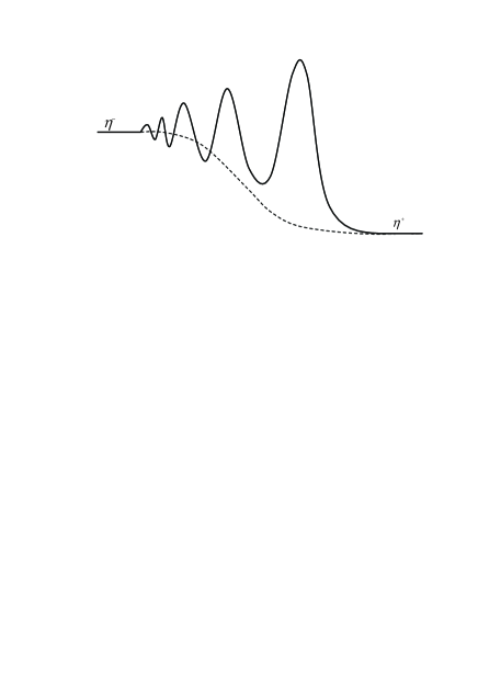
Figure 1: Oscillatory structure of the undular bore evolving from an initial step (dashed line).

Explicit modulation solutions in the form of an expansion fan (34) have been constructed for a number of integrable (by the inverse scattering transform) bi-directional equations where the functions $F_{i}$ represent Riemann invariants of the modulation system (see for instance [24] and references therein). We emphasise, however, that the general similarity solution (34) can, in principle, be constructed for any quasi-linear hyperbolic system and, as such, is available for the Whitham system (20) regardless of the existence of the Riemann invariants. Therefore, the Gurevich-Pitaevskii construction in fact does not rely on the integrability of the system in the sense of the availability of an inverse scattering transform.

The fact that the modulation system admits exact reductions as $a\to 0$ and $k\to 0$ to the dispersionless limit equations (21), complemented by the wave number conservation law in the corresponding limit (see Section 3) allows one to study the limiting structure of the integrals $F_{i}$ in the expansion fan solution (34) without necessarily constructing the solution itself. Remarkably, these limiting integrals can be expressed in terms of the linear dispersion relation of the original system, and one of its “dispersionless” nonlinear characteristic velocities. The corresponding analysis has been recently described in [43], [44], [45] for a rather broad class of equations that one may characterize as $2\times 2$ strictly hyperbolic modified by weak dispersion. As a result, a set of the transition conditions has been obtained, which allow one to fit the undular bore into the classical solution of the shallow water equations much as the classical shock is fitted into the ideal gas dynamics solution without constructing the detailed solution in the transition region. Next we derive explicit expressions for these conditions for the undular bore in the SG system (1). Our analytical results are compared with numerical simulations of the full system (1). An outline of the numerical method is given in the Appendix B.

B.  Simple undular bore transition relation

Since the number of the constants in the solution (34) is three, whereas the initial conditions (32) are characterised by four constants, there should be an additional relationship

$$\Phi(\eta^{+},\eta^{-},u^{+},u^{-})=0\,,$$ (35)

for the admissible values of the variables at the edges of the undular bore. This relationship has been shown in [44], [45] to follow from the continuous matching of the characteristics of the Whitham system (17), (18) and the ideal shallow water system (21) for the “external” flow at the undular bore boundaries. Such a reformulation of the problem in terms of characteristics is equivalent to the original matching conditions (33) and yields the relationship (35) in the form of the zero-jump condition across the undular bore for one of the classical Riemann invariants. For the right-propagating shallow-water undular bore it assumes the form

$$\frac{u^{-}}{2}-\sqrt{\eta^{-}}=\frac{u^{+}}{2}-\sqrt{\eta^{+}}\,.$$ (36)

Generally, the step initial condition (32) resolves into a combination of two waves: an undular bore(s) and/or a rarefaction wave(s). The family of the initial steps which resolve into a single right-propagating undular bore described by the expansion fan solution of the Whitham equations is distinguished by the condition (36), which coincides with the relationship between $u$ and $\eta$ for the simple wave of compression in the limit of the dispersionless equations (see [8] for instance). We shall call the undular bores satisfying condition (36), simple undular bores. Of course, for a left-propagating simple undular bore, the transition relation is obtained from the zero jump condition for another analogous classical shallow-water Riemann invariant.

Without loss of generality one can put in (36) $u^{+}=0\,,\eta^{+}=1$ so that the simple undular bore transition curve becomes

$$u^{-}=2(\sqrt{\eta^{-}}-1)\,$$ (37)

and yields all the admissible states upstream of the undular bore provided the flow downstream is fixed as above.

Figure 2: Riemann invariant (dashed line) and the shock-wave (dotted line) transition curves

We emphasise that this simple undular bore transition condition does not coincide with the classical jump relation obtained from a combined consideration of the balance of mass and momentum across the bore provided its width is constant (which is the case both for turbulent bores and for established frictional undular bores - see for instance [8];[12]):

$$u^{-}=(\eta^{-}-1)\sqrt{\frac{1+\eta^{-}}{2\eta^{-}}}\,.$$ (38)

The curves (37) and (38) are shown in figure 2 and demonstrate high contact for small jumps, which is expected in view of the well-known fact that the Riemann invariant has only a third order jump across a weak shock. Thus, the distinction between the jump condition (38) and the simple undular bore transition relation (37) becomes noticeable only for large-amplitude undular bores. This distinction may not seem very important from a practical point of view as the shallow-water undular bores are known to exist only for $\eta^{-}/\eta^{+}\lessapprox 1.3$ (see [1], [8], [14]) after which they become turbulent with wave breaking. However, it is the simple undular bore curve (37) (rather than the jump condition (38)) that is consistent with the modulation system, and allows analytic determination of the undular bore location. Also, equations (1) appear in other physical systems as well as in the shallow water context (see [34], [35], [36]), where different physical restrictions may apply and a wider range of amplitudes may be involved.

C. Undular bore location and lead solitary wave amplitude
Let this similarity solution of the Whitham equations be confined to the interval $s^{-}t\leq x\leq s^{+}t$ so that the modulation provides a transition of the underlying travelling wave (9) from a linear wavepacket ($a=0$) at the trailing edge to a solitary wave ($k=0$) at the leading edge. Then the speeds of the undular bore edges $s^{\pm}$ can be determined by the general expressions derived in [43], [44], [45]. Below we briefly outline how this method applies to the SG system (1).

The analysis in [43], [44], [45] is based on the general fact that, due to the degeneration of the three averaged “hydrodynamic” conservation laws (17) for $a=0$ and $k=0$ into the second-order dispersionless system (the shallow-water system (21) for $\bar{\eta}$ and $\bar{u}$ in our case) the boundaries of the undular bore necessarily correspond to multiple characteristics of the Whitham modulation equations. The corresponding multiple characteristic speeds can then be obtained without a full integration of the Whitham system by deriving the solution in the form (34). To this end, one complements the matching conditions (33) by the definition of the edges using natural kinematic conditions at the free boundaries $x=s^{\pm}t$. Namely, at the trailing edge we require that the edge speed to coincide with the linear group velocity, and at the leading edge it coincides with the leading solitary wave speed, that is

$$s^{-}=\frac{\partial\omega_{0}}{\partial k}(\eta^{-},u^{-},k^{-})\,,\qquad s^{+}=c_{s}(\eta^{+},u^{+},a^{+})\,,$$ (39)

where $\omega_{0}(\bar{\eta},\bar{u},k)$, $c_{s}(\bar{\eta},\bar{u},a)$ are given by (22), (23). These kinematic conditions (39) contain unknown parameters $k^{-}$ and $a^{+}$, which need to be found in terms of the given initial jumps for $\eta$ and $u$.

The described degeneration of the Whitham modulation equations in the limits $a=0$ and $k=0$ implies the existence of two families of integrals: $\{a=0,\Phi_{1}(\bar{u},\bar{\eta})=C_{1}$, $\Phi_{2}(k,\bar{\eta})=C_{2}\}$ and $\{k=0,\Phi_{1}^{*}(\bar{u},\bar{\eta})=C_{1}^{*}$, $\Phi_{2}^{*}(a,\bar{\eta})=C_{2}^{*}\}$ where $C_{1,2}$, $C_{1,2}^{*}$ are constants. In the context of the similarity solutions these integrals represent the zero-amplitude and zero-wavenumber “sections” of the general integrals $F_{j}$ in the full solution (34). However, the “limiting” integrals $\Phi_{1,2}$, $\Phi^{*}_{1,2}$ can be found directly from the reductions of the Whitham equations as $a=0$ and $k=0$. The constants $C_{1,2}$, $C_{1,2}^{*}$ are then found from the matching conditions (33) and the transition curve (36). As a result, we find that the parameters $k^{-}$ and $a^{+}$ are obtained from the functions $k(\bar{\eta})$ and $a(\bar{\eta})$ at $\bar{\eta}=\eta^{-}$ and $\bar{\eta}=\eta^{+}$ respectively.

Indeed, for $a=0$ the Whitham system (17), (18) reduces to a third-order system consisting of the shallow-water equations for the mean flow (21) complemented by the wave conservation equation (30) for linear waves. Then, substituting $\bar{u}=\bar{u}(\bar{\eta})$ and $k=k(\bar{\eta})$ into (21), (30) we obtain the integrals

$$\bar{u}\pm 2\sqrt{\bar{\eta}}=C_{1}\,,\qquad\frac{dk}{d\bar{\eta}}=\frac{\partial\omega_{0}(\bar{\eta},\bar{u}(\bar{\eta}),k)/\partial\bar{\eta}}{\bar{u}(\bar{\eta})\mp\sqrt{\bar{\eta}}-\partial\omega_{0}/\partial k}\,.$$ (40)

It is shown in [45] that the ordinary differential equation in (40) is just the equation for the characteristic integral of the full modulation system along the multiple characteristic on which $a=0$ and thus, its integral specifies, from the first equation in Eq. (39), the speed of the trailing edge of the undular bore. The signs and constants of integration in (40) are then found from the transition relation (36) and the matching conditions (33).

The reduction of the Whitham system for $k=0$ consists of the shallow-water system (21) and the amplitude equation (31). Analogously to the zero-amplitude case, one can obtain the integrals $\bar{u}(\bar{\eta})$, $a(\bar{\eta})$ and then, from the second equation in Eq. (39), the leading edge speed of the undular bore. There is, however, the afore-mentioned technical complication connected with obtaining the amplitude modulation equation (31) from Eqs. (17), (18) in the limit $k\to 0$. This difficulty is bypassed in the papers of [43], [44], [45] by the introduction of the conjugate wavenumber

$$\tilde{k}=\frac{\pi\sqrt{3}}{\sqrt{\eta_{1}\eta_{2}\eta_{3}}}\left(\int\limits_{\eta_{1}}^{\eta_{2}}\frac{d\eta}{\sqrt{P(\eta)}}\right)^{-1}$$ (41)

instead of the amplitude $a$ in the modulation equations and considering the (singular) limiting transition as $k\to 0$ in the wavenumber conservation law (18). Then, the equation for the characteristic integral $\tilde{k}(\bar{\eta})$ turns out to coincide with the equation for its zero-amplitude counterpart $k(\bar{\eta})$ (40), but the linear dispersion relation $\omega_{0}(\bar{\eta},\bar{u},k)$ should be replaced with the conjugate expression $\tilde{\omega}_{s}=-i\omega_{0}(\bar{\eta},\bar{u},ik)$.

We now apply this construction to the description of the undular bore transition in fully nonlinear shallow-water system (1). Again, for simplicity, we put $\eta^{+}=1$, $u^{+}=0$ in the downstream flow. Then the expressions for the speeds of the edges of the undular bore take the form

$$s^{-}=\frac{\partial\Omega_{0}}{\partial k}(\eta^{-},k^{-})\,,\qquad s^{+}=\frac{\Omega_{s}(1,\tilde{k}^{+})}{\tilde{k}^{+}}\,.$$ (42)

Here the functions $\Omega_{0}(\bar{\eta},k)$ and $\Omega_{s}(\bar{\eta},\tilde{k})$ can be expressed in terms of the linear dispersion relation for the modulations (22),

$$\Omega_{0}(\bar{\eta},k)=\omega_{0}(\bar{\eta},\bar{u}(\bar{\eta}),k)\,,\quad\Omega_{s}(\bar{\eta},\tilde{k})=-i\Omega_{0}(\bar{\eta},i\tilde{k})\,,$$ (43)

where $\bar{u}(\bar{\eta})=2(\sqrt{\bar{\eta}}-1)$, that is

$$\Omega_{0}(\bar{\eta},k)=2k(\bar{\eta}^{1/2}-1)+\frac{k\bar{\eta}^{1/2}}{(1+\bar{\eta}^{2}k^{2}/3)^{1/2}}\,.$$ (44)

The parameters $k^{-}$ and $\tilde{k}^{+}$ in (42) are calculated as the boundary values $k^{-}=k(\eta^{-})$, $\tilde{k}^{+}=\tilde{k}(1)$ of the functions $k(\bar{\eta})$ and $\tilde{k}(\bar{\eta})$, which in turn are defined by the ordinary differential equations

$$\frac{dk}{d\bar{\eta}}=\frac{\partial\Omega_{0}/\partial\bar{\eta}}{V(\bar{\eta})-\partial\Omega_{0}/\partial k}\,,\qquad k(1)=0\,,$$ (45)

$$\frac{d\tilde{k}}{d\bar{\eta}}=\frac{\partial\Omega_{s}/\partial\bar{\eta}}{V(\bar{\eta})-\partial\Omega_{s}/\partial\tilde{k}}\,,\qquad\tilde{k}(\eta^{-})=0\,,$$ (46)

where

$$V(\bar{\eta})=\bar{u}(\bar{\eta})+\bar{\eta}^{1/2}=3\bar{\eta}^{1/2}-2.$$ (47)

Substituting (44) into (45) and introducing $\alpha=(1+\bar{k}^{2}\bar{\eta}^{2}/3)^{-1/2}$ as a new variable instead of $k$ we obtain the ordinary differential equation,

$$\frac{d\bar{\eta}}{\bar{\eta}}=\frac{2(1+\alpha+\alpha^{2})}{\alpha(1+\alpha)(\alpha-4)}d\alpha\,,\quad\alpha(1)=1\,.$$ (48)

Since (48) has a separated form, we can integrate it to obtain

$$\bar{\eta}=\frac{1}{\sqrt{\alpha}}\left(\frac{4-\alpha}{3}\right)^{21/10}\left(\frac{1+\alpha}{2}\right)^{2/5}\,.$$ (49)

Next, using (42), (44) we get an implicit expression for the trailing edge $s^{-}$ in terms of the total depth ratio across the undular bore $\Delta=\eta^{-}/\eta^{+}=\eta^{-}$:

$$\sqrt{\beta}\Delta-\left(\frac{4-\beta}{3}\right)^{21/10}\left(\frac{1+\beta}{2}\right)^{2/5}=0\,,\quad\hbox{where}\ \ \beta=\left(\frac{2+s^{-}}{\sqrt{\Delta}}-2\right)^{1/3}\,.$$ (50)

Similarly, using the conjugate linear dispersion relation (43) and the equation (46) we obtain from (42), the equation of the leading edge $s^{+}=s^{+}(\Delta)$ in an implicit form,

$$\frac{\Delta}{\sqrt{s^{+}}}-\left(\frac{3}{4-s^{+}}\right)^{21/10}\left(\frac{2}{1+s^{+}}\right)^{2/5}=0\,.$$ (51)

We emphasise that Eqs. (50), (51) are exact solutions of the modulation equations for a fully nonlinear wave regime.

Figure 3: The leading $s^{+}$ (upper curve) and the trailing $s^{-}$ (lower curve) edge speeds vs the depth ratio $\Delta$ across the simple undular bore. Dashed line: modulation solution (50), (51); Diamonds: values of $s^{+}$, $s^{-}$ extracted from the full numerical solution; Dotted line: the KdV modulation solution (53).

The graphs of $s^{+}$, $s^{-}$ versus the depth ratio $\Delta$ across the bore are shown in figure 3 (dashed line) and demonstrate excellent agreement with the results of direct numerical simulations (solid line) of the system (1) for $\Delta<\Delta_{cr}\approx 1.43$ where $\Delta_{cr}$ corresponds to the minimum of the function $s^{-}(\Delta)$. We will discuss the reason for the discrepancy between the modulation predictions for the leading edge and numerical results for large depth ratios $\Delta>\Delta_{cr}$ in Section 6.

Next, we consider the correspondence between these exact expressions (51), (50) for a fully nonlinear undular bore, and the weakly nonlinear KdV asymptotics (53). Thus, we introduce in (50),(51) a small parameter $\delta=\Delta-1\ll 1$ to obtain the expansions

$$s^{+}=1+\delta-\frac{5}{12}\delta^{2}+\mathcal{O}(\delta^{3})\,,\qquad s^{-}=1-\frac{3}{2}\delta+\frac{23}{8}\delta^{2}+\mathcal{O}(\delta^{3})\,.$$ (52)

On the other hand, for the KdV equation we have from the original Gurevich-Pitaevskii (1973) solution, taking into account the coefficients in the KdV equation (3),

$$s_{KdV}^{+}=1+(\Delta-1)\,,\qquad s_{KdV}^{-}=1-\frac{3}{2}(\Delta-1)\,.$$ (53)

Thus, the expansions (52) agree to first order with the KdV formulas (53).

It can be seen from the numerical solution shown in figure 3 and from the asymptotic expansion (52) of the analytic solution (51) that, for large initial jumps the leading edge of the undular bore in the fully nonlinear model (1) demonstrates a tendency towards a slower speed compared with its weakly nonlinear counterpart. This feature agrees with the results of numerical simulations of undular bores in other fully nonlinear models of Boussinesq type and of the full Euler equations for potential flows [15], [16].

At the same time, one can see that the trailing edge of the undular bore in the fully nonlinear shallow-water dynamics described by the SG system (1) is noticeably shifted forward compared with that of the KdV solution. As a result, the fully nonlinear undular bore transition is significantly narrower than that predicted by the weakly nonlinear theory. This feature was noted in [16], where shallow-water undular bores were studied using a fully nonlinear numerical model without further long-wave expansions. This result that the SG system (1), while formally derived as a long-wave model, can adequately reproduce the features associated with the propagation of short waves (the dynamics of the trailing edge of the undular bore), is due to the fact that system (1) has a better approximation of the full linear dispersion relation than the KdV equation. Indeed, the linear dispersion relation (2) can be regarded as a Padé approximation of the exact expression $(\omega_{0}-ku_{0})^{2}=k\tanh k\eta_{0}$ following from the Euler equations, whereas the KdV dispersion relation is a less accurate Taylor series approximation. Applications of modifications of system (1) to the description of the nonlinear dynamics of short waves have been considered in [40], [41].

Figure 4: The lead solitary wave amplitude vs depth ratio $\Delta$. Solid line: numerical solution; dashed line: modulation solution (54)

From the expression (23) relating the speed and the amplitude of the SG solitary wave, and the definition of the leading edge (39) $s^{+}=c_{s}(\eta^{+},a^{+})$ we derive the equation for the amplitude of the leading solitary wave for the free surface elevation,

$$\frac{\Delta}{(a^{+}+1)^{1/4}}-\left(\frac{3}{4-\sqrt{a^{+}+1}}\right)^{21/10}\left(\frac{2}{1+\sqrt{a^{+}+1}}\right)^{2/5}=0\,.$$ (54)

The expansion of (54) for small jumps $\delta=\Delta-1$ yields $a^{+}=2\delta+\delta^{2}/6+\mathcal{O}(\delta^{3})$ which agrees to first order with the well-known KdV expression $a^{+}_{KdV}=2(\Delta-1)$ obtained by Gurevich and Pitaevskii [19]. The graph of $a^{+}$ versus the depth ratio $\Delta$ is shown in figure 4 (dashed line) and agrees with the results of direct numerical simulations (solid line). Again, the discrepancy for $\Delta>\Delta_{cr}\approx 1.43$ will be discussed in the next section.

One should bear in mind that formulae (50), (51), and (54) were obtained for simple undular bores i.e. they are valid only if the initial levels in $\eta$ and $u$ satisfy the Riemann invariant condition (37). For an arbitrary initial discontinuity the resolution will occur via a combination of two simple waves (undular bore(s) and/or rarefaction wave(s)) propagating in opposite directions in a certain reference frame. The relevant combination is found by determining the pair of intersecting transition (simple-wave) curves in the $\eta-u$ plane with their centres at the initial basic states, in a similar manner to the construction of decay diagrams in gas dynamics (where one of the waves could be a classical shock satisfying the Rankine-Hugoniot curve); see [57] for instance. An important example of such a two-wave resolution occurs in the dam-break problem and will be considered in Section VII.

The construction of the transition conditions for a simple undular bore, described above, is subject to the inequalities

$$u^{-}-\sqrt{\eta^{-}}<s^{-}<u^{-}+\sqrt{\eta^{-}}\,,\quad u^{+}+\sqrt{\eta^{+}}<s^{+}\,,\quad s^{+}>s^{-}\,.$$ (55)

These inequalities are analogous to the entropy conditions of classical gas dynamics (see for instance [54]) and ensure that only three of the four “dispersionless” characteristics families of the shallow water system (21): $x/t=u^{\pm}\pm\sqrt{\eta^{\pm}}$ transfer initial data (32) from the $x$-axis into the undular bore domain in the $(x,t)$-plane providing consistency with the number of parameters in the similarity solution (34) (see [45] for details). A direct verification shows that conditions (55) are satisfied for all values of $\Delta$.

Figure 5: The numerical solution of the system (1) for the initial depth ratio $\Delta=1.2$, $t=250$. Initial step data: $\eta^{-}=\Delta=1.2,\ u^{-}=2(\sqrt{\eta^{-}}-1)$, $\eta^{+}=1,\ u^{+}=0$

Next, we briefly describe the results of the direct numerical simulations used to obtain the graphs in figures 3,4. The numerical method itself is outlined in the Appendix B. A typical numerical solution for an undular bore is shown in figure 5, where we plot the surface elevation $\eta$. The initial profiles for $\eta$ and $u$ are chosen so that the simple undular bore condition (37) is satisfied for the asymptotic states at infinity. As a result, a backward propagating rarefaction wave does not form, and the resolution of the step occurs through the undular bore alone. In contrast with the model pattern shown in figure 1 the numerically obtained solution contains small-amplitude oscillations behind the undular bore. These are essentially linear oscillations arising due to the deviation of the initial perturbation used in the numerical simulations from the Heaviside step function. Indeed, these oscillations decrease in amplitude proportionally to $t^{-1/2}$, as expected in a linear theory. A detailed analysis of these linear oscillations behind the undular bore region can be found in [58], where collisionless shocks in a two-temperature plasma were studied. The trailing edge position of the undular bore in the numerical solution is found by using a linear approximation of the amplitude profile, which will be shown in the next section to be consistent with the asymptotic modulation solution.

Although, as we will show in the next section, from an analytical point of view the linear dependence of the wave amplitude on position is valid only in the vicinity of the trailing edge of the undular bore, the linear numerical interpolation of the undular bore envelope turns out to be quite accurate for a significant part of the undular bore (for moderate values of the jumps across the bore) and can be used for the determination of the trailing edge position in the numerical solution despite the fact that the rear end of the undular bore is visually obscured by the above-mentioned linear oscillations (see figure 5).

The zero-amplitude point in figure 5 corresponds to a “degenerate contact discontinuity” which moves with the velocity $u_{c}=u^{-}<s^{-}$. This point (a characteristic in the $x-t$ plane) is an analog of the contact discontinuity of classical gas dynamics, although in our present dissipationless case there is no discontinuity forming here.

V.  MODULATION SOLUTION IN THE VICINITY OF THE TRAILING EDGE

Next, we study the asymptotic behaviour of the modulation solution in the vicinity of the (given) trailing edge $s=s^{-}(\Delta)$ defined by (50) provided that $\Delta<\Delta_{cr}$. Since the amplitude of the oscillations near the trailing edge of a fully developed undular bore is small, we can use the asymptotic modulation system (24)–(27). Assuming that the mean flow variations in the vicinity of the trailing edge of the undular bore are induced entirely by the wave motion we introduce the asymptotic decompositions

$$\bar{\eta}=\eta_{0}+A^{2}\eta_{2}(k)+\dots\,,\qquad\bar{u}=u_{0}+A^{2}u_{2}(k)+\dots\ \,,$$ (56)

where $\eta_{0}$, $u_{0}$ is a a constant flow, and substitute them into the asymptotic modulation equations (24), (25). We assume that (this will be confirmed by the actual solution)

$$A^{2}\partial_{x}A^{2}\ll A^{2}\partial_{x}k\ll\partial_{x}A^{2}\,.$$ (57)

Then consistently to leading order in $A$ we get

$$\eta_{2}=-\frac{(3-\kappa_{0}^{2})(1+\kappa_{0}^{2})^{5/2}}{2\sqrt{\eta_{0}}\kappa_{0}^{2}(\kappa_{0}^{4}+3\kappa_{0}^{2}+3)}\,,\qquad u_{2}=-\frac{2\kappa_{0}^{6}+5\kappa_{0}^{4}+8\kappa_{0}^{2}+3}{2\eta_{0}\kappa_{0}^{2}(\kappa_{0}^{4}+3\kappa_{0}^{2}+3)}\,,$$ (58)

where $\kappa_{0}^{2}=k^{2}\eta_{0}^{2}/3$. Then, substituting (56), (58) into the modulation equations (26), (27) we obtain the classical modulation equations for a weakly nonlinear wavepacket (see [8], Ch.14)

$$\frac{\partial A^{2}}{\partial t}+\omega^{\prime}_{0}(k)\frac{\partial A^{2}}{\partial x}+\omega_{0}^{\prime\prime}A^{2}\frac{\partial k}{\partial x}=\mathcal{O}(A^{2}\partial_{x}A^{2},A^{4}\partial_{x}k)\,,$$ (59)

$$\frac{\partial k}{\partial t}+\omega^{\prime}_{0}(k)\frac{\partial k}{\partial x}+\tilde{\omega}_{2}(k)\frac{\partial A^{2}}{\partial x}=\mathcal{O}(A^{2}\partial_{x}A^{2},A^{2}\partial_{x}k)\,,$$ (60)

where $\omega_{0}(k)\equiv\omega_{0}(\eta_{0},u_{0},k)$ is given by (2) and

$$\tilde{\omega}_{2}(k)=-\frac{k(3\kappa_{0}^{8}+\kappa_{0}^{6}+14\kappa_{0}^{4}+33\kappa_{0}^{2}+9)}{8\eta_{0}\kappa_{0}^{2}(1+\kappa_{0}^{2})(\kappa_{0}^{4}+3\kappa_{0}^{2}+3)}<0$$ (61)

is an effective weakly nonlinear correction to the frequency $\omega_{0}(k)$, including the effect of the induced mean flow.

The characteristic velocities of the system (59), (60) are readily found, and have the form

$$\lambda_{\pm}=\omega_{0}^{\prime}\pm\sqrt{\omega_{0}^{\prime\prime}\tilde{\omega}_{2}}A+\mathcal{O}(A^{2})\,.$$ (62)

Thus the modulation system is hyperbolic if $\omega_{0}^{\prime\prime}\tilde{\omega}_{2}>0$, which is the classical Lighthill criterion for modulational stability of a weakly nonlinear wavepacket (see [8], [59] for instance). Since here

$$\omega_{0}^{\prime\prime}=-\frac{k\eta_{0}^{5/2}}{(1+k^{2}\eta_{0}^{2}/3)^{5/2}}<0$$ (63)

we infer that the weakly nonlinear wave trains of the system (1) are modulationally stable for all $k$ provided condition (57) is satisfied.

Next we construct the similarity solution of the system (59), (60) satisfying the boundary condition

$$x=s^{-}t:\qquad A=0\,,\ \ k=k^{-}\,,$$ (64)

where $s^{-}(\Delta)$ is defined by (50) and $k^{-}(\Delta)$ is found from Eq. (49) evaluated at $\bar{\eta}=\Delta$. This similarity solution of equations (59), (60) subject to conditions (64), and an additional condition $dk/ds<0$ distinguishing the right-propagating undular bore, has the form

$$k=k^{-}+\frac{2}{3\omega_{0}^{\prime\prime}(k^{-})}(s-s^{-})+\mathcal{O}(s-s^{-})^{2}\,,$$ (65)

$$A=\frac{1}{3\sqrt{\omega_{0}^{\prime\prime}(k^{-})\tilde{\omega}_{2}(k^{-})}}(s-s^{-})+\mathcal{O}(s-s^{-})^{2}\,,$$ (66)

where $\omega_{0}^{\prime\prime}(k)$ and $\tilde{\omega}_{2}(k)$ are given by Eqs. (63), (61). The asymptotic solution for $\bar{\eta}$, $\bar{u}$ is given by (58). We see that the solution (66) in view of (28) implies a linear growth in amplitude $a\sim A\sim(x-x^{-})$ near the trailing edge of the undular bore for a given $t$. One can see now that conditions (57) used in the derivation of the weakly nonlinear reduction (59), (60) of the modulation system are indeed satisfied for the obtained solution (65), (66) so that the whole construction is consistent throughout.

VI.  FORMATION OF A FINITE-AMPLITUDE REAR WAVE FRONT
The existence of a minimum for the trailing edge speed $s^{-}$ as a function of the depth ratio $\Delta$ across the undular bore (see figure 3) suggests that there is a possibility of wave-front formation at the rear end of the undular bore when $\Delta=\Delta_{cr}$. Indeed, as $s^{-}$ from (39) has the interpretation as a linear group velocity, there is an analogy with the classical situation of the formation of the rapid wave front in linear wave theory (see [8] Ch. 11). In that case the existence of a real root $k=k^{*}$ for the equation $\omega_{0}^{\prime\prime}(k)=0$ implies that the group velocity has a minimum (or maximum) at $k=k^{*}$, so that the wave packet cannot propagate with a speed lower (greater) than $\omega_{0}^{\prime}(k^{*})$; consequently a wavefront forms beyond which the wave amplitude decays rapidly to zero. From the viewpoint of modulation theory, this implies a local linear degeneration of the wave number conservation law

$$\frac{\partial k}{\partial t}+\omega_{0}^{\prime}(k)\frac{\partial k}{\partial x}=0\,$$ (67)

in the vicinity of a critical point $k=k^{*}$. Of course, as is well known (see [8]) this rapid change occurs only in the asymptotic theory, the full solution for the wave front transition in linear theory is described by an Airy function, and is characterised by an exponential decay in the wave amplitude outside the front.

A nonlinear analog of this classical wave front formation has been recently noted in [60] for an undular bore solution of the Camassa-Holm (CH) equation, which is a certain weakly nonlinear uni-directional approximation of the SG equations (1) (see [48]). For the special family of periodic peakon-type solutions of the CH equation, considered in [60], the modulation system consists of just two equations, say for $k$ and $\omega$, and its expansion fan solution exhibits a turning point for the nonlinear characteristics of the modulation system, so that the wave cannot propagate back beyond some $x=x^{*}$. Behind this point the solution decays exponentially. The turning point for the nonlinear characteristics is a nonlinear analog of the minimum for the linear group velocity. Indeed, the linear dispersion relation for the CH equation allows for real roots for the equation $\omega_{0}^{\prime\prime}(k)=0$ corresponding to the the classical linear wave front formation.

In the present case of the system (1), the second derivative of the linear dispersion relation (2) never vanishes (see (63)). However, in the full modulation theory $\omega_{0}=\omega_{0}(\bar{\eta},\bar{u},k)$ (see Eq. (22)) and the condition for wave front formation should be formulated in general terms of the linear degeneration of the characteristic field, rather than just the simple vanishing of the second derivatives of the linear dispersion relation. The $j$-th characteristic field $\lambda_{j}$ of the quasilinear system of conservation laws is called linearly degenerate [54] if

$${\bf r}_{j}\cdot\hbox{grad}\lambda_{j}=0\,,$$ (68)

where ${\bf r}_{j}$ is the right eigenvector corresponding to the eigenvalue $\lambda_{j}$, i.e. the characteristic velocity has an extremum in the direction orthogonal to its “own” characteristic direction. For the Whitham system (17), (18) the eigenvalues and eigenvectors are defined in terms of an equivalent standard representation (20) by

$$\{\lambda_{j}:\ \det(\mathrm{B}-\lambda\mathrm{I})=0\}\,;\qquad\mathrm{B}\,\mathbf{r}_{j}=\lambda_{j}\mathbf{r}_{j}\,.$$ (69)

In the SG modulation system, the condition (68) means that the linear degeneration takes place at the point of the minimum for the characteristic velocity $\lambda_{k}$ in the expansion fan similarity solution (34). As the solution implies $d\lambda_{j}/ds>0$, the lower bound for the characteristic velocity range in the undular bore is determined by the trailing edge speed, hence the first appearance of the linear degeneration of the characteristic field $\lambda_{j}$ as $\Delta$ grows is expected at the trailing edge where the wave amplitude vanishes. Thus the occurrence of the linear degeneration point on the undular bore profile is indeed determined by the minimum of the curve $s^{-}(\Delta)$,

$$\frac{ds^{-}}{d\Delta}=0\,,$$ (70)

which yields $\Delta_{cr}\approx 1.43$ (see figure 3).

It is instructive to also obtain the value of $\Delta_{cr}$ directly from the definition (68). We consider the zero-amplitude reduction of the full modulation system with the built-in simple-wave relation $\bar{u}=2(\sqrt{\bar{\eta}}-1)$, which is an exact integral of the ideal shallow-water equations (21) and which is consistent with the relationship (37) between $u$ and $\eta$ at the trailing edge of the undular bore,

$$\frac{\partial\bar{\eta}}{\partial t}+V(\bar{\eta})\frac{\partial\bar{\eta}}{\partial x}=0\,,\qquad\frac{\partial k}{\partial t}+\frac{\partial\Omega_{0}(\bar{\eta},k)}{\partial x}=0\,,$$ (71)

where $V(\bar{\eta})$, $\Omega_{0}(\bar{\eta},k)$ are given by Eqs. (47), (44). Thus for the limiting case under study,

$$\mathrm{B}=\left(\begin{array}[]{cc}V(\bar{\eta})&0\\ \partial\Omega_{0}(\bar{\eta},k)/\partial\bar{\eta}&\partial\Omega_{0}(\bar{\eta},k)/\partial\bar{k}\\ \end{array}\right)\,,$$ (72)

and an elementary calculation yields

$$\lambda_{2}=\frac{\partial\Omega_{0}(\bar{\eta},k)}{\partial k}\,,\qquad{\bf r}_{2}=\left(1,\ \frac{\partial\Omega_{0}(\bar{\eta},k)/\partial\bar{\eta}}{V(\bar{\eta})-\partial\Omega_{0}(\bar{\eta},k)/\partial k}\right)^{T}$$ (73)

so that the orthogonality condition (68) takes the form,

$$\frac{\partial^{2}\Omega_{0}(\bar{\eta},k)}{\partial k\ \partial\bar{\eta}}+\frac{\partial^{2}\Omega_{0}(\bar{\eta},k)}{\partial k^{2}}\frac{\partial\Omega_{0}(\bar{\eta},k)/\partial\bar{\eta}}{V(\bar{\eta})-\partial\Omega_{0}(\bar{\eta},k)/\partial k}=0\,.$$ (74)

Note that (74) is a “two-dimensional” analog of the condition $\omega_{0}^{\prime\prime}(k)=0$ for the single wavenumber conservation law (67). After substitution of $\Omega_{0}(\bar{\eta},k)$ and $V(\bar{\eta})$ Eq. (74) becomes

$$4\alpha^{5}-8\alpha^{4}-11\alpha^{3}+2\alpha^{2}+2\alpha+2=0\,$$ (75)

where $\alpha=(1+k^{2}\bar{\eta}^{2}/3)^{-1/2}<1$. The only real root of (75), which is less than unity, is $\alpha_{0}\approx 0.661$. The intersection of the curve $\alpha(\bar{\eta},k)=\alpha_{0}$ with the integral (49) relating $k$ and $\bar{\eta}$ at the trailing edge of the undular bore yields the critical value of the density ratio across the simple undular bore and the corresponding wavenumber at its trailing edge (see figure 5):

$$\Delta_{cr}\approx 1.430\,,\qquad k^{-}\approx 1.376$$ (76)

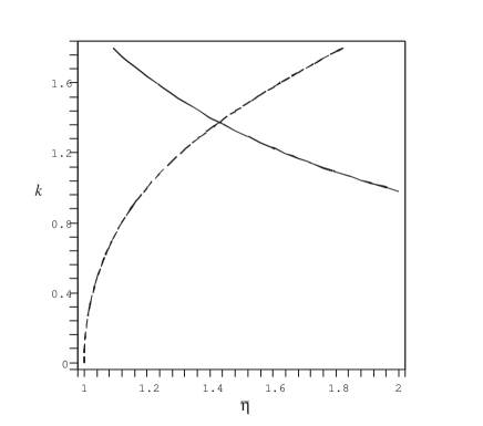
Figure 6: The intersection of the linear degeneration curve $\alpha(\bar{\eta},k)=\alpha_{0}$ (solid line) with the dependence $k(\bar{\eta})$ at the trailing edge given by (49) (dashed line) yields the critical value of $\Delta\approx 1.43$

Figure 7: The supercritical, partial undular bore for $\Delta=3.5$, $t=120$. Initial step data: $\eta^{-}=\Delta,\ u^{-}=2(\sqrt{\Delta}-1)$, $\eta^{+}=1,\ u^{+}=0$

The corresponding values of other parameters at this point are: $u^{-}\approx 0.392$, $s^{-}\approx 0.737$. It is readily shown from the ordinary differential equation (45) for $k(\bar{\eta})$ that the linear degeneration condition (74) considered for the trailing edge of the undular bore is equivalent to the condition (70).

The numerical solutions for different $\Delta$ show that, as $\Delta$ increases further beyond $\Delta_{cr}$, the point of linear degeneration shifts towards the leading edge of the undular bore so that a “partial undular bore” with a finite-amplitude rapidly-varying (on the modulation scale) rear wave front forms (see figure 7). To determine the speed of a rear finite-amplitude wave front in the partial undular bore of this type one should use the general expression (68) rather than its zero-amplitude version (74). An important consequence of the occurrence of the rear wave front is that the Gurevich-Pitaevskii type formulation used so far, is not applicable for $\Delta>\Delta_{cr}$ as it is based on the assumption of a fully developed undular bore with a zero-amplitude trailing edge, which in its turn implies the natural continuity matching conditions (33) for the mean height and velocity at the trailing edge. Instead, for $\Delta>\Delta_{cr}$ the conditions at the wave front should presumably be formulated in terms of the original Whitham shock conditions for the modulations [7], [8] following from the averaged conservation laws (17), (18).

Thus, we reach a different problem formulation for $\Delta>\Delta_{cr}$, and this explains some of the discrepancy in figure 3 between the numerical and modulation solutions for the leading edge $s^{+}(\Delta)$ (and correspondingly for the amplitude $a^{+}(\Delta)$ in figure 4) as the modulation solution constructed in Section V is based on the assumption of a fully developed undular bore with the natural boundary conditions (33) satisfied at its edges. Curiously, the numerical curve for the trailing edge in figure 3 constructed using the formal linear approximation for the undular bore envelope, $a\sim x-x^{-}$, still agrees very well with the formal modulation solution for the zero-amplitude trailing edge despite the fact that such a trailing edge itself is already nonexistent! Thus, the formal modulation solution (50), (51) can still be used to estimate the width of moderate-amplitude undular bores. Of course, one should bear in mind that this discussion does not essentially affect the shallow-water application of the system (1), as then undular bores exist only for $\Delta\lessapprox 1.3$ ([1], [8]), and for such undular bores the modulation theory is in exact correspondence with the full numerical solution.

Although the detailed description of the structure of supercritical, partial undular bores is beyond the scope of the present work, one can infer some qualitative features of such undular bores from an asymptotic analysis of the modulations in the vicinity of the trailing edge for the undular bore corresponding to $\Delta\approx\Delta_{cr}$, i.e. in the “nearly-critical” configuration. For $\Delta\approx\Delta_{cr}$ the rear wavefront is not yet pronounced and the wave amplitude close to it is still small as in the vicinity of usual trailing edge. The asymptotic behaviour of the modulations near such an emerging wave front, however, will differ from that for the trailing edge for “normal” undular bores described in Section V in that the linear degeneration of the characteristic field at the wave front will result in a square root variation of amplitude with position, $a\sim(x-x_{-})^{1/2}$, rather than the universal linear behaviour $a\sim(x-x_{-})$, as in (66). This can be understood by considering the characteristic velocities of the reduced modulation system (59) and (60) near the turning point where the system is close to a linear degeneration, i.e. when $\omega_{0}^{\prime\prime}(k)=\mathcal{O}(A^{2})\ll 1$. Indeed, in this situation the corresponding expansion of the eigenvalues $\lambda_{\pm}$ (see (62)) would have the form $\lambda_{\pm}=\omega_{0}^{\prime}(k)+\mathcal{O}(A^{2})$, which implies the square root behaviour of the self-similar solution for the amplitude $a\sim A\sim(s-s^{-})^{1/2}$. One can expect qualitatively the same behaviour for the full asymptotic modulation theory described by the system (24)–(27), for which the condition for linear degeneration is more complex (see (74)). This explains the visually noticeable change in the undular bore envelope shape from nearly linear to convex when $\Delta$ increases (cf. figures 5 and 7). While for $\Delta-\Delta_{cr}=\mathcal{O}(1)$ one should not expect the same square root asymptotic behaviour of the amplitude near the (finite-amplitude) wavefront, one can see from figure 7 that the supercritical undular bore retains the same convex envelope shape. We note that a qualitatively similar type of wave envelope behaviour occurs for undular bores for the CH equation, in which case the rear wavefront is always present [60].

As we have already mentioned, the continuous modulation solution does not describe the rapid exponential decay of the wave amplitude at the rear wavefront (see [60]). One can, however, retain the modulation description by introducing appropriate discontinuities in the modulation variables using the conservative form of the modulation equations (17) and (18). Such formal, discontinuous modulation solutions were proposed by Whitham in [7], but have not been employed so far.

The presence of jumps for modulations at the rear wave front implies that the Riemann invariant condition (37), which is a consequence of the continuous characteristic matching [44], [45] is no longer valid. As a result, for $\Delta>\Delta_{cr}$ this condition no longer prevents the generation of a backward rarefaction wave. This is clearly seen in figure 7 where numerical solution is presented for the decay of a large initial step with $\Delta=3.5$ with the values $\eta^{-}=\Delta$ and $u^{-}$ initially satisfying the Riemann invariant condition $u^{-}=2(\sqrt{\eta^{-}}-1)$. Surprisingly, as our analysis of numerical solutions shows, these “supercritical” undular bores apparently follow the classical shock curve (38), which is quite unexpected for dissipationless wave dynamics. Indeed, the classical shock curve occurs under these conditions where the transition zone of constant width forms either due to dissipation, or due to the existence of a steady smooth bore solution for the original equations (see, for instance, the internal bore solution in [37]). As our numerical solution shows, the supercritical undular bores for the SG system are unsteady, so the mechanism leading to the occurrence of the classical bore conditions is not clear. We plan to investigate this effect in a separate study.

In conclusion, one should mention that partial undular bores of the above described type are different from the partial undular bores occurring in initial-boundary value problems for nonlinear dispersive systems (see [61] for the description of such a partial undular bore in KdV theory). Indeed, the latter occur owing to the presence of the boundary conditions and retain the main qualitative properties of regular undular bores, while the former are characterised by the formation of a linearly degenerate wavefront (which is absent in the KdV theory) and have a qualitatively different envelope shape.

VII.  DAM-BREAK PROBLEM

We next consider the classical dam-break problem. Let a separator (a dam) hold back water of some depth, say $\Delta_{0}>1$ while the water in front of the dam has unit depth. The dam breaks at $t=0$ and releases the water downstream. Thus, we are dealing with the decay of the initial discontinuity:

$$t=0:\ \ \ \eta=\Delta_{0}>1,\ \ u=0\ \ \hbox{for}\ \ x<0;\quad\eta=1,\ \ u=0\,\ \hbox{for}\ x>0\,$$ (77)

for the equations (1). We first assume that $\Delta_{0}$ is not too large, so that the generated undular bore is “subcritical”, i.e. fully developed.

Figure 8: Numerical solution of the dam-break problem for $\eta$. Initial total depth jump $\Delta_{0}=1.8$, $t=150$

Figure 9: Numerical solution of the dam-break problem for $u$. Initial total depth jump $\Delta_{0}=1.8$, $t=150$

Since the discontinuity (77) does not satisfy the simple undular bore transition relation (37), two waves must occur after the dam breaking. Simple analysis shows that the relevant combination consists of a right-propagating simple undular bore, and a left-propagating centred rarefaction wave (see figures 8,9). Then the depth ratio across the undular bore is found from the intersection of the transition curve (37) and the centred left-propagating rarefaction wave curve $\sqrt{\Delta_{0}}={u^{-}}/{2}+\sqrt{\eta^{-}}$, where $\eta^{-}$, $u^{-}$ are the parameters of a constant mean flow in the region separating the undular bore and the rarefaction wave. As a result we get

$$\eta^{-}=\frac{(\sqrt{\Delta_{0}}+1)^{2}}{4}\,,\qquad u^{-}=2(\sqrt{\eta^{-}}-1)\,.$$ (78)

For instance, if $\Delta_{0}=1.8$ as in figures 8 and 9, then from (78) we have $\eta^{-}=1.37$, $u^{-}=0.34$, which agrees with the full numerical solution (of course, this illustration concerns the mathematical model itself, and is beyond its scope of applicability to actual shallow-water undular bores).

It is easily seen from Eq. (78) that $\eta^{-}<\Delta_{0}$. The critical value of $\Delta_{0}$ corresponding to $\eta^{-}=\Delta_{cr}=1.43$ is $1.94$ so that for $\Delta_{0}>1.94$ we get a partial undular bore satisfying the jump condition (38). To get the dependence of the lead solitary wave amplitude on the initial depth ratio one should set Eq. (78) into the equation (54). For small $\delta_{0}=\Delta_{0}-1$ we have the expansion

$$a^{+}=\delta_{0}-\frac{1}{12}\delta_{0}^{2}+\mathcal{O}(\delta_{0}^{3})\,,$$ (79)

To compare the small-amplitude expansion (79) with the corresponding weakly nonlinear, uni-directional KdV result one should use the “effective” initial jump $\delta=\eta^{-}-1$, where $\eta^{-}$ is calculated using Eq. (78), as the value of an initial discontinuity in the KdV equation. One can then see that the classical KdV result $a^{+}=2\delta$ agrees with the first term of the expansion (79).

The distinct oscillations generated at the right boundary of the rarefaction wave in the numerical plots in Figs. 8,9 are due to resolution of the weak discontinuity which would be present here in the rarefaction wave solution for the dispersionless shallow-water equations. These linear oscillations are universally described by the Airy function and have been studied in [58]. Unlike the linear oscillations just behind the undular bore, which decay with time as $t^{-1/2}$ the amplitude of the oscillations generated near the right boundary of the rarefaction wave decay as $t^{-1/3}$.

VIII  CONCLUSIONS

We have studied the undular bore transition connecting two different constant basic states in the fully nonlinear shallow-water model described by the SG equations (1) derived using shallow-water approximation in the full Euler system for irrotational flows. The main feature of the undular bore transition is its unsteady character, due to the absence of dissipation in the model. Such an expanding undular bore can be represented as a slowly modulated periodic wave with the modulations governed by the Whitham modulation equations. The wave is confined to an expanding interval $s^{-}t<x<s^{+}t$, where $s^{+}$ and $s^{-}$ are the speeds of the leading and the trailing edge respectively. The modulation is such that close to the leading edge the wave assumes the form of successive solitary waves while close to the trailing edge it degenerates into small-amplitude harmonic wave.

Using some special properties of the Whitham equations in the small-amplitude (linear) and small-wavenumber (solitary wave) limits we have obtained exact analytic expressions for the speeds $s^{\pm}$ and the lead solitary wave amplitude $a^{+}$ as functions of the depth ratio $\Delta$ across the undular bore. These results differ from those derived previously for the weakly nonlinear case described by the KdV equation. In particular, the fully nonlinear theory predicts a substantially narrower undular bore transition even for moderate values of the depth ratios across the bore. It is also shown that one should use the zero-jump condition for the ideal shallow-water Riemann invariant across the bore, rather than classical jump conditions applicable to an established steady-state undular bores with small dissipation. Our analysis is performed for the whole range of $\Delta$. It is shown that a critical value exists $\Delta_{cr}\approx 1.43$ corresponding to the minimum of the relation $s^{-}(\Delta)$, so that in undular bores with $\Delta>\Delta_{cr}$ a rapidly-varying finite-amplitude rear wave front forms instead of a zero-amplitude trailing edge, characteristic for small-amplitude undular bores. Such an effect is absent in weakly nonlinear KdV theory, but has recently been observed in the more sophisticated Camassa-Holm model.

Parallel to the modulational analysis, we have carried out some direct numerical simulations of undular bore development in the fully nonlinear shallow-water model (1). Excellent agreement of the modulation solution with the parameters drawn from the full numerical solution has been demonstrated for “subcritical” ($\Delta<\Delta_{cr}$) undular bores. The occurrence of a rear finite-amplitude wave front for $\Delta>\Delta_{cr}$ predicted by the modulation analysis is also confirmed. Such an agreement can be regarded as a striking confirmation of validity of the Whitham modulation theory in unsteady fully nonlinear wave problems, where the exact methods of integrable soliton theory are often not applicable.

Acknowledgements

The authors thank E. Ferapontov and V. Khodorovskii for useful discussions.

Appendix A: Derivation of the SG system

For convenience, we here produce a brief summary of the derivation of the system (1) originally derived in [30]. The equations of motion for fully nonlinear irrotational water waves are, when expressed in long-wave coordinates $X=\epsilon x,T=\epsilon t,z$,

$$\epsilon^{2}\phi_{xx}+\phi_{zz}=0\,,$$

$$w=0\quad\hbox{at}\quad z=0\,,$$

$$\eta_{T}+\phi_{X}\eta_{X}=\frac{1}{\epsilon}w\,\quad\hbox{at}\quad\,z=\eta\,,$$

$$\phi_{T}+\frac{1}{2}\{u^{2}+w^{2}\}+\eta=0\quad\hbox{at}\quad z=\eta\,.$$

Here the horizontal and vertical velocity are given by

$$u=\phi_{X}\,,\quad w=\frac{1}{\epsilon}\phi_{z}\,.$$

First we have the exact equation for conservation of mass, which is the first equation in (1),

$$\eta_{T}+(U\eta)_{X}=0\,,$$

$$\hbox{where}\quad\eta\,U=\int_{0}^{\eta}\,u\,dz\,.$$

Next we expand $\phi$ in powers of $\epsilon^{2}$,

$$\phi=F(X,T)-\epsilon^{2}\frac{z^{2}}{2}F_{XX}+\cdots\,,$$

$$\hbox{so that}\quad u=F_{X}-\epsilon^{2}\frac{z^{2}}{2}F_{XXX}+\cdots\,,$$

$$\hbox{and}\quad w=-\epsilon zF_{XX}+\cdots\,,$$

$$\hbox{Also}\quad U=F_{X}-\epsilon^{2}\frac{\eta^{2}}{6}F_{XXX}+\cdots\,.$$

Systematic replacement of $F_{X}$ with the mean flow $U$ yields

$$F_{X}=U+\epsilon^{2}\frac{\eta^{2}}{6}U_{XX}+\cdots\,,$$

$$u(z=\eta)=U-\epsilon^{2}\frac{\eta^{2}}{3}U_{XX}+\cdots\,,$$

$$w(z=\eta)=\epsilon\eta U_{X}+\cdots\,.$$

Hence the Bernoulli condition at the the free surface becomes

$$F_{T}-\epsilon^{2}\frac{\eta^{2}}{2}U_{XT}+\frac{1}{2}\{U^{2}-\epsilon^{2}\frac{2\eta^{2}}{3}UU_{XX}+\epsilon^{2}\eta^{2}U_{X}^{2}\}+\eta=0\,.$$

Finally, differentiation with respect to $X$ yields

$$U_{T}+UU_{X}+\eta_{X}=\epsilon^{2}\frac{1}{3\eta}\{\eta^{3}(U_{XT}+UU_{XX}-U_{X}^{2})\}\,,$$

This is the second equation in (1). Note that only terms of $O(\epsilon^{2})$ are needed, and that $w$ is linear in $z$ to this order.

Appendix B: Numerical Method

During the development of modulation theory for the fully nonlinear shallow-water equations, comparisons have been made between predictions of this theory for various properties of an undular bore and the results of full numerical solutions of the equations under study. Here, a brief outline will be given of the numerical method used to solve the system (1).

The first of the equations (1) was solved using the Lax-Wendroff method (see [62] for instance). To solve the second equation, the time and space derivatives were approximated using standard second order, centred finite differences. This resulted in a stable numerical scheme that was second order in both the time $\Delta t$ and space $\Delta x$ steps. Due to the $(\eta^{3}u_{xt})_{x}$ term in the second equation (1), solving for $u$ required the solution of a tri-diagonal system of equations for $u$ at the new time step. In the numerical solutions shown in the present work, $\Delta x$ varied from $10^{-2}$ to $10^{-3}$ and $\Delta t$ varied from $10^{-3}$ to $10^{-4}$.

Figure Captions

• Figure 1.
  Oscillatory structure of the undular bore evolving from an initial step (dashed line).

• Figure2.
  Riemann invariant (dashed line) and the shock-wave (dotted line) transition curves.

• Figure 3.
  The leading $s^{+}$ (upper curve) and the trailing $s^{-}$ (lower curve) edge speeds vs the depth ratio $\Delta$ across the simple undular bore. Dashed line: modulation solution (50), (51); Diamonds: values of $s^{+}$, $s^{-}$ extracted from the full numerical solution; Dotted line: the KdV modulation solution (53).

• Figure 4.
  The lead solitary wave amplitude vs depth ratio $\Delta$. Solid line: numerical solution; dashed line: modulation solution (54).

• Figure 5.
  The numerical solution of the system (1) for the initial depth ratio $\Delta=1.2$, $t=250$. Initial step data: $\eta^{-}=\Delta=1.2,\ u^{-}=2(\sqrt{\eta^{-}}-1)$, $\eta^{+}=1,\ u^{+}=0$.

References

- [1] T.B. Benjamin and M.J. Lighthill, “On cnoidal waves and bores,” Proc. Roy. Soc. A224, 448 (1954).
- [2] R. Grimshaw, “Internal solitary waves,” in Environmental Stratified Flows, ed. by R. Grimshaw, (Kluwer, Boston, 2002) p.1.
- [3] J.P. Apel, “ A new analytical model for internal solitons in the ocean” Journ. Phys. Oceanogr. 33, 2247 (2003).
- [4] J.W. Rottman and R. Grimshaw, 2001 “Atmospheric internal solitary waves,” in Environmental Stratified Flows, ed. by R. Grimshaw (Kluwer, Boston, 2002) p. 61.
- [5] A. Porter and N.F. Smyth, “Modelling the morning glory of the Gulf of Carpentaria,” J. Fluid Mech. 454, 1 (2002).
- [6] R.S. Johnson, “A non-linear equation incorporating damping and dispersion,” J. Fluid Mech. 42, 49 (1970).
- [7] G.B. Whitham, “Non-linear dispersive waves,” Proc. Roy. Soc. London, 283A, 238 (1965).
- [8] G.B. Whitham, Linear and Nonlinear Waves, (Wiley, New York, 1974).
- [9] A.V. Gurevich and L.P. Pitaevskii, “Averaged description of waves in the Korteweg-de Vries-Burgers equation,” Sov. Phys. JETP 66, 490 (1987).
- [10] V.V. Avilov, I.M. Krichever, and S.P. Novikov, “Evolution of Whitham zone in the theory of Korteweg-de Vries,” Sov. Phys. Dokl., 32, 564 (1987).
- [11] S. Myint and R.H.J. Grimshaw, “The modulation of nonlinear periodic wavetrains by dissipative terms in the Korteweg-de Vries equation,” Wave Motion, 22, 215 (1995).
- [12] G.A. El, R.H.J. Grimshaw, and A.M. Kamchatnov, “Analytic model for a weakly dissipative shallow-water undular bore,” Chaos 15, 037102 (2005).
- [13] D.H. Peregrine, “Calculations of the development of an undular bore,” J. Fluid Mech. 25, 321 (1966).
- [14] A.F. Teles da Silva and P.H. Peregrine, “Nonsteady computations of undular and breaking bores,” Proc. 22nd Internat. Conf. Coastal Engng. (Delft. A.S.C.E. 1), 1019 (1990).
- [15] G. Wei, J. T. Kirkby, S.T. Grilli and R. Subramanya, “A fully nonlinear Boussinesq model for surface waves. Part 1. Highly nonlinear unsteady waves,” J. Fluid Mech. 294, 71 (1995).
- [16] K.G. Lamb and L. Yan, “The evolution of internal wave undular bores: comparison of a fully nonlinear numerical model with weakly nonlinear theory,” Journ. Phys. Oceanogr. 26, 2712 (1996).
- [17] R.H.J. Grimshaw and N.F. Smyth, “Resonant flow of a stratified fluid over topography,” J. Fluid Mech. 169, 429 (1986).
- [18] N.F. Smyth, “Modulation theory for resonant flow over topography,” Proc. Roy. Soc. 409A, 79 (1987).
- [19] A.V. Gurevich and L.P. Pitaevskii, “Nonstationary structure of a collisionless shock wave,” Sov. Phys. JETP 38, 291 (1974).
- [20] A.V. Gurevich and A.V. Krylov, “Dispersionless shock wave in medium with positive dispersion,” Sov. Phys. JETP 65, 944 (1987)
- [21] G.A. El, V.V. Geogjaev, A.V. Gurevich, and A.L. Krylov, “Decay of an initial discontinuity in the defocusing NLS hydrodynamics,” Physica D 87, 186 (1995).
- [22] Yu. Kodama, “The Whitham equations for optical communications: Mathematical theory of NRZ,” SIAM J. Appl. Math. 59, 2162 (1999).
- [23] M.C. Jorge, A.A. Minzoni, and N.F. Smyth, “Modulation solutions for the Benjamin-Ono equation,” Physica D 132, 1 (1999).
- [24] G.A. El, R.H.J. Grimshaw, and M.V. Pavlov, “Integrable shallow-water equations and undular bores,” Stud. Appl. Math. 106, 157 (2001).
- [25] C.G. Koop and G. Butler, 1981 “An investigation of internal solitary waves in a two-fluid system,” J. Fluid Mech. 112, 225 (1981).
- [26] J. Grue, H.A. Friis, E. Palm, and P.-O. Rusas, “A method for computing unsteady fully nonlinear interfacial waves,” J. Fluid Mech. 351, 223 (1997).
- [27] O. Laget and F. Dias, “Numerical computation of capillary-gravity interfacial solitary waves,” J. Fluid Mech. 349, 221 (1997).
- [28] L.A. Ostrovsky and Y.A. Stepanyants, “Internal solitons in laboratory experiments: Comparison with theoretical models,” Chaos 15, 037111 (2005).
- [29] J. Grue, “Generation, propagation , and breaking of internal solitary waves,” Chaos 15,037110 (2005).
- [30] C.H. Su and C.S. Gardner, “Korteweg - de Vries equation and generalisations III. Derivation of the Kortwewg – de Vries equation and Burgers equation,” J. Math. Phys. 10, 536 (1969).
- [31] A.E. Green and P.M. Naghdi, “A derivation of equations for wave propagation in water of variable depth,” J. Fluid Mech. 78, 237 (1976).
- [32] J.W. Miles, and R. Salmon, “ Weakly dispersive nonlinear gravity waves,” J. Fluid Mech. 157, 519 (1985).
- [33] J.W. Kim, K.J. Bai, R.C. Ertekin, and W.C. Webster, “A derivation of the Green-Naghdi equations for irrotational flows,” J. Eng. Math. 40, 17 (2001).
- [34] S.L. Gavrilyuk, “Large amplitude oscillations and their ”thermodynamics” for continua with “memory”, ” Eur. J. Mech., B/Fluids 13, 753 (1994).
- [35] S.L. Gavrilyuk, and V.M. Teshukov, “Generalized vorticity for bubbly liquid and dispersive shallow water equations,” Continuum Mech. Thermodyn. 13, 365 (2001).
- [36] P.J. Dellar, “ Dispersive shallow water magnetohydrodynamics,” Physics of Plasmas 10, 581 (2003).
- [37] W. Choi and R. Camassa,“Fully nonlinear internal waves in a two-fluid system., ” J. Fluid Mech. 396, 1 (1999).
- [38] L.A. Ostrovsky and J. Grue, “Evolution equations for strongly nonlinear internal waves,” Phys. Fluids 15, 2934 (2003).
- [39] G.B. Whitham, “Variational methods and applications to water waves,” Proc. Roy. Soc. London, 299A, 6 (1967).
- [40] M.A. Manna and A. Neveu,“Short-wave dynamics in the Euler equations,” Inverse Problems 17, 855 (2001).
- [41] C.H. Borzi, R.A. Kraenkel, M.A. Manna, and A. Pereira, “Nonlinear dynamics of short travelling capillary-gravity waves,” Phys. Rev. E 71, 026307 (2005).
- [42] B.T. Nadiga, L.G. Margolin, and P.K. Smolarkiewicz, “Different approximations of shallow fluid flow over an obstacle,” Phys. Fluids 8, 2066 (1996).
- [43] G.A. El, V.V. Khodorovskii, and A.V. Tyurina, “Determination of boundaries of unsteady oscillatory zone in asymptotic solutions of non-integrable dispersive wave equations,” Phys. Lett. A 318, 526 (2003).
- [44] G.A. El, V.V. Khodorovskii, and A.V. Tyurina, “Undular bore transition in bi-directional conservative wave dynamics,” Physica D 206, 232 (2005).
- [45] G.A. El, G.A.,“Resolution of a shock in hyperbolic systems modified by weak dispersion,” Chaos 15, 037103 (2005).
- [46] P.D. Lax, C.D. Levermore, and S. Venakides, “The generation and propagation of oscillations in dispersive initial value problems and their limiting behavior,” in Important developments in soliton theory, ed. by A.S. Focas and V.E. Zakharov, (Springer Ser. Nonlinear Dynam., Springer, Berlin 1994) p. 205.
- [47] C.C. Mei, The Applied Dynamics of Ocean Surface Waves, (Wiley, New York, 1983)
- [48] R.S. Johnson, “ Camassa-Holm, Korteweg – de Vries and related models for water waves,” J. Fluid Mech. 455, 63 (2002).
- [49] G.E. Kuzmak, “Asymptotic solutions of nonlinear differential equations,” Prikl. Matem. Mekh. 23, 515 (1959).
- [50] A.M. Kamchatnov, Nonlinear Periodic Waves and Their Modulations—An Introductory Course, (World Scientific, Singapore, 2000)
- [51] Lord Rayleigh, “On Waves,” Phil. Mag. 1, 257 (1876).
- [52] A.V. Gurevich, A.L. Krylov, and G.A. El, “ Nonlinear modulated waves in dispersive hydrodynamics, ” Sov. Phys. JETP 71, 899 (1990).
- [53] G.A. El, R.H.J. Grimshaw, and A.M. Kamchatnov, “Wave breaking and the generation of undular bores in an integrable shallow-water system,” Stud. Appl. Math. 114, 395 (2005).
- [54] P.D. Lax, “Hyperbolic systems of conservation laws II, ” Comm. Pure Appl. Math. 10, 537 (1957).
- [55] Y.A. Li 2001, “Linear stability of solitary waves of the Green-Naghdi equations,” Comm. Pure Appl. Math. 54, 501 (2001).
- [56] P.K. Stansby, A. Chegini, and T.C. Barnes, “The initial stages of dam-break flow,” J. Fluid Mech. 374, 407 (1988).
- [57] L.D. Landau and E.M. Lifshitz, Fluid Mechanics, (Pergamon, Oxford, 1987).
- [58] A.V. Gurevich and A.P. Meshcherkin, “Expanding self-similar discontinuities and shock waves in dispersive hydrodynamics,” Sov. Phys. JETP 60, 732 (1984).
- [59] V.I. Karpman, Nonlinear Waves in Dispersive Media, (Pergamon, Oxford, 1975)
- [60] N.F. Smyth and T.R. Marchant, “An undular bore solution of Camassa-Holm equation,” Phys. Rev. E (accepted)
- [61] T.R. Marchant and N.F. Smyth, “The initial boundary-value problems for the Korteweg-de Vries equation ,” IMA J. Appl. Math. 47, 247 (1991).
- [62] G.D. Smith, 1978 Numerical Solution of Partial Differential Equations: Finite Difference Methods, second edition, (Oxford Applied Mathematics and Computing Science Series, Clarendon Press, Oxford, 1978)