Optimized suppression of coherent noise from seismic data using the Karhunen-Loève transform

Abstract

Signals obtained in land seismic surveys are usually contaminated with coherent noise, among which the ground roll (Rayleigh surface waves) is of major concern for it can severely degrade the quality of the information obtained from the seismic record. Properly suppressing the ground roll from seismic data is not only of great practical importance but also remains a scientific challenge. Here we propose an optimized filter based on the Karhunen–Loéve transform for processing seismic data contaminated with ground roll. In our method, the contaminated region of the seismic record, to be processed by the filter, is selected in such way so as to correspond to the maximum of a properly defined coherence index. The main advantages of the method are that the ground roll is suppressed with negligible distortion of the remanent reflection signals and that the filtering can be performed on the computer in a largely unsupervised manner. The method has been devised to filter seismic data, however it could also be relevant for other applications where localized coherent structures, embedded in a complex spatiotemporal dynamics, need to be identified in a more refined way.

I Introduction

Locating oil reservoirs that are economically viable is one of the main problems in the petroleum industry. This task is primarily undertaken through seismic exploration, where explosive sources generate seismic waves whose reflections at the different geological layers are recorded at the ground or sea level by acoustic sensors (geophones or hydrophones). These seismic signals, which are later processed to reveal information about possible oil occurrences, are often contaminated by noise and properly cleaning the data is therefore of paramount importance Yilmaz (1987). In particular, the design of efficient filters to suppress noise that shows coherence in space and time (and often appears stronger in magnitude than the desired signal) remains a scientific challenge for which novel concepts and methods are required. In addition, the filtering tools developed to treat such kind of noise may also find relevant applications in other physical problems where coherent structures evolving in a complex spatiotemporal dynamics need to identified properly.

In land seismic surveys, the seismic sources generate various type of surface waves which are regarded as noise since they do not contain information from the deeper subsurface. This so-called coherent noise represents a serious hurdle in the processing of the seismic data since it may overwhelm the reflection signal, thus severely degrading the quality of the information that can be obtained from the data. A source-generated noise of particular concern is the ground roll, which is the main type of coherent noise in land seismic records and is commonly much stronger in amplitude than the reflected signals. Ground roll are surface waves whose vertical components are Rayleigh-type dispersive waves, with low frequency and low phase and group velocities.

An example of seismic data contaminated by ground roll is shown in Fig. 1. This seismic section consists of land–based data with 96 traces (one for each geophone) and 1001 samples per trace. A typical trace is shown in Fig. 2 corresponding to geophone 58. The image shown in Fig. 1 was created from the 96 traces using a standard imaging technique. The horizontal axis in this figure corresponds to the offset distance between source and receiver and the vertical axis represents time, with the origin located at the upper–left corner. The maximum offset is 475 m (the distance between geophones being 5 m) and the maximum time is 1000 ms. The gray levels in Fig. 1 change linearly from black to white as the amplitude of the seismic signal varies from minimum to maximum. Owing to its dispersive nature, the ground roll appears in a seismic image as a characteristic fan-like structure, which is clearly visible in Fig. 1. The data shown in this figure was provided by the Brazilian Petroleum Company (PETROBRAS).

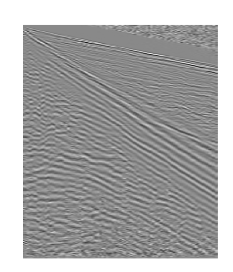
Figure 1: A space-time plot of seismic data. The horizontal axis represents the offset distance and the vertical axis indicates time. The origin is at the upper-left corner, and the maximum offset and time are 475 m and 1000 ms, respectively. The gray scale is such that black (white) corresponds to the minimum (maximum) amplitude of the seismic signal. The ground roll noise appears as downward oblique lines.

Figure 2: Seismic signal recorded by a single geophone (trace 58). The amplitude is in arbitrary units and time in ms.

Standard methods for suppressing ground roll include one-dimensional high–pass filtering and two-dimensional $f$–$k$ filtering Yilmaz (1987). Such “global” filters are based on the elimination of specific frequencies and have the disadvantage that they also affect the uncontaminated part of the signal. Recently, “local” filters for suppressing the ground roll have been proposed using the Karhunen-Loève transform Liu (1999); Tyapkin et al. (2004) and the wavelet transform Deighan and Watts (1997); Corso et al. (2003). The Wiener-Levinson algorithm has also been applied to extract the ground roll Karsli and Bayrak (2004).

Filters based on the Karhunen–Loève (KL) transform are particularly interesting because of the adaptativity of the KL expansion, meaning that the original signal is decomposed in a basis that is obtained directly from the empirical data, unlike Fourier and wavelet transforms which use prescribed basis functions. The KL transform is a mathematical procedure (also known as proper orthogonal decomposition, empirical orthogonal function decomposition, principal component analysis, and singular value decomposition) whereby any complicated data set can be optimally decomposed into a finite, and often small, number of modes (called proper orthogonal modes, empirical orthogonal functions, principal components or eigenimages) which are obtained from the eigenvectors of the data autocorrelation matrix. In applying the KL transform to suppress the ground roll, one must first map the contaminated region of the seismic record into a horizontal rectangular region. This transformed region is then decomposed with the KL transform and the first few principal components are removed to extract the coherent noise, after which the filtered data is inversely mapped back into the original seismic section. The advantage of this method is that the noise is suppressed with negligible distortion of the reflection signals, for only the data within the selected region is actually processed by the filter. Earlier versions of the KL filter Liu (1999); Tyapkin et al. (2004) have however one serious drawback, namely, the fact that the region to be filtered must be picked by hand—a procedure that not only can be labor intensive but also relies on good judgment of the person performing the filtering.

In this article we propose a significant improvement of the KL filtering method, in which the region to be filtered is selected automatically as an optimization procedure. We introduce a novel quantity, namely, the coherence index $CI$, which gives a measure of the amount of energy contained in the most coherent modes for a given selected region. The optimal region is then chosen as that that gives the maximum $CI$. We emphasize that introducing a quantitative criterion for selecting the ‘best’ region to be filtered has the considerable advantage of yielding a largely unsupervised scheme for demarcating and efficiently suppressing the ground roll.

Although our main motivation here concerns the suppression of coherent noise in seismic data, we should like to remark that our method may be applicable to other problems where coherent structures embedded in a complex spatiotemporal dynamics need to be identified or characterized in a more refined way. For example, the KL transform has been recently used to identify and extract spatial features from a complex spatiotemporal evolution in combustion experiment Palacios et al. (1998); Gorman et al. (2004); Blomgren et al. (2005). A related method—the so-called biorthogonal decomposition—has also been applied to characterize spatiotemporal chaos and identified structuresBouzat et al. (2004); Mininni et al. (2002) as well as identify changes in the dynamical complexity, and the spatial coherence of a multimode laser Papoff and D’Alessandro (2004). We thus envision that our optimized KL filter may find applications in these and related problems of coherent structures in complex spatiotemporal dynamics.

The article is organized as follows. In Sec. II we define the Karhunen–Loève transform, describe its main properties, and discuss its relation to the singular value decomposition of matrices. In Sec. III we present the KL filter and a novel optimization procedure to select the noise-contaminated region to be parsed through the filter. The results of our optimized filter when applied to the data shown in Fig. 1 are presented in Sec. IV. Our main conclusions are summarized in Sec. V. In Appendixes A and B we briefly discuss, for completeness, the relation between the KL transform and two other similar procedures known as proper orthogonal decomposition (or empirical orthogonal function expansion) and principal component analysis.

II The Karhunen–Loève Transform

II.1 Definition and main properties

Consider a multichannel seismic data consisting of $m$ traces with $n$ samples per trace represented by a $m\times n$ matrix $A$, so that the element $A_{ij}$ of the data matrix corresponds to the amplitude registered at the $i$th geophone at time $j$. For definiteness, let us assume that $m<n$, as is usually the case. We also assume for simplicity that the matrix $A$ has full rank, i.e., $r=m$, where $r$ denotes the rank of $A$. Letting the vectors $\vec{x}_{i}$ and $\vec{y}_{j}$ denote the elements of the $i$th row and the $j$th column of $A$, respectively, we can write

$$A=\left(\vec{y}_{1}\ \vec{y}_{2}\ ...\ \vec{y}_{n}\right)=\left(\begin{array}[]{c}\vec{x}_{1}\cr\vec{x}_{2}\cr...\cr\vec{x}_{m}\end{array}\right).$$ (1)

With the above notation we have

$$A_{ij}=x_{ij}=y_{ji},$$ (2)

where $a_{ij}$ denotes the $j$th element of the vector $\vec{a}_{i}$. (To avoid risk of confusion matrix elements will always be denoted by capital letters, so that a small-cap symbol with two subscripts indicates vector elements.)

Next consider the following $m\times m$ symmetric matrix

$$\Gamma\equiv AA^{t},$$ (3)

where the superscript $t$ denotes matrix transposition. It is a well known fact from linear algebra that matrices of the form (3), also called covariance matrices, are positive definite . Let us then arrange the eigenvalues $\lambda_{i}$ of $\Gamma$ in non-ascending order, i.e., $\lambda_{1}\geq\lambda_{2}\geq...\geq\lambda_{m}>0$, and let $\vec{u}_{i}$ be the corresponding (normalized) eigenvectors.

The Karhunen-Loève (KL) transform of the data matrix $A$ is defined as the $m\times n$ matrix $\Psi$ given by

$$\Psi=U^{t}A,$$ (4)

where the columns of the matrix $U$ are the eigenvectors of $\Gamma$:

$$U=\left(\vec{u}_{1}\ \vec{u}_{2}\ ...\ \vec{u}_{m}\right).$$ (5)

The original data can be recovered from the KL transform $\Psi$ by the inverse relation

$$A=U\Psi.$$ (6)

We refer to this equation as the KL expansion of the data matrix $A$. To render such an expansion more explicit let us denote by the $\vec{\chi}_{i}$, $i=1,...,m$, the elements of the $i$th row of the KL matrix $\Psi$, that is,

$$\Psi=\left(\begin{array}[]{c}\vec{\chi}_{1}\cr\vec{\chi}_{2}\cr...\cr\vec{\chi}_{m}\end{array}\right).$$ (7)

Then (6) can be written as

$$A=\sum_{i=1}^{m}\vec{u}_{i}\vec{\chi}_{i},$$ (8)

where it is implied matrix multiplication between the column vector $\vec{u}_{i}$ and the row vector $\vec{\chi}_{i}$. The eigenvectors $\vec{u}_{i}$ are called empirical eigenvectors, proper orthogonal modes, or KL modes.

As discussed in Appendix A, the total energy $E$ of the data can be defined as the sum of all eigenvalues,

$$E=\sum_{i=i}^{m}\lambda_{i},$$ (9)

so that $\lambda_{i}$ can be interpreted as the energy captured by the $i$th empirical eigenvector $\vec{u}_{i}$. We thus define the relative energy $E_{i}$ in the $i$th KL mode as

$$E_{i}=\frac{\lambda_{i}}{\sum_{i=i}^{m}\lambda_{i}}.$$ (10)

We note furthermore that since $\Gamma$ is a covariance-like matrix its eigenvalues $\lambda_{i}$ can also be interpreted as the variance of the respective principal component $\vec{u}_{i}$; see Appendix B for more details on this interpretation. We thus say that the higher $\lambda_{i}$ the more coherent the KL mode $\vec{u}_{i}$ is. In this context, the most energetic modes are identified with the most coherent ones and vice-versa.

An important property of the KL expansion is that it is ‘optimal’ in the following sense: if we form the matrix $\Psi_{k}$ by keeping the first $k$ rows of $\Psi$ and setting the remaining $m-k$ rows to zero, then the matrix $A_{k}$ given by

$$A_{k}=U\Psi_{k}$$ (11)

is the best approximation to $A$ by a matrix of rank $k<m$ in the Frobenius norm (the square root of the sum of the squares of all matrix elements) Holmes et al. (1996). This optimality property of the KL expansion lies at the heart of its applications in data compression Andrews et al. (1967) and dimensionality reduction Holmes et al. (1996), for it allows to approximate the original data $A$ by a smaller matrix $A_{k}$ with minimum loss of information (in the above sense). Another interpretation of relation (11) is that it gives a low-lass filter Freire and Ulrych (1988), for in this case only the first $k$ KL modes are retained in the filtered data $A_{k}$.

On the other hand, if the relevant signal in the application at hand is contaminated with coherent noise, as is the case of the ground roll in seismic data, one can use the KL transform to remove efficiently such noise by constructing a high-pass filter. Indeed, if we form the matrix $\Psi^{\prime}_{k}$ by setting to zero the first $k$ rows of $\Psi$ and keeping the remaining ones, then the matrix ${A^{\prime}}_{k}$ given by

$$A^{\prime}_{k}=U\Psi^{\prime}_{k}$$ (12)

is a filtered version of $A$ where the first $k$ ‘most coherent’ modes have been removed. However, if the noise is localized in space and time it is best to apply the filter only to the contaminated part of the signal. In previous versions of the KL filter the choice of the region to be parsed through the filter was made a priori, according to the best judgement of the person carrying out the filtering, thus lending a considerable degree of subjectivity to the process. In the next section, we will show how one can use the KL expansion to implement an automated filter where the undesirable coherent structure can be ‘optimally’ identified and removed.

Before going into that, however, we shall briefly discuss below an important connection between the KL transform and an analogous mathematical procedure known as the singular value decomposition of matrices. Readers already knowledgeable about the equivalence between these two formalisms (or more interested in the specific application of the KL transform to filter coherent noise) may skip the remainder of this section without loss of continuity.

II.2 Relation to Singular Value Decomposition

We recall that the singular value decomposition (SVD) of any $m\times n$ matrix $A$, with $m<n$, is given by the following expression:

$$A=U\Sigma V^{t},$$ (13)

where $U$ is as defined in (5), $\Sigma$ is a $m\times m$ diagonal matrix with elements $\sigma_{i}=\sqrt{\lambda_{i}}$, the so-called singular values of $A$, and $V$ is a $m\times n$ matrix whose columns correspond to the $m$ eigenvectors $\{\vec{v}_{i}\}$ of the matrix $A^{t}A$ with nonzero eigenvalues. The SVD allows us to rewrite the matrix $A$ as a sum of matrices of unitary rank:

$$A=\sum_{i=1}^{m}\sigma_{i}Q_{i}=\sum_{i=1}^{m}\sigma_{i}\vec{u}_{i}\vec{v}_{i}^{~{}t}.$$ (14)

In the context of image processing the matrices $Q_{i}$ are called eigenimages Andrews and Hunt (1977).

Now, comparing (6) with (13) we see that the KL transform $\Psi$ is related to the SVD matrices $\Sigma$ and $V$ by the following relation

$$\Psi=\Sigma V^{t},$$ (15)

so that the row vectors $\vec{\chi}_{i}$ of $\Psi$ are given in terms of the singular values $\sigma_{i}$ and the vectors $\vec{v}_{i}$ by

$$\vec{\chi}_{i}=\sigma_{i}\vec{v}_{i}^{~{}t}.$$ (16)

It thus follows that the decomposition in eigenimages seen in (14) is precisely the KL expansion given in (8). Furthermore the approximation $A_{k}$ given in (11) can be written in terms of eigenimages as

$$A_{k}=\sum_{i=1}^{k}\sigma_{i}Q_{i}.$$ (17)

Similarly, the filtered data $A^{\prime}_{k}$ shown in (12) reads in terms of eigenimages:

$$A^{\prime}_{k}=\sum_{i=k+1}^{m}\sigma_{i}Q_{i}.$$ (18)

The SVD provides an efficient way to compute the KL transform, and we shall use this method in the numerical procedures described in the paper.

III The Optimized KL Filter

Figure 3: Schematic diagram for demarcating the ground roll on a seismic section and the corresponding rectangular sectors obtained by applying a linear map.

As already mentioned, owing to its dispersive nature the ground-roll noise appears in a seismic image as a typical fan-like coherent structure. This space-time localization of the ground roll allows us to apply a sort of ‘surgical procedure’ to suppress the noise, leaving intact the uncontaminated region. To do that, we first pick lines to demarcate the start and end of the ground roll and, if necessary, intermediate lines to demarcate different wavetrains, as indicated schematically in Fig. 3. In this figure we have for simplicity used straight lines to demarcate the sectors but more general alignment functions, such as segmented straight lines, can also be chosen Liu (1999); Tyapkin et al. (2004). To make our discussion as general as possible, let us assume that we have a set of $N$ parameters $\{\theta_{i}\}$, $i=1,...,N$, describing our alignment functions. For instance, in Fig. 3 the parameters $\{\theta_{i}\}$ would correspond to the coefficients of the straight lines defining each sector.

Once the region contaminated by the ground roll has been demarcated, we map each sector onto a horizontal rectangular region by shifting and stretching along the time axis; see Fig. 3. The data points between the top and bottom lines in each sector is mapped into the corresponding new rectangular domain, with the mapping being carried out via a cubic convolution interpolation technique Park and Schowengerdt (1983). After this alignment procedure the ground roll events will become approximately horizontal, favoring its decomposition in a smaller space. Since any given transformed sector has a rectangular shape it can be represented by a matrix, which in turn can be decomposed in empirical orthogonal modes (eigenimages) using the KL transform. The first few modes, which contain most of the ground roll, are then subtracted to extract the coherent noise. The resulting data for each transformed sector is finally subjected to the corresponding inverse mapping to compensate for the original forward mapping. This leaves the uncontaminated data (lying outside the demarcated sectors) unaffected by the whole filtering procedure.

The KL filter described above has indeed shown good performance in suppressing source-generated noise from seismic data Liu (1999); Tyapkin et al. (2004). The method has however the drawback that the region to be filtered must be picked by hand, which renders the analysis somewhat subjective. In order to overcome this difficulty, it would be desirable to have a quantitative criterion based on which one could decide what is the ‘best choice’ for the parameters $\{\theta_{i}\}$ describing the alignment functions. In what follows, we propose an optimization procedure whereby the region to be filtered can be selected automatically, once the generic form of the alignment functions is prescribed.

Suppose we have chosen $l$ sectors to demarcate the different wavetrains in the contaminated region of the original data, and let $\{\theta_{1},...,\theta_{N}\}$ be the set of parameters characterizing the respective alignment functions that define these sectors. Let us denote by $\tilde{A}_{k}$, $k=1,...,l$, the matrix representing the $k$th transformed sector obtained from the linear mapping of the respective original sector, as discussed above. For each transformed sector $\tilde{A}_{k}$ we then compute its KL transform and calculate the coherence index $CI_{k}$ for this sector, defined as the relative energy contained in its first KL mode:

$$CI_{k}=\frac{\lambda_{1}^{k}}{\sum_{i=1}^{r_{k}}\lambda_{i}^{k}},$$ (19)

where $\lambda_{i}^{k}$ are the eigenvalues of the correlation matrix $\tilde{\Gamma}_{k}=\tilde{A}_{k}\tilde{A}^{t}_{k}$ and $r_{k}$ is the rank of $\tilde{A}_{k}$. Such as defined above, $CI_{k}$ represents the relative weight of the most coherent mode in the KL expansion of the transformed sector $\tilde{A}_{k}$. (A quantity analogous to our $CI$ is known in the oceanography literature as the similarity index Kim et al. (2002).)

Next we introduce an overall coherence index $CI(\theta_{1},...,\theta_{N})$ for the entire demarcated region, defined as the average coherence index of all sectors:

$$CI(\theta_{1},...,\theta_{N})=\frac{1}{l}{\sum_{k=1}^{l}CI_{k}}.$$ (20)

As the name suggests, the coherence index $CI$ is a measure of the amount of ‘coherent energy’ contained in the chosen demarcated region given by the parameters $\{\theta_{i}\}_{i=1}^{N}$. Thus, the higher $CI$ the larger the energy contained in the most coherent modes in that region. For the purpose of filtering coherent noise it is therefore mostly favorable to pick the region with the largest possible $CI$. We thus propose the following criterion to select the optimal region to be filtered: vary the parameters $\{\theta_{i}\}$ over some appropriate range and then choose the values $\theta_{i}^{*}$ that maximize the coherence index $CI$, that is,

$$CI(\theta_{1}^{*},...,\theta_{N}^{*})=\max_{\{\theta_{i}\}}\left[CI(\theta_{1},...,\theta_{N})\right].$$ (21)

Once we have selected the optimal region, given by the parameters $\{\theta_{i}^{*}\}_{i=1}^{N}$, we then simply apply the KL filter to this region as already discussed: we remove the first few eigenimages from each transformed sector and inversely map the data back into the original sectors, so as to obtain the final filtered image. In the next section we will apply our optimized KL filtering procedure to the seismic data shown in Fig. 1.

IV Results

Here we illustrate how our optimized KL filter works by applying it to the seismic data shown in Fig. 1. In this case, it suffices to choose only one sector to demarcate the entire region contaminated by the ground roll. This means that we have to prescribe only two alignment functions, corresponding to the uppermost and lowermost straight lines (lines AB and CD, respectively) in Fig. 3. To reduce further the number of free parameters in the problem, let us keep the leftmost point of the upper line (point A in Fig. 3) fixed to the origin, so that the coordinates $(i_{A},j_{A})$ of point A are set to $(0,0)$, while allowing the point $B$ to move freely up or down within certain range; see below. Similarly, we shall keep the rightmost point of the lower line (point C in Fig. 3) pinned at a point $(i_{C},j_{C})$, where $i_{C}=95$ and $j_{C}$ is chosen so that the entire ground roll wavetrain is above this point. The other endpoint of the lower demarcation line (point $D$ in Fig. 3) is allowed to vary freely. With such restrictions, we are left with only two free parameters, namely, the angles $\theta_{1}$ and $\theta_{2}$ that the upper and lower demarcation lines make with the horizontal axis. So reducing the dimensionality of our parameter space allows us to visualize the coherence index $CI(\theta_{1},\theta_{2})$ as a 2D surface. For the case in hand, it is more convenient however to express $CI$ not as a function of the angles $\theta_{1}$ and $\theta_{2}$ but in terms of two other new parameters introduced below.

Let the coordinates of point $B$, which defines the right endpoint of the upper demarcation line in Fig. 3, be given by $(i_{B},j_{B})$, where $i_{B}=95$. In our optimization procedure we let point $B$ move along the right edge of the seismic section by allowing the coordinate $j_{B}$ to vary from a minimum value $j_{B_{min}}$ to a maximum value $j_{B_{max}}$, so that we can write

$$j_{B}=j_{B_{min}}+k\Delta_{B},\quad k=0,1,...,N_{B}$$ (22)

where $N_{B}$ is the number of intermediate sampling points between $j_{B_{min}}$ and $j_{B_{max}}$, and $\Delta_{B}=(j_{B_{max}}-j_{B_{min}})/N_{B}$. Similarly, for the coordinates $(i_{D},j_{D})$ of point $D$ in Fig. 3, which is the moving endpoint of the lower straight line, we have $i_{D}=0$ and

$$j_{D}=j_{D_{min}}+l\Delta_{D},\quad l=0,1,...,N_{D},$$ (23)

where $N_{D}$ is the number of sampling points between $j_{D_{min}}$ and $j_{D_{max}}$, and $\Delta_{D}=(j_{D_{max}}-j_{D_{min}})/N_{D}$.

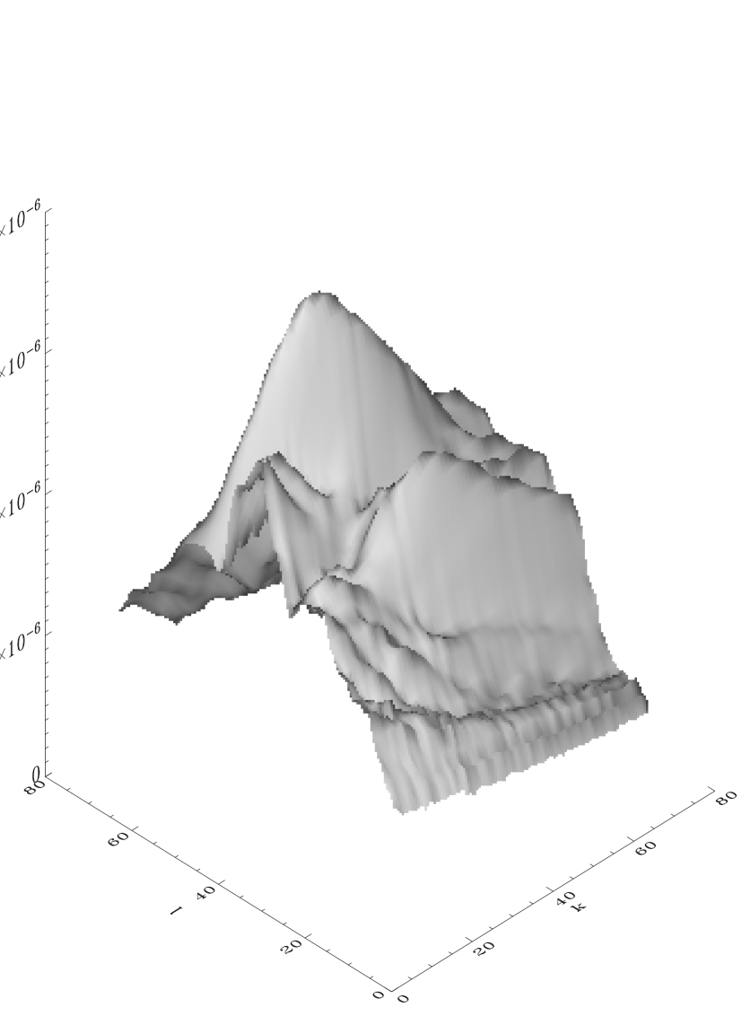
Figure 4: The coherence index $CI$ as a function of the indices $k$ and $l$ that define the demarcation lines; see text.

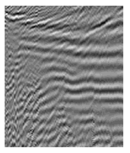
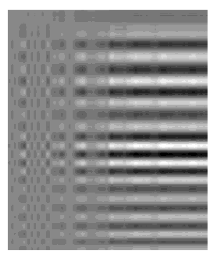
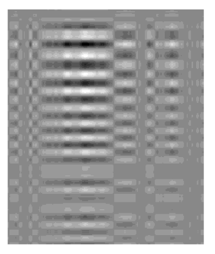
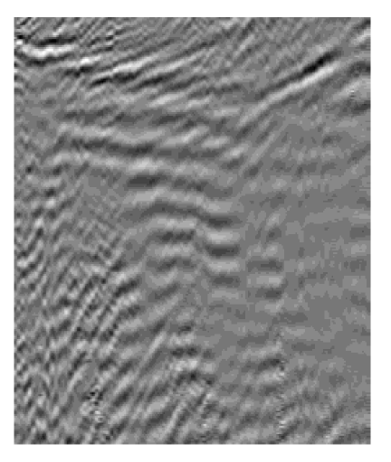
Figure 5: a) The selected region in the new domain; b) its first eigenimage; c) the second eigenimage; and d) the result after subtracting the first eigenimage.

For each choice of $k$ and $l$ in (22) and (23), we apply the procedure described in the previous section and obtain the coherence index $CI(k,l)$ of the corresponding region. In Fig. 4 we show the energy surface $CI(k,l)$, for the case in which $j_{B_{min}}=280$, $j_{B_{max}}=600$, $j_{C}=864$, $j_{D_{min}}=0$, $j_{D_{max}}=576$, and $N_{B}=N_{D}=64$. We see in this figure that $CI$ possesses a sharp peak, thus showing that this criterion is indeed quite discriminating with respect to the positioning of the lines demarcating the region contaminated by the ground roll. The global maximum of $CI$ in Fig. 4 is located at $k=42$ and $l=24$, and in Fig. 5a we show the transformed sector obtained from the linear mapping of this optimal region. In this figure one clearly sees that the ground roll wavetrains appear mostly as horizontal events. In Fig. 5b we present the first eigenimage of the data shown in Fig. 5a, which corresponds to about 33% of the total energy of the image in Fig. 5a, as can be seen in Fig. 6 where we plot the relative energy $E_{i}$ captured by the first 10 eigenimages. The second eigenimage, shown in Fig. 5c, captures about 10% of the total energy, with each successively higher mode contributing successively less to the total energy; see Fig. 6. In Fig. 5d we give the result of removing the first KL mode (Fig. 5b) from Fig. 5a. It is clear in Fig. 5d that by removing only the first eigenimage the main horizontal events (corresponding to the ground roll) have already been greatly suppressed.

Performing the inverse mapping of the image shown in Fig. 5c yields the data seen in the region between the two white lines in Fig. 7a, which shows the final filtered image for this case (i.e., after removing the first KL mode from the transformed region). We see that the ground roll inside the demarcated region in Fig. 7a has been considerably suppressed, while the uncontaminated signal (lying outside the marked region) has not been affected at all by the filtering procedure. If one wishes to filter further the ground roll noise one may subtract successively higher modes. For example, in Fig. 7b we show the filtered image after we also subtract the second eigenimage. One sees that there is some minor improvement, but removing additional modes is not recommended for it starts to degrade relevant signal as well.

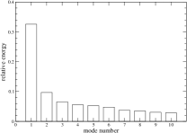
Figure 6: The relative energy of the first 10 KL modes of the region shown in Fig. 5a.

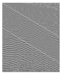
Figure 7: a) The filtered seismic section after removing the first eigenimage of the select region shown in Fig. 5a. In b) we show the result after removing the first two eigenimages.

V Conclusions

An optimized filter based on the Karhunen–Loéve transform has been constructed for processing seismic data contaminated with coherent noise (ground roll). A great advantage of the KL filter lies in its local nature, meaning that only the contaminated region of the seismic record is processed by the filter, which allows the ground roll to be removed without distorting most of the reflection signal. Another advantage is that it is an adaptative method in the sense the the signal is decomposed in an empirical basis obtained from the data itself. We have improved considerably the KL filter by introducing an optimization procedure whereby the ground roll region is selected so as to maximize an appropriately defined coherence index $CI$. We emphasize that our method, require as input, only the generic alignment functions to be used in the optimization procedure as well as the number of eigenimages to be removed from the selected region. These may vary depending on the specific application at hand. However, once these choices are made, the filtering task can proceed in the computer in an automated way.

Although our main motivation here has been suppressing coherent noise from seismic data, our method is by no means restricted to geophysical applications. In fact, we believe that the method may prove useful in other problems in physics that require localizing coherent structures in an automated and more refined way. We are currently exploring further such possibilities.

Appendix A Relation between the KL transform and Proper Orthogonal Decomposition

In dynamical systems the mathematical procedure akin to the KL transform is called the proper orthogonal decomposition (POD). In this context, one may view each column vector $\vec{y}_{j}$ of the data matrix $A$ as a set of $m$ measurements (real or numerical) of a given physical variable $f(x,t)$ performed simultaneously at $m$ space locations and at a certain time $t_{j}$, that is, $y_{jk}=f(x=x_{k},t=t_{j})$, $k=1,...,m$. For example, in turbulent flows the vectors $\vec{y}_{i}$ often represent measurements of the fluid velocity at $m$ points in space at a given time $i$. The data matrix $A$ thus corresponds to an ensemble $\{\vec{y}_{j}\}$ of $n$ such vectors, representing a sequence of $m$ measurements over $n$ instants of time. In POD one is usually concerned with finding a low-dimensional approximate description of the high-dimensional dynamical process at hand. This is done by finding an ‘optimal’ basis in which to expand (and then truncate) a typical vector $\vec{y}$ of the data ensemble. Such a basis is given by the eigenvectors of the time-averaged autocorrelation matrix $R$, which is proportional to the matrix $\Gamma$ define above:

$$R\equiv\left<\vec{y}\,\vec{y}^{\;t}\right>=\frac{1}{n}\sum_{i=1}^{n}\vec{y}_{i}\,\vec{y}_{i}^{\,t}=\frac{1}{n}\Gamma.$$ (24)

Hence the eigenvectors $\{\vec{u}_{i}\}$ of $\Gamma$ are also eigenvectors of $R$. In POD parlance the eigenvectors $\{\vec{u}_{i}\}$ are called empirical eigenvectors or proper orthogonal modes. In the continuous case, the corresponding eigenfunctions $u_{i}(x)$ of the autocorrelation operator are known as empirical orthogonal functions (EOF).

From (1), (4) and (5), one can easily verify that

$$\Psi_{ij}=\vec{u}_{i}\cdot\vec{y}_{j}.$$ (25)

We thus see that the columns of the KL transform $\Psi$ correspond to the coordinates of the vectors $\vec{y}$ in the empirical basis:

$$\vec{y}_{i}=\sum_{k=1}^{m}\Psi_{ki}\vec{u}_{k}.$$ (26)

It is this expansion of any member of the ensemble in the empirical basis that is called the proper orthogonal decomposition or empirical orthogonal function expansion. It now follows from (26) that

$$\left<\vec{y}^{\;2}\right>=\frac{1}{n}\sum_{i=1}^{n}\vec{y}_{i}^{\;2}=\frac{1}{n}\sum_{i}(\Psi\Psi^{t})_{ii}=\frac{1}{n}\sum_{i}\lambda_{i},$$ (27)

where in the last equality we used the fact that

$$\Psi\Psi^{t}=U^{t}\Gamma U=\Lambda,$$ (28)

where $\Lambda$ is the diagonal matrix $\Lambda={\rm diag}(\lambda_{1},...,\lambda_{m})$. Equation (27) thus suggests that we can interpret the eigenvalue $\lambda_{i}$ as a measure of the energy in the $i$th empirical orthogonal mode. For example, in the case of turbulent flows where the vector $\vec{y}_{i}$ contains velocity measurements at time $i$, the left hand of (27) yields twice the average kinetic energy per unit mass, so that $\frac{1}{2}\lambda_{i}$ gives the kinetic energy in the $i$th empirical orthogonal mode Holmes et al. (1996). Similarly, in the case of seismic data the vectors $\vec{y}_{i}$ represent amplitudes of the reflected waves, and hence the quantity $\sum_{i=1}^{n}\vec{y}_{i}^{\;2}=\sum_{i=i}^{n}\lambda_{i}$ may be viewed as a measure of the total energy of the data, thus justifying the definition given in (9).

The optimality of the KL expansion also has a nice physical and geometrical interpretation, as follows. Suppose we write a vector $\vec{y}$ in an arbitrary orthonormal basis $\{\vec{e}_{i}\}_{i=1}^{m}$:

$$\vec{y}=\sum_{i=1}^{m}a_{i}\vec{e}_{i},$$ (29)

where $a_{i}=\vec{e}_{i}\cdot\vec{y}$. If we now wish to approximate $\vec{y}$ by only its first $k<m$ components,

$$\vec{y}^{\,k}=\sum_{i=1}^{k}a_{i}\vec{e}_{i},$$ (30)

then the optimality of the KL expansion implies that the first $k$ proper orthogonal modes capture more energy (on average) that the first $k$ modes of any other basis. More precisely, the mean square distance $\left<|\vec{y}-\vec{y}^{\,k}|^{2}\right>$ is minimum if we use the empirical basis.

Appendix B Relation between the KL transform and Principal Component Analysis

In statistical analysis of multivariate data, the KL transform is known as principal component analysis (PCA). In this case, one views the elements of a row vector $\vec{x}_{i}=(x_{i1},...,x_{in})$ of the data matrix $A$ as being $n$ realizations of a random variable $X_{i}$, so that the matrix $A$ itself corresponds to $n$ samples of a random vector $\vec{X}$ with $m$ components: $\vec{X}=(X_{1},...,X_{m})^{t}$. In other words, the column vectors $\vec{y}_{j}$ correspond to the samples of $\vec{X}$. If the rows of $A$ are centered, i.e., the variables $X_{i}$ have zero mean, then the matrix $\Gamma$ is proportional to the covariance matrix $S_{X}$ of $\vec{X}$ :

$$({S_{X}})_{ij}\equiv\left<X_{i}X_{j}\right>=\frac{1}{n}\vec{x_{i}}\cdot\vec{x_{j}}=\frac{1}{n}\Gamma_{ij},$$ (31)

or alternatively in matrix notation

$$S_{X}\equiv\left<\vec{X}\,\vec{X}^{\;t}\right>=\frac{1}{n}\Gamma.$$ (32)

[Note that the matrices $R$ and $S_{X}$ defined respectively in (24) and (32) are essentially the same but have different interpretations.] In the PCA context, the diagonal elements $\Gamma_{ii}$ of the matrix $\Gamma$ are thus proportional to the variance of the variables $X_{i}$, whereas the off-diagonal elements $\Gamma_{ij}$, $i\neq j$, are proportional to the covariance between the variables $X_{i}$ and $X_{j}$. Furthermore, the eigenvectors $\vec{u}_{i}$ of $\Gamma$ correspond to the principal axis of the covariance matrix $S_{X}$. The idea behind PCA is to introduce a new set of $m$ variables $P_{i}$, each of which being a linear combination of the original variables $X_{i}$, such that these new variables are mutually uncorrelated. This is accomplished by projecting the vector $\vec{X}$ onto the principal directions of the covariance matrix. More precisely, we define the principal components $P_{i}$, $i=1,...,m$, by the following relation

$$P_{i}=\vec{X}\cdot\vec{u}_{i}=\sum_{j=1}^{n}u_{ij}X_{j}.$$ (33)

In other words, the vector of principal components $\vec{P}=(P_{1},...,P_{m})^{t}$ is obtained from a rotation of the original vector $\vec{X}$:

$$\vec{P}=U^{t}\vec{X}.$$ (34)

The covariance matrix $S_{P}$ of the principal components is then given by

$$S_{P}=\left<\vec{P}\,\vec{P}^{\,t}\right>=\left<U^{t}\vec{X}\,\vec{X}^{\,t}U\right>=\frac{1}{n}U^{t}\Gamma U=\frac{1}{n}\Lambda,$$ (35)

thus showing that

$$\left<P_{i}P_{j}\right>=0,\quad{\rm for}\quad i\neq j,$$ (36)

as desired. The first principal component $P_{1}$ then represents the particular linear combination of the original variables $X_{i}$ (among all possible such combinations that yield mutually uncorrelated variables) that has the largest variance, with the second principal component possessing the second largest variance, and so on.

From (4) and (34) one sees that the elements of the $i$th row of the KL transform $\Psi$ correspond to the $n$ samples or scores of the $i$th principal component. That is, if we denote the sample vector of the $i$th principal component by $\vec{p}_{i}=(p_{i1},...,p_{in})$, then $p_{ij}=\vec{u}_{i}\cdot\vec{y}_{j}=\Psi_{ij}$. For this reason in the PCA context the KL transform $\Psi$ is called the matrix of scores.

References

- Yilmaz (1987) O. Yilmaz, Seismic Data Processing (Society of Exploration Geophysicist, Tulsa, 1987).
- Liu (1999) X. Liu, Geophysics 64, 564 (1999).
- Tyapkin et al. (2004) Y. K. Tyapkin, N. Marmalevskyy, and Z. V. Gornyak, in EAGE 66th Conference (2004), expanded Abstract D028.
- Deighan and Watts (1997) A. J. Deighan and D. R. Watts, Geophysics 62, 1896 (1997).
- Corso et al. (2003) G. Corso, P. Kuhn, L. Lucena, and Z. Thomé, Physica A 318, 551 (2003).
- Karsli and Bayrak (2004) H. Karsli and Y. Bayrak, Journal of Applied Geophysics 55, 187 (2004).
- Palacios et al. (1998) A. Palacios, G. H. Gunaratne, M. Gorman, and K. A. Robbins, Phys. Rev. E 57, 5958 (1998).
- Gorman et al. (2004) K. R. M. Gorman, J. Bowers, and R. Brockman, Chaos 14, 467 (2004).
- Blomgren et al. (2005) P. Blomgren, S. Gasner, and A. Palacios, Chaos 15, 013706 (2005).
- Bouzat et al. (2004) S. Bouzat, H. S. Wio, and G. B. Mindlin, Physica D 199, 185 (2004).
- Mininni et al. (2002) P. D. Mininni, D. O. Gómez, and G. B. Mindlin, Phys. Rev. Lett. 89, 061101 (2002).
- Papoff and D’Alessandro (2004) F. Papoff and G. D’Alessandro, Phys. Rev. A 70, 063805 (2004).
- Holmes et al. (1996) P. Holmes, J. L. Lumley, and G. Berkooz, Turbulence,Coherent Structures, Dynamical Systems and Symmetry (Cambridge University Press, Cambridge, 1996).
- Andrews et al. (1967) C. Andrews, J. Davies, and G. Schwartz, Proc. IEEE 55, 267 (1967).
- Freire and Ulrych (1988) S. Freire and T. Ulrych, Geophysics 53, 778 (1988).
- Andrews and Hunt (1977) H. Andrews and B. Hunt, Digital Image Restoration (Prentice Hall, 1977).
- Park and Schowengerdt (1983) S. Park and R. Schowengerdt, Computer, Vision, Graphics & Image Processing 23, 256 (1983).
- Kim et al. (2002) H.-J. Kim, J.-K. Chang, H.-T. Jou, G.-T. Park, B.-C. Suk, and K. Y. Kim, J. Acoust. Soc. Am. 111, 794 (2002).