Noise-induced clustering in Hamiltonian systems

Abstract

The motion of oscillatory-like nonlinear Hamiltonian systems, driven by a weak noise, is considered. A general method to find regions of stability in the phase space of a randomly-driven system, based on a specific Poincaré map, is proposed and justified. Physical manifestations of these regions of stability, the so-called coherent clusters, are demonstrated with two models in ocean physics. We find bunches of sound rays propagating coherently in an underwater waveguide through a randomly fluctuating ocean at long distances. We find clusters of passive particles to be advected coherently by a random two-dimensional flow modelling mixing around a topographic eddy in the ocean.

I Introduction

The interplay between dynamical chaos and noise is a topic of interest both in nonlinear dynamics and statistical physics. Real-world systems operate against a noisy background. Both chaos and noise mean random or diffusive-like behavior in the nonlinear system‘s dynamics that can be quantified by the maximal Lyapunov exponents

$$\lambda=\lim_{t\to\infty}\lambda(t),\qquad\lambda(t)=\lim_{\Delta(0)\to 0}\frac{1}{t}\ln\frac{\Delta(t)}{\Delta(0)},$$ (1)

where $\Delta(t)$ is a distance (in the Euclidean sense) in a direction at the moment $t$ between two initially closed trajectories.

However, the methods and approaches to study deterministic and random system are different. Typical deterministic nonlinear systems (the so-called nonhyperbolic system) are known to have mixed phase space with coexisting regions of stable and unstable motion. There are islands of regular motion merged into a chaotic sea, islands around islands, stochastic layers confined between invariant tori, cantory nearby the boundaries of islands, and so on (for a recent review of chaos in Hamiltonian systems see Z04 ). The motion is predictable in some regions but permits a statistical description only in those ones where extremal sensitivity to initial conditions takes place. The notion of the mixing time, the reciprocal maximal Lyapunov exponent, can be introduced to quantity the so-called predictability horizon.

To describe randomly-driven systems one uses some ergodic postulates based on the assumption of fully developed chaos. In Hamiltonian nonintegrable systems intermittent-like dynamics with chaotic oscillations interrupted by regular ones seems to be more realistic. It means, in particular, that regular motion does not cease suddenly, and completely stochastic motion does not arise suddenly just beyond the predictability horizon. Remnants of stability should persist for more long times. It is especially true for oscillatory-like systems due to resonant interaction of unperturbed motion with random perturbation MUP04 .

In this paper we treat a model of a randomly-driven nonlinear oscillator from purely deterministic point of view, and show that there are regions of stability surviving for a comparatively long time under a weak noisy excitation with arbitrary spectrum. This time can be estimated with the help of a specific map which plays the role of the Poincaré map in periodically-driven systems. The map is intended to find numerically clusters of trajectories with close initial conditions which are stable by Lyapunov with a given realization of the random perturbation (Sec. II). We check the effectiveness of the procedure proposed with two problems of ocean physics where, as in other geophysical problems, there is, as a rule, no respective statistical ensemble of averaging, and we deal with single realizations in the field experiments. Noise-induced coherent clusters are demonstated with the ray model of sound propagation in an ocean waveguide with a randomly fluctuating sound-speed profile induced by internal waves in the deep ocean (Sec. III). Another example is clustering of passive particles advected by a random two-dimensional velocity field in an ideal fluid (Sec. IV).

II Effective Poincaré map

In this section we introduce an effective Poincaré map that, like to the usual Poincaré map, enables to find numerically regions of stability in the phase space of a Hamiltonian system surviving under a weak random perturbation due to nonlinear resonances between the unperturbed motion and the perturbation.

Let us consider a one-dimensional nonlinear oscillator with the Hamoltonian

$$H=H_{0}+\varepsilon H_{1}(t)=\frac{p^{2}}{2}+U(q)+\varepsilon V(q)\xi(t),$$ (2)

where $q$ and $p$ are position and momentum, U(q) is an unperturbed potential, $V(q)$ is a smooth function, $\xi(t)$ is a weak noise with $\varepsilon\ll 1$, and normalized first and second moments, $\left<\xi\right>=0$ and $\left<\xi^{2}\right>=1/2$. Hereafter, we will consider a single realization of noise, $\xi(t)$, and, therefore, the equations of motion

$$\frac{dq}{dt}=p,\quad\frac{dp}{dt}=-\frac{dU}{dq}-\varepsilon\frac{dV}{dq}\xi(t),$$ (3)

can be treated as deterministic ones. Introducing the canonical transformation from the $(q,p)$ variables to the action–angle variables (see Z04 ; LL )

$$I=\frac{1}{2\pi}\oint p\,dq,\quad\vartheta=\frac{\partial}{\partial I}\int\limits_{q^{\prime}}^{q}p(q,\,H)\,dq,$$ (4)

we rewrite Eqs.(3) in the form

$$\frac{dI}{dt}=-\frac{\partial H(I,\,\vartheta)}{\partial\vartheta}=-\varepsilon\frac{\partial V(I,\,\vartheta)}{\partial\vartheta}\xi(t),$$ (5)

$$\frac{d\vartheta}{dt}=\frac{\partial H(I,\,\vartheta)}{\partial I}=\omega(I)+\varepsilon\frac{\partial V(I,\,\vartheta)}{\partial I}\xi(t),$$

where $\omega(I)\equiv\partial H_{0}/\partial I$ is an action-dependent characteristic frequency of oscillations.

The notion of stability means a weak sensitivity of a solution to small changes in initial conditions that is quantified by the Lyapunov exponent (1). As we know from KAM-theory AKN , most of the invariant tori of integrable Hamiltonian systems, where the motion is stable, are preserved under a small perturbation. In spite of each single realization of a random perturbation $\xi(t)$ can be treated as a deterministic function than a stochastic one, infinite number of frequencies in the spectrum of $\xi(t)$ leads to densely distributed resonances in the phase space and laking of invariant tori. In the limit $t\to\infty$, no regions in the phase space remain forbidden under a noisy perturbation. Even a weak noise can accelerate phase-space transport by forcing trajectories to traverse KAM tori C79 ; RRW81 ; LL . So deterministic description ceases to have a sense, and one forces to use statistical description of the motion.

However, in practics, we deal with a finite time interval $[0:T_{0}]$. Moreover, in geophysical field experiments experimentalists work mainly with single realizations of nonstationary processes of interest. By these reasons we can recover “deterministic” methods to explore the sets of stable trajectories satisfying to the condition of the finite-time invariance: if any set in the phase space at $t=0$ transforms to itself at $t=T_{0}$ without mixing, then it corresponds to an ensemble of trajectories which are stable by Lyapunov within the interval $[0:T_{0}]$. In order to find such stable sets for an arbitrary spectrum of perturbation, we propose the following map

$$\begin{array}[]{c}I_{i+1}=I(t=T_{0},\,I_{i},\vartheta_{i}),\quad\vartheta_{i+1}=\vartheta(t=T_{0},\,I_{i},\vartheta_{i}),\end{array}$$ (6)

where $I(t;\,I_{i},\vartheta_{i})$ and $\vartheta(t;\,I_{i},\vartheta_{i})$ are the solutions of Eqs.(5) with initial conditions $I(0)=I_{i}$, $\vartheta(0)=\vartheta_{i}$. In fact, this map is equivalent to a Poincaré map for a system with the Hamiltonian

$$H=H_{0}(I)+V(I,\,\vartheta)\tilde{\xi}(t),$$ (7)

where $\tilde{\xi}(t)$ is a periodic function consisting of identical pieces of $\xi(t)$ of the same duration $T_{0}$

$$\tilde{\xi}(t+nT_{0})=\xi(t),\quad 0\leq t\leq T_{0},\quad n=0,1,\dots.$$ (8)

In this way we replace our original randomly-driven system by a periodically-driven one. It should be emphasized that the validity of this replacement in restricted by the time interval $[0:T_{0}]$. By analogy with the usual Poincaré map, the key property of the map (6) is the following: each point of a continuous closed trajectory of the map (6) corresponds to a starting point of the solution of Eqs.(5) which remains stable by Lyapunov till the time $T_{0}$. The inverse statement is not, in general, true. It will be shown below that the map (6) provides sufficient but not necessary criterion of stability. Topological properties of trajectories of the map (6) can be treated in the framework of the theory of nonlinear resonance C79 . The functions $V(I,\,\vartheta)$ and $\tilde{\xi}(t)$ can be decomposed in Fourier series

$$V(I,\,\vartheta)=\sum\limits_{l=-\infty}^{\infty}V_{l}(I)\,\exp[i(l\vartheta+\phi_{l})],$$ (9)

$$\tilde{\xi}(t)=\sum\limits_{m=-\infty}^{\infty}\xi_{m}\,\exp[i(m\Omega t+\psi_{m})],$$

where $\Omega=2\pi/T_{0}$. The Fourier amplitudes of the analytic function $V$ decay as $V_{l}(I)\sim\exp(-\sigma l)$, whereas the ones for the random function $\xi(t)$ decay as $\xi_{m}\sim m^{-\beta}$ ($0\leq\beta\leq 1$ and $\beta=0$ for a white noise) since $\xi(0)\neq\xi(T_{0})$. If the interval $T_{0}$ is large enough, the parameter $\beta$ is determined mainly by the correlation time of $\xi(t)$.

Substituting the expansions (9) into the equations of motion (5) and omitting rapidly oscillating terms $\exp[i(l\vartheta+m\Omega t)]$, we get the following equations:

$$\frac{dI}{dt}=-\frac{i\varepsilon}{2}\sum\limits_{l,m=0}^{\infty}lV_{l}\xi_{m}\exp{i\Phi}+\text{c.\ c.},$$ (10)

$$\frac{d\vartheta}{dt}=\omega+\frac{\varepsilon}{2}\sum\limits_{l,m=0}^{\infty}\frac{\partial V_{l}}{\partial I}\xi_{m}\exp{i\Phi}+\text{c.\ c.},$$

where $\Phi=l\vartheta-m\Omega t+\phi_{l}-\psi_{m}$. The stationary phase condition $d\Phi/dt=0$ implies the resonances of the map (6)

$$mT(I)=lT_{0},$$ (11)

where $T(I)=2\pi/\omega(I)$ is a period of unperturbed oscillations with a given value of the action $I$. Resonant values of the action $I_{\text{res}}$ can be found from the condition (11). The relation $l:m$ defines the order of the respective resonance. It should be noted that an infinite number of resonances $jl:jm$ ($j=1,2,...$) corresponds simultaneously to each value of the resonant action. However, if $I_{\text{res}}$ is far enough from the separatrix value, the product $V_{l}\xi_{m}$ decreases rapidly with increasing $j$, and the resonances with small values of $l$ and $m$ only can affect significantly a trajectory. Thus, if $T_{0}>T(I_{\text{res}})$, only the superior term with $l=1$ should be taken into account. Neglecting the higher-order resonances, we can describe the motion in the vicinity of $I_{\text{res}}$ in the pendulum approximation C79 . Leaving the resonant term only, we can rewrite Eqs.(10) in the form

$$\frac{dI}{dt}=\varepsilon V_{1}(I_{\mathrm{res}})\xi_{m}\sin\Phi,$$ (12)

$$\frac{d\Phi}{dt}=\omega-m\Omega+\varepsilon\frac{\partial V_{1}(I_{\mathrm{res}})}{\partial I}\xi_{m}\cos\Phi,$$

which corresponds with some simplification to the universal Hamiltonian of nonlinear resonance C79 ; Z04

$$H_{u}=\frac{1}{2}\,\bigl{|}\omega^{\prime}_{I}\bigr{|}\left(\Delta I\right)^{2}+\varepsilon V_{l}\xi_{m}\cos{\Phi},$$ (13)

where $\Delta I=I-I_{\text{res}}$. Solutions of Eqs.(12) describe oscilations of the action $I$ and phase $\Phi$ variables nearby elliptic fixed points of the respective resonances, the so-called phase oscillations.

An angular location of the fixed points depends on a random phase $\psi_{m}$ and, therefore, varies from one realization of the random function $\xi(t)$ to another. A trajectory of the map (6), being captured into a resonance, draws a chain-like structure in the phase space. In the regime of stable motion neighboring chains are far enough from each other, and the space between them is filled by non-resonant stable trajectories. The width of the resonance in terms of the frequency can be estimated from the Hamiltonian (13) as follows:

$$\Delta\omega=|\omega^{\prime}_{I}|\Delta I_{\text{max}}\simeq 2\sqrt{\varepsilon|\omega^{\prime}_{I}|V_{1}\xi_{m}},$$ (14)

where $\omega^{\prime}_{I}=d\omega/dI$ is related to nonlinearity of oscillations and determined by the form of the unperturbed potential. The distance between the neighboring resonances of the successive orders is $\delta\omega(T_{0})=2\pi/T_{0}$. If the criterion of Chirikov, $\Delta\omega/\delta\omega\simeq 1$, holds, the resonances overlap in the phase space, and the phase oscillations become unstable.

Except for some specific situations, the Chirikov’s criterion provides a sufficient condition for emergence of global chaos. We can estimate from the above relations the time that is required for overlapping all the resonances in the phase space

$$T_{\text{c}}\simeq\frac{\pi}{\sqrt{\varepsilon|\omega^{\prime}_{I}|V_{1}(I_{\text{min}})\xi_{m}}},$$ (15)

where $I_{\text{min}}$ is a minimal resonant action corresponding to the deepest resonance, and the amplitudes $\xi_{m}$ are supposed to be independent on time. Nevertheless, some stable regions in the phase space can survive at $T>T_{\text{c}}$ in the form of islands submerged into a stochastic sea. The time horizon $T_{\text{c}}$ may be treated as a time of mixing in the phase space. With a given spectrum of noise and large enough values of $T_{0}$, difference between the amplitudes $\xi_{m}$ for different realizations of the noise becomes negligible. Therefore, the time of phase correlations $T_{\text{c}}$ is independent on the realization chosen and may be treated as a characteristic quantity of a Hamiltonian system under consideration.

III Clustering of sound rays in an ocean waveguide

Low-frequency acoustic signals may propagate in the deep ocean to very long ranges due to existence of the underwater sound channel which acts as a waveguide confining sound waves within a restricted water volume (see general theory in Ref. BL91 and description of field experiments in the Pacific ocean in the issue JASA ). In the geometric optics approximation, the underwater sound ray trajectories in a two-dimensional waveguide in the deep ocean with the sound speed $c$, being a smooth function of depth $z$ and range $r$, satisfy the canonical Hamiltonian equations LaL

$$\frac{dz}{dr}=\frac{\partial H}{\partial p},\qquad\frac{dp}{dr}=-\frac{\partial H}{\partial z},$$ (16)

with the Hamiltonian

$$H=-\sqrt{n^{2}(z,r)-p^{2}},$$ (17)

where $n(z,r)=c_{0}/c(z,r)$ is the refractive index, $c_{0}$ is a reference sound speed, $p=n\sin\phi$ is the analog to mechanical momentum, and $\phi$ is a ray grazing angle. In the paraxial approximation (that takes into account rays launched at comparatively small grazing angles that can propagate in the ocean at long distance without touching the lossy bottom), the Hamiltonian can be written in a simple form as a sum of the range-independent and range-dependent parts

$$H=H_{0}+H_{1}(r)$$ (18)

with

$$H_{0}=-1+\frac{p^{2}}{2}+\frac{\Delta c(z)}{c_{0}},\quad H_{1}(r)=\frac{\delta c(z,r)}{c_{0}},$$ (19)

where $\Delta c(z)=c(z)-c_{0}$ describes variations of the sound speed along the waveguide and $p\simeq\tan\phi$. The term $H_{1}$ describes variations of the sound speed caused, mainly, by internal waves in ocean.

In a simplified model of perturbation with $\delta c$ being a periodic function of the range $r$, extremal sensitivity of ray trajectories to initial conditions — ray dynamical chaos — has been found AZ81 ; AZ91 . In a number of recent publications SFW ; BCT ; WT01 ; MUP04 , it has been realized that ray chaos should play an important role in interpretating the long-range field experiments D92 ; W99 ; JASA . More realistic models should include not only horizontal but vertical modes of internal waves as well. Moreover, the internal waves perturbation is stochastic in the real ocean.

We use a background sound-speed profile introduced in Ref. MUP03 to model sound propagation through the deep ocean

$$c(z)=c_{0}\left(1-\frac{b^{2}}{2}(\mu-e^{-az})(e^{-az}-\gamma)\right),\quad 0\leq z\leq h,$$ (20)

where $\gamma=e^{-ah}$, $\mu$, $a$, and $b$ are adjusting parameters, $h$ is the maximal depth, and $c_{0}=c(h)$. We represent the perturbation of the background sound-speed profile along the waveguide in the following form:

$$\frac{\delta c(z,r)}{c_{0}}=\varepsilon V(z)\xi(z,r),$$ (21)

where $\varepsilon\ll 1$, $V(z)$ describes sound-speed fluctuations along the vertical coordinate $z$, and $\xi(z,r)$ is a fluctuation field with $\left<\xi\right>=0$ and $\left<\xi^{2}\right>=1/2$. Let us assume that the stochastic perturbation can be written in the factorized form

$$\xi(z,r)=X(z)Y(r).$$ (22)

Our aim is to find coherent clusters of sound rays that are stable up to a distance $d$ from a source. After making the canonical transformation from a ray variables $(z,p)$ to the action-angle ones $(I,\vartheta)$, we use the effective Poincaré map (6) which now takes the form

$$I_{i+1}=I(d;\,I_{i},\vartheta_{i}),$$ (23)

$$\vartheta_{i+1}=\vartheta(d;\,I_{i},\vartheta_{i}).$$

Let us expand $Y(r)$ in the Fourier series

$$Y(r)=\frac{1}{2}\sum\limits_{m=-\infty}^{\infty}Y_{m}\,e^{imk_{r}r},$$ (24)

where $k_{r}=2\pi/d$, and represent $X(z)$ as a sum of vertical modes

$$X(z)=\frac{1}{2}\sum\limits_{n=-\infty}^{\infty}X_{n}\,e^{in\pi\chi(z)},$$ (25)

where $\chi(z)=e^{-z/B}-e^{-h/B}$, and $B$ is a thermocline depth. Substituting (24) and (25) into the equations of motion

$$\frac{dI}{dr}=-\frac{1}{c_{0}}\frac{\partial(\delta c)}{\partial\vartheta},\qquad\frac{d\vartheta}{dr}=\omega+\frac{1}{c_{0}}\frac{\partial(\delta c)}{\partial I},$$ (26)

one gets the resonance conditions

$$l\omega-mk_{r}\pm n\pi p\frac{e^{-z/B}}{B}=0,$$ (27)

$$l\omega+mk_{r}\pm n\pi p\frac{e^{-z/B}}{B}=0,$$

where $l$, $m$, and $n$ take non-negative values only.

As it is seen from (27), vertical oscillations of the speed of sound give an additional term in the resonance conditions proportional to $p$ and produce a special type of nonlinear resonances which can break regions of stability in the phase space M04 ; U05 . So the question is: could coherent ray clusters survive under a combined horizontal and vertical stochastic perturbation? The horizontal perturbation $Y(r)$ is modelled as a sum of a large (of the order of one thousand) number of harmonics with random phases and the wave numbers distributed in the range from $k_{\text{min}}=2\pi/100$ km^-1 to $k_{\text{max}}=2\pi$ km^-1. The spectral density of the perturbation decays as $k^{-2}$. For more information about modelling noise see Ref. MUP04 .

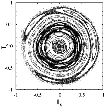
Figure 1: The map (23) with $d=100$ km revealing coherent ray clusters surviving in a model underwater waveguide under a noisy-like internal-wave perturbation (22) with a single vertical mode (28). The polar action-angle variables $I_{x}=(I/I_{s})\cos\theta$ and $I_{y}=(I/I_{s})\sin\theta$ are in units of the separatrix action $I_{s}$.

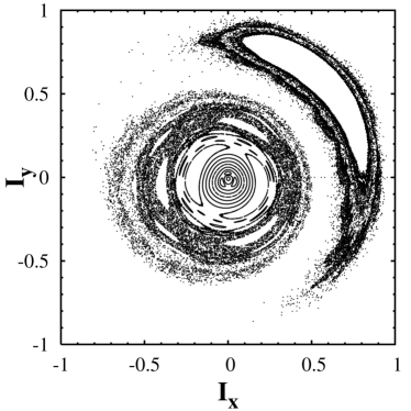
Figure 2: The same as in Fig. 1 but with five vertical modes (29), $d=100$ km.

Let the vertical oscillations contain a single mode only

$$X(z)=X_{1}\sin{\pi\chi(z)},$$ (28)

and the other parameters are as follows: $\varepsilon=0.0025$, $V(z)=(2z/B)e^{-2z/B}$, and $B=1$ km. We start with a large number of initial values of the ray action-angle variables in different regions of the phase space $(I_{0},\theta_{0})$ and compute their values at the distance $d=100$ km from a sound source with the respective equations of ray motion with a chosen realization of the noisy-like horizontal internal-wave perturbation (21) and the single vertical mode (28). Then we compute the ray variables with the same realization of noise at the same distance $d=100$ km, find $(I_{1},\theta_{1})$, and so on. The result of computing of the Poincaré map in the coordinates $I_{x}=(I/I_{s})\cos\vartheta$ and $I_{y}=(I/I_{s})\sin\vartheta$ with $I_{s}=I(H=-1)$, being the separatrix value of the action, is shown in Fig. 1. The map reveals numerous island-like regions of stability in the phase space corresponding to the resonance condition $mD(I)\simeq ld$, where $D(I)$ is a cycle length of a ray with a given action $I$. It should be noted that the outer chain with four islands corresponds to the same 1:1 resonance. Under a multi-frequency excitation, the system, being captured into the resonance $mD=ld$, is, simultaneously, in all the resonances $jmD=jld$, where $j$ is an integer.

Figure 3: The same as in Fig. 2 but with $d=500$ km.

Let us consider now a more complicated model with five vertical modes of internal waves

$$X(z)=\sum_{n=1}^{5}X_{n}\sin(n\pi\chi(z)+\phi_{n}),$$ (29)

where $X_{n}\propto n^{-2}$, and $\phi_{n}$ are random phases. The respective map (23) is shown in Fig. 2 with $d=100$ km. It follows from comparing Figs. 1 and 2 that complication in the vertical perturbation effects, mainly, the most steep rays corresponding to the outer resonance islands. The most outer island in Fig. 2 is separated from the other domains of stability by a layer of escaping rays (by escaping rays we mean the rays quiting by different reasons the sound waveguide during their propagation). With increasing $d$, the area of islands decreases but distinct islands of stability remain visible in the phase space at a rather long distance $d=500$ km (Fig. 3) even with five vertical modes of internal waves to be included in the model.

The practical question is: in which way the coherent ray clusters could be observed in real field experiments? What is measured in the field experiments is time arrivals of sound signals and the depths of their arrivals at a given range $R$ with the help of a vertical receiving array of hydrophones D92 ; W99 ; JASA . We compute the so-called timefront at $R=1000$ km solving not the map (23) but the equations of motion (16) with the stochastic perturbation (24) and (29). The prominent strips in Fig. 4 belong, mainly, to coherent ray clusters which survive even at the distance of 1000 km. It should be emphasized that similar strips have been found in the field experiments D92 ; W99 ; JASA .

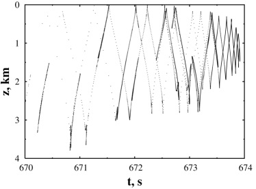
Figure 4: Timefront at the range $1000$ km under the stochastic perturbation (24) and (29): ray depth $z$ vs ray travel time t. Strips indicate coherent ray clusters.

Figure 5: Ray travel time $t$ vs starting momentum $p_{0}$ at the range $1000$ km. Shelves indicate coherent ray clusters.

In conclusion of this section we show manifestations of coherent ray clusters in the so-called $t-p_{0}$ plot. Fig. 5 demonstrates the ray travel time $t$ as a function of the starting ray momentum $p_{0}$ at the distance $R=1000$ km from a sound source for the model with purely horizontal random perturbation, i. e. Eq.(22) with $X(z)=1$. The main feature of this dependence is “shelves”, i. e. more or less flat segments in the $t-p_{0}$ plot. Each “shelf” corresponds to a coherent cluster. The “shelves” are distributed chaotically over the range of the starting momenta, and their positions depend on a specific realization of the random perturbation. Such “shelves” have been found with different kinds and realizations of the internal-wave induced random perturbation proving that appearing of coherent clusters is a common feature in the sound-waveguide propagation through a fluctuating ocean.

IV Clustering of passive particles in a two-dimensional flow

In this section we consider clustering in a simple two-dimensional flow of an ideal fluid with the dimensionless streamfunction

$${\Psi=\ln\sqrt{x^{2}+y^{2}}+\mu x+\varepsilon x~{}\xi(\tau)},$$ (30)

whose simplified version with $\xi(\tau)$ being a harmonic function has been introduced in Ref. BP01 to model advection of passive particles in a flow with a fixed point vortex (the first term in (30)), a stationary current along the axis $y$ with the normalized velocity $\mu$ (the second term), and a harmonically alternating current with the normalized velocity $\varepsilon$. In physical oceanography the streamfunction (30) is a simple kinematic model of mixing and transport in the flow around a topographical eddy over a seamount in the ocean randomly perturbed by wind in the surface layer or by small-scale turbulence. It is well known that the Hamiltonian equations of motion for particles (tracers) with Cartesian coordinates $x$ and $y$ in an incompressible two-dimensional flow are written as

$${\dot{x}=-\frac{\partial\Psi}{\partial y}=-\frac{y}{x^{2}+y^{2}}},$$ (31)

$${\dot{y}=\frac{\partial\Psi}{\partial x}=\frac{x}{x^{2}+y^{2}}+\mu+\varepsilon~{}\xi(\tau)}.$$

Figure 6: The map (6) with $T_{0}=6\pi$ revealing clusters of advected particles in a random velocity field with the amplitude $\varepsilon=0.01$ and the frequency band $\omega\in[2:5]$. The unperturbed frequency of rotation of particles around the point vortex $\omega_{0}$ and the polar angle $\varphi/\pi$ are in arbitrary units.

Figure 7: The averaged (over $T_{0}$) energy of particles $\left<E\right>$ vs their unperturbed frequency $\omega_{0}$: (a) $T_{0}=6\pi$ and (b) $T_{0}=30\pi$. Shelves indicate clusters of particles. Parameters of noise are given in caption to Fig. 6.

The configuration space of advection particles is the phase space of dynamical system (30), and it is possible to see noisy-induced clusters of particles in the flow (30) by a naked eye. We model the noise as a random function $\xi(\tau)$ consisting of a large number of harmonics

$${F(\tau)=\frac{1}{\sqrt{N+1}}\sum\limits_{n=0}^{N}\sin(\omega_{n}\tau+\varphi_{n})},$$ (32)

with random phases $\varphi_{n}$ and the frequencies

$${\omega_{n}=\omega_{b}+n\frac{\omega_{e}-\omega_{b}}{N}},\qquad\displaystyle{n=0,1,\dots,N},$$ (33)

distributed equally in the range $[\omega_{b}:\omega_{e}]$ between the lowest $(\omega_{b})$ and highest $(\omega_{e})$ frequencies. It is possible, in principle, to model the spectrum of an arbitrary form with the help of the series (32) introducing an amplitude factor depending on the frequency. Accordingly to the central limit theorem, $\xi(\tau)$ has a Gaussian distribution with zero expectation value because it is a large number of independent random variables. The factor $1/\sqrt{N+1}$ provides the variance to be equal to $1/2$.

Advection of passive particles under a single-mode perturbation without any noise has been considered it detail in Refs.PD04 ; JETP04 as a scattering problem: particles enter a mixing zone around the vortex with the incoming current and escape from it with an outcoming flow. The scattering has been shown to be chaotic in the sense that there is a nonattracting invariant set, consisting of unstable periodic, aperiodic, and marginally unstable orbits, that determines scattering and trapping of particles from the incoming flow. The scattering has been shown to be fractal in the sense that scattering functions (namely, the dependence of the trapping time for particles and of the number of times they wind around the vortex on the initial particle’s coordinates) are singular on a Cantor-like set of initial positions.

Now we are interested in what happens if that deterministic flow is perturbed by a weak noise. It should be noted, first of all, that fractality in the scattering functions does not disappear under noisy excitation, but the respective fractals have been shown to have more complicated hierarchical structure B05 ; U05 . In order to find noisy-induced clusters of particles we use the effective Poincaré map of the type of (6) with different values of the time interval $T_{0}$, the amplitude of noise $\varepsilon$, and the frequency range of noise $[\omega_{b}:\omega_{e}]$.

In Fig. 6a we demonstrate the clusters of the map of the type (6) with $T_{0}=6\pi$ in the plane of the frequency $\omega_{0}$ of rotation of particles around the vortex in the unperturbed system with $\varepsilon=0$ and the polar angle with $\tan\varphi=y/x$. A large number of particles advected by the flow (30) with $\mu=0.5$ and a chosen realization of the weak noise with the amplitude $\varepsilon=0.01$ and the medium-frequency range $\omega\in[2:5]$ has been chosen for simulation.

Indirect manifestations of clusters are seen in Fig. 7a as shelf-like segments in the dependence of the averaged (over $T_{0}$) energy of tracers $\left<E\right>$ on their unperturbed frequency $\omega_{0}$ at initial positions. With increasing the interval of mapping $T_{0}$, noisy-induced clusters reduce, of course, in their size, but even with $T_{0}=30\pi$, which is larger than the average period of perturbation almost by two orders of magnitude, the prominent shelves corresponding to small-size clusters are still seen in Fig. 7b.

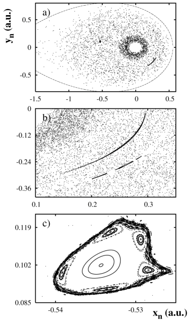
Figure 8: The map (6) with $T_{0}=2.3\pi$ revealing clusters of particles in a random velocity field with the amplitude $\varepsilon=0.1$ and the frequency band $\omega\in[9:10]$. (a) general view in the phase plane $(x,y)$, (b) and (c) magnifications of the respective clusters in (a). The dotted line is an unperturbed separatrix.

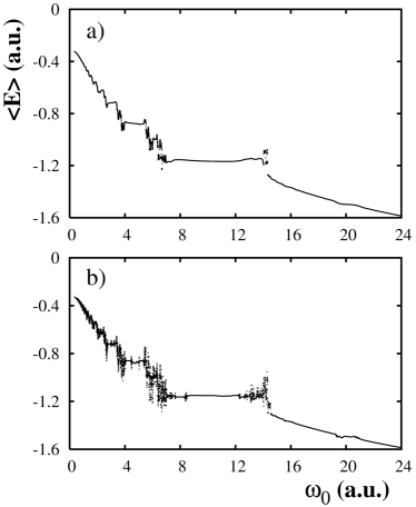
Figure 9: The averaged (over $T_{0}$) energy $\left<E\right>$ of particles vs their unperturbed frequency $\omega_{0}$: (a) $T_{0}=2.3\pi$ and (b) $T_{0}=10\pi$. Shelves indicate clusters of particles. Parameters of noise are given in caption to Fig. 8.

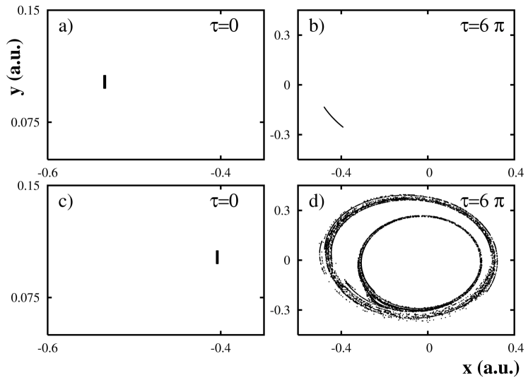
Figure 10: The compact evolution of a coherent cluster of particles (the upper panel) and deformation of an unstable patch of particles (the lower panel) in a random velocity field. Parameters of noise are given in caption to Fig. 8.

In order to test the effectiveness of the map of the type (6) in “catching” the noisy-induced clusters, we have carried out a series of numerical experiments with $\mu=0.5$ and the noise of the moderate amplitude $\varepsilon=0.1$ and the high-frequency range $\omega\in[9:10]$. Fig. 8a demonstrates the result of mapping with $T_{0}=2.3\pi$ on the configuration plane $(x,y)$, and Figs. 8b and c are magnifications of the respective clusters in Fig. 8a. Prominent chains of the islands of stability can survive under a rather strong noisy perturbation for a comparatively long time. Fig. 9 demonstrates shelf-like manifestations of noisy-induced clusters with $T_{0}=2.3\pi$ and $T_{0}=10\pi$.

To give a more direct manifestation of coherent clustering in a random flow that could be observed in real laboratory experiments with dye, we compare the evolution of patches of particles chosen in the regions of stability and instability in the configuration space. In the upper panel of Fig. 10 we show the evolution of a coherent cluster corresponding to the small black point (the region of stability for a given realization of noise) with coordinates $x\simeq-0.55$ and $y\simeq 0.1$ in Fig. 8a. More or less compact evolution of this patch with $10^{4}$ particles goes on up to, at least, $\tau=6\pi$. For comparison, the lower panel of Fig. 10 demonstrates on the same time interval the evolution of the patch with the same number of particles chosen initially close to the coherent cluster at $\tau=0$. The respective initial patch is deformed strongly at $\tau=6\pi$.

Clustering in the ocean is a common feature that can be seen, for example, in satellite images of the ocean surface. In resent years new observational tools — quasi-Lagrangian current following floats and drifters — have been used to observe velocity field in the ocean at different levels of depth (for a review see D91 ). In connection with our numerical observation of coherent clusters of passive particles in the simple kinematic ocean model, we would like to pay attention to the results of the SOFAR floats program in the POLYMODE experiment in the North Atlantic RPW86 . Up to forty neutrally buoyant floats at $700$ m and $1300$ m were used to provide a quasi-Lagrangian description of the structure and evolution of the mesoscale eddy field. Those floats can be considered as quasi-passive tracers in a weak noise environment. A large number of the deep floats revealed remarkably coherent motion over a two-month period.

V Conclusion

We proposed and justified a rather general method to find regions of stability in the phase space of oscillatory-like Hamiltonian systems driven by a weak noise with an arbitrary spectrum. Physical manifestations of these regions of stability, the so-called coherent clusters, have been demonstrated with two models in ocean physics. We have found coherent ray clusters in the model of underwater-waveguide sound proparagition through a randomly-fluctuating ocean and coherent clusters of passive particles in the two-dimensional flow modelling kinematically advection around a topographic eddy in the ocean.

In conclusion we would like to add two remarks about the properties of the effective Poincaré map (6). Firstly, the duration of the temporal interval $T_{0}$ in constructing the map can be chosen arbitrarily. Thus, if $\xi(t)$ is a stationary random process, the regions of stability in the phase space exist at any time moment. Secondly, the map (6) enables to prove definitely the existence of some regions of stability but not all of them. Really, the map, constructed with any given value of $T_{0}$, can reveal only those stable sets which correspond to the phase oscillations nearby the fixed points of the map. However, there exist another regions of stability looking as chaotic ones on the map. The topology of the map changes with varying the mapping time $T_{0}$, and some regions in the phase space, which look as pseudochaotic on the map at $T_{0}=T_{1}$, become stable at $T_{0}=T_{2}>T_{1}$. The total area of the regions of stability, survived under a weak noise at $t=T_{0}$, can be estimated as an area of superposition of all the stable sets detected by the map (6) with the mapping step varying from $T_{0}$ to $T_{c}$.

References

- (1) G.M. Zaslavsky, Hamiltonian Chaos and Fractional Dynamics (Oxford University Press, Oxford, 2004).
- (2) D.V. Makarov, M.Yu. Uleysky, and S.V. Prants, Chaos. 14, 79 (2004).
- (3) A.J. Lichtenberg and M.A. Lieberman, Regular and Stochastic Motion (Springer, New York, 1983).
- (4) V.I. Arnold, V.V. Kozlov, and A.I. Neishtadt, Mathematical Aspects of Classical and Celestial Mechanics. Encyclopaedia of Mathematical Sciences, vol.3. (Springer-Verlag, Berlin, 1988).
- (5) B.V. Chirikov, Phys. Rep. 52, 265 (1979).
- (6) A.B. Rechester, M.N. Rosenbluth, and R.B. White, Phys. Rev. A 23, 2664 (1981).
- (7) L.M. Brekhovskikh and Yu. Lysanov, Fundamentals of Ocean Acoustics (Springer-Verlag, Berlin, 1991).
- (8) Special issue of the J. Acoust. Soc. Am. 117(3), Pt.2 (2005).
- (9) L.D. Landau and E.M. Lifshitz, Mechanics (Nauka, Moscow, 1973; Pergamon Press, Oxford, 1976).
- (10) S.S. Abdullaev and G.M. Zaslavsky, Zh. Eksp. Teor. Fiz. 80, 524 (1981) [Sov. Phys. JETP 53, 265 (1981)].
- (11) S.S. Abdullaev and G.M. Zaslavsky, Usp. Fiz. Nauk 161, 1 (1991) [Sov. Phys. Usp. 34, 645 (1991)].
- (12) J. Simmen, S.M. Flatté, and Guang-Yu Wang, J. Acoust. Soc. Am. 102, 239 (1997).
- (13) M.G. Brown, J.A. Colosi, S. Tomsovic, A.L. Virovlyansky, M.A. Wolfson, and G.M. Zaslavsky, J. Acoust. Soc. Am. 113, 2533 (2003).
- (14) M.A. Wolfson and S. Tomsovic, J. Acoust. Soc. Am. 109, 2693 (2001).
- (15) T.F. Duda, S.M. Flatté, J.A. Colosi, B.D. Cornuelle, J.A. Hildebrand, W.S. Hodgkiss, P.F. Worcester, B.M. Howe, J.A. Mercer, and R.C. Spindel, J. Acoust. Soc. Am. 92, 939 (1992).
- (16) P.F. Worcester, B.D. Cornuelle, M.A. Dzieciuch, W.H. Munk, B.M. Howe, J.A. Mercer, R.C. Spindel, J.A. Colosi, K. Metzger, T.J. Birdsall, and A.B. Baggeroer, J. Acoust. Soc. Am. 105, 3185 (1999).
- (17) D.V. Makarov, M.Yu. Uleysky, and S.V. Prants, Pis’ma Z. Tekh. Fiz. 29 70 (2003) [Tech. Phys. Lett. 29, 430 (2003)].
- (18) D.V. Makarov, Thesis, Pacific Oceanological Institute, Vladivostok, 2004 (www.dynalab.poi.dvo.ru).
- (19) M.Yu. Uleysky, Thesis, Pacific Oceanological Institute, Vladivostok, 2005 (www.dynalab.poi.dvo.ru).
- (20) M.V. Budyansky, and S.V. Prants, Pis’ma Z. Tekh. Fiz. 27 51 (2001) [Tech. Phys. Letters. 27, 508 (2001)].
- (21) M. Budyansky, M. Uleysky, and S. Prants, Physica D 195, 369 (2004).
- (22) M.V. Budyansky, M.Yu. Uleysky, and S.V. Prants, Zh. Eksp. Teor. Fiz. 126, 1167 (2004) [JETP 99, 1018 (2004)].
- (23) M.V. Budyansky, Thesis, Pacific Oceanological Institute, Vladivostok, 2005 (www.dynalab.poi.dvo.ru).
- (24) R.E. Davis, Annu. Rev. Fluid Mech. 23, 43 (1991).
- (25) T. Rossby, J. Price, and D. Webb, J. Phys. Oceanogr. 16, 428 (1986).