Abstract

Integrable equations exhibit interesting conformal properties and can be written in terms of the so-called conformal invariants. The most basic and important example is the KdV equation and the corresponding Schwarz-KdV equation. Other examples, including the Camassa-Holm equation and the associated Camassa-Holm equation are investigated in this paper. It is shown that the Bäcklund transform is related to the conformal properties of these equations. Some particular solutions of the Associated Camassa-Holm Equation are discussed also.

PACS: 05.45.Yv, 02.30.Ik

Key Words: Schwarz Derivative, Conformal Invariants, Lax Pair, Integrable Systems, Solitons, Positons, Negatons.

1 Introduction

Integrable equations exhibit many extraordinary properties like infinitely many conservation laws, multi- Hamiltonian structures, soliton solutions etc. Many integrable equations in 1+1 dimensions like KdV, MKdV, Harry-Dym, Boussinesq equations possess interesting conformal properties as well [1, 2, 3, 4, 5]. They can be written in terms of the so-called independent conformal invariants of the function $\phi=\phi(x,t)$:

$$p_{1} = \frac{\phi_{t}}{\phi_{x}}$$

$$p_{2} = \{\phi;x\}\equiv\frac{\phi_{xxx}}{\phi_{x}}-\frac{3}{2}\frac{\phi_{xx}^{2}}{\phi_{x}^{2}}$$

Here $\{\phi;x\}$ denotes the Schwarz derivative. A quantity is called conformally invariant if it is invariant under the Möbius transformation

$$\phi \rightarrow \frac{\alpha\phi+\beta}{\gamma\phi+\delta},\qquad\alpha\delta\neq\beta\gamma.$$ (2)

For example, the KdV equation

$$u_{t}+au_{xxx}+3uu_{x}=0$$ (3)

($a$ is a constant) can be written in a Schwarzian form, i.e. in terms of the conformal invariants (1) as $p_{1}+ap_{2}=0$ or

$$\frac{\phi_{t}}{\phi_{x}}+a\{\phi;x\}=0$$ (4)

where

$$u=a\{\phi;x\}.$$ (5)

The KdV and Camassa-Holm (CH) [6] equations arise also as equations of the geodesic flow for the $L^{2}$ and $H^{1}$ metrics correspondingly on the Bott-Virasoro group [7, 8, 9]. The conformal properties of these equations and their link to the Bott-Virasoro group originate from the Hamiltonian operator

$$D_{3}\equiv a\partial^{3}+\partial u(x)+u(x)\partial$$ (6)

where $\partial\equiv\partial/\partial x$. $D_{3}$ is also known as the third Bol operator [10] and is the conformally covariant version of the differential operator $\partial^{3}$, see also [11]. $D_{3}$ defines a Poisson bracket [1]

$$\{f,g\}=\frac{1}{2\pi i}\int\Big{(}(a\partial^{3}+\partial u(x)+u(x)\partial)\frac{\delta f}{\delta u}\Big{)}.\frac{\delta g}{\delta u}dx$$ (7)

and KdV, CH and many other equations [12] can be written in the form

$$u_{t}=\{u,H\}$$ (8)

for some Hamiltonian $H$. On the other hand, suppose for simplicity that $u$ is $2\pi$ periodic in $x$, i.e.

$$u(x)=\sum^{\infty}_{-\infty}L_{n}e^{inx}-\frac{a}{2}$$ (9)

then the Fourier coefficients $L_{n}$ close a classical Virasoro algebra with respect to the Poisson bracket (7):

$$\{L_{n},L_{m}\}=(n-m)L_{n+m}+a(n^{3}-n)\delta_{n+m,0}$$ (10)

Therefore, it is natural to expect that equations which can be written in the form (8) exibit interesting conformal properties, and this is the case indeed [5, 11, 13, 14, 15]. In what follows we will concentrate on the Camassa-Holm and the associated Camassa-Holm equation.

2 The Camassa-Holm equation in Schwarzian form

The Camassa-Holm equation [6, 16]

$$u_{t}-u_{xxt}+au_{xxx}+3uu_{x}-2u_{x}u_{xx}-uu_{xxx}=0,$$ (11)

describes the unidirectional propagation of shallow water waves over a flat bottom [6, 17]. CH is a completely integrable equation [18, 19, 20, 21], describing permanent and breaking waves [22, 23]. Its solitary waves are stable solitons [24, 25, 26, 27]. CH arises also as an equation of the geodesic flow for the $H^{1}$ metrics on the Bott-Virasoro group [7, 8, 9]. The equation (11) admits a Lax pair [6]

$$V_{xx} = \Big{(}\frac{1}{4}-\lambda(m+\frac{a}{2})\Big{)}V$$ (12)

$$V_{t} = -\Big{(}\frac{1}{2\lambda}+u-a\Big{)}V_{x}+\frac{u_{x}}{2}V$$ (13)

where

$$m=u-u_{xx}.$$ (14)

In order to find the Schwarz form for the CH equation we proceed as follows. Let $V_{1}$ and $V_{2}$ be two linearly independent solutions of the system (12), (13) and let us define

$$\phi=\frac{V_{2}}{V_{1}}$$ (15)

Then, from (13) it follows that

$$\frac{\phi_{t}}{\phi_{x}}=-u+\Big{(}a-\frac{1}{2\lambda}\Big{)}$$ (16)

According to the Theorem 10.1.1 from [28] due to (12) we also have

$$\{\phi;x\}=2\lambda m+a\lambda-\frac{1}{2}$$ (17)

From (14), (16) and (17) we obtain the Schwarz-Camassa-Holm (S-CH) equation:

$$(1-\partial^{2})\frac{\phi_{t}}{\phi_{x}}+\frac{1}{2\lambda}\{\phi;x\}=\frac{3}{2}a-\frac{3}{4\lambda}$$ (18)

Since $\lambda$ is an arbitrary constant, one can take $\lambda=1/2a$ (if $a\neq 0$) and then the S-CH equation (18) acquires the form $(1-\partial^{2})p_{1}+ap_{2}=0$ or

$$(1-\partial^{2})\frac{\phi_{t}}{\phi_{x}}+a\{\phi;x\}=0$$ (19)

Applying the hodograph transform

$$x\rightarrow\phi,\qquad t\rightarrow t,\qquad\phi\rightarrow x$$ (20)

to the S-CH (19) and using the transformation properties of the Schwarzian derivative [28]

$$\{\phi;x\}=-\phi_{x}^{2}\{x;\phi\}$$ (21)

we obtain the following integrable deformation of the Harry Dym equation for the variable $v=1/x_{\phi}$:

$$v_{t}+v^{2}[v(v\partial_{\phi}^{-1}(v^{-1})_{t})_{\phi}]_{\phi}=av^{3}v_{\phi\phi\phi}$$

The equations (11) and (19) with $u=-\frac{\phi_{t}}{\phi_{x}}$ are not equivalent – as a matter of fact (19) implies (11), cf. [3]. It is often convenient to think that the Lax operator belongs to some Lie algebra, and the corresponding Jost solution- to the corresponding group. Thus the relation between $u$ and $\phi$ (see (15)) resembles the relation between the Lie group and the corresponding Lie algebra, as pointed out in [3]. More precisely, the following proposition holds:

Proposition 1

Let $\phi$ be a solution of (18). Then $V_{1}=\phi^{-1/2}_{x}$ and $V_{2}=\phi\phi^{-1/2}_{x}$ are solutions of (12), (13) with $u=-\frac{\phi_{t}}{\phi_{x}}-(\frac{1}{2\lambda}-a)$

Proof : It follows easily by a direct computation.

Note that the Proposition 1 is consistent with (15). From Proposition 1 it follows

Proposition 2

The general solution of (12), (13) is

$$V=\frac{A\phi+B}{\sqrt{\phi_{x}}}$$ (22)

where $A$ and $B$ are two arbitrary constants, not simultaneously zero.

Note that the expression (22) is covariant with respect to the Möbius transformation (2), i.e. under (2), the expression (22) transforms into an expression of the same form but with constants

$$A\rightarrow A^{\prime}=\frac{\alpha A+\gamma B}{\sqrt{\alpha\delta-\beta\gamma}},\qquad B\rightarrow B^{\prime}=\frac{\beta A+\delta B}{\sqrt{\alpha\delta-\beta\gamma}}.$$ (23)

3 The associated Camassa-Holm equations and the Bäcklund Transform

An inverse scattering method, which can be applied directly to the spectral problem (12) is not developed completely yet. However, the solutions of the CH (in parametric form) can be obtained by an implicit change of variables, which maps (12) to the well known spectral problem of the KdV hierarchy. This change of variables leads to the so-called Associated Camassa-Holm equation (ACH) [29]

$$p_{t^{\prime}}=p^{2}f_{x^{\prime}},\qquad f=\frac{p}{4}(\log p)_{x^{\prime}t^{\prime}}-\frac{p^{2}}{2}.$$ (24)

Indeed, the ACH is related to the CH equation (11) through the following change of variables:

$$p=\sqrt{m+\frac{a}{2}},\qquad f=-\frac{u}{2}-\frac{a}{4}$$ (25)

$$dx^{\prime}=\frac{1}{2}pdx+(-\frac{u}{2}+\frac{a}{2})pdt,\qquad dt^{\prime}=dt.$$ (26)

In what follows we will omit the dash from the new variables $x^{\prime}$ and $t^{\prime}$ and we will write simply $x$ and $t$ instead.

The ACH equation (24) is related to the KdV hierarchy [30, 31] since it may be written in the form

$$U_{t}=-2p_{x},\qquad U=-\frac{1}{2}\Big{(}\frac{pp_{xx}-\frac{1}{2}p_{x}^{2}+2}{p^{2}}\Big{)}$$ (27)

and the Lax pair for (27) is

$$V_{xx}+\Big{(}U-\frac{1}{\lambda}\Big{)}V=0,$$ (28)

$$V_{t}=\lambda\Big{(}pV_{x}-\frac{1}{2}p_{x}V\Big{)}.$$ (29)

The second part of (27) is the Ermakov-Pinney equation for $p$ (for a known $U$) [31, 20, 27, 32]. In order to obtain the Schwarzian form of the ACH equation, we introduce again $\phi=V_{2}/V_{1}$ as in (15), where now $V_{1}$ and $V_{2}$ are two linearly independent solutions of the system (28), (29). Then, by analogous arguments, from (28) it follows

$$U=\frac{1}{2}\{\phi;x\}+\frac{1}{\lambda},$$ (30)

and from (29)

$$p=\frac{\phi_{t}}{\lambda\phi_{x}}.$$ (31)

Using the relation between $p$ and $U$ given in the first part of (27), (30) and (31) we obtain the Schwarz-ACH (S-ACH) equation $p_{2,t}+(4/\lambda)p_{1,x}=0$, or

$$\{\phi;x\}_{t}+\frac{4}{\lambda}\Big{(}\frac{\phi_{t}}{\phi_{x}}\Big{)}_{x}=0.$$ (32)

Now one can easily check by a direct computation the validity of the following

Proposition 3

Let $\phi$ be a solution of S-ACH (32). Then $V_{1}=\phi^{-1/2}_{x}$ and $V_{2}=\phi\phi^{-1/2}_{x}$ are solutions of (28), (29) with

$$p=\frac{\phi_{t}}{\lambda\phi_{x}}.$$ (33)

As a corollary we find that the general solution of (28), (29), expressed through the solution of (32) is

$$V=\frac{A\phi+B}{\sqrt{\phi_{x}}}$$ (34)

where $A$ and $B$ are two arbitrary constants, not simultaneously zero. As we know the expression (34) is covariant under the Möbius transformations (2).

Definition 1

A transformation, which connects the solution $u$ of one equation to the solution $\widetilde{u}$ of the same (or another) equation is called a Bäcklund Transform (BT).

Such type of transformations were first discovered in relation to the sine-Gordon equation by A. Bäcklund around 1883. Usually BT depends on an arbitrary parameter which is called Bäcklund parameter.

The Lax pair (28), (29) has the following important property [31, 33], namely the BT for the ACH :

Proposition 4

If $V$ is a solution of the Lax pair (28), (29) with potentials $U$ and $p$, then $V^{-1}$ is a solution of (28), (29) with potentials

$$\widetilde{U} = U+2(\log V)_{xx},$$ (35)

$$\widetilde{p} = p-(\log V)_{xt}.$$ (36)

From (34) and (36) it now follows that the BT for the solution (33) of the ACH equation can be expressed through the solution of the S-ACH equation as follows:

$$\widetilde{p}=\frac{\phi_{t}}{\lambda\phi_{x}}-\Big{(}\log\frac{A\phi+B}{\sqrt{\phi_{x}}}\Big{)}_{xt}.$$ (37)

Since the constants $A$, $B$ are not simultaneously zero, one can always factor out one of the two constants, i.e. (37) obviously depends only on the ratio of these two constants (which is the Bäcklund parameter in this case).

We conclude this section with the following remark for the KdV equation. It is not difficult to see through similar considerations, that the Bäcklund Transform for the solution (5) of the KdV equation (3) is

$$\widetilde{u}=a\{\phi;x\}+4a\Big{(}\log\frac{A\phi+B}{\sqrt{\phi_{x}}}\Big{)}_{xx},$$ (38)

where $\phi$ is the solution of the S-KdV equation (4). Then the choice $A=0$ in (38) corresponds to the ’exotic’ Bäcklund Transform found by Galas in [34] and mentioned in [35].

4 On the solutions of the ACH and S-ACH equations

The solutions of the ACH and S-ACH equations can be constructed, following the scheme for the construction of the solutions of the KdV hierarchy [31, 36, 37, 38, 39, 40].

Let $v_{1},v_{2},\ldots v_{n}$ be $n$ different solutions of the Lax pair (28), (29) with potentials $U$ and $p$, taken at $\lambda=\lambda_{1},\lambda_{2},\ldots\lambda_{n}$ respectively and let $V_{1}$ and $V_{2}$ be two linearly independent solutions for some value $\lambda$. Consider the Wronskian determinants

$$W = W(v_{1},v_{1;1},\ldots,v_{1;m_{1}},v_{2},v_{2;1},\ldots,v_{2;m_{2}},\ldots,v_{n},v_{n;1},\ldots,v_{n;m_{n}})$$

$$W_{k} = W(v_{1},v_{1;1},\ldots,v_{1;m_{1}},\ldots,v_{n},v_{n;1},\ldots,v_{n;m_{n}},V_{k}),\qquad k=1,2,$$

where $v_{i;l}\equiv\partial_{\lambda}^{l}v_{i}$, $m_{i}$ are arbitrary nonnegative integers and the Wronskian determinant of $N$ functions $\varphi_{1},\varphi_{2},\ldots\varphi_{N}$ is defined by

$$W(\varphi_{1},\varphi_{2},\ldots\varphi_{N})=\det A,\qquad A_{ij}=\frac{d^{i-1}\varphi_{j}}{dx^{i-1}},\qquad i,j=1,2,\ldots,N.$$ (40)

The following generalization of the Crum theorem is valid for the KdV hierarchy and in particular for the ACH equation [37]:

Proposition 5

$\widetilde{V_{k}}=W_{k}/W$, $k=1,2$ are two linearly independent solutions of the Lax pair (28), (29) with potentials

$$\widetilde{U} = U+2(\log W)_{xx},$$ (41)

$$\widetilde{p} = p-(\log W)_{xt}.$$ (42)

From Proposition 5 it follows immediately that

$$\widetilde{\phi}=\frac{\widetilde{V_{2}}}{\widetilde{V_{1}}}=\frac{W_{2}}{W_{1}},\qquad\phi=\frac{V_{2}}{V_{1}}$$ (43)

are the solutions of the S-ACH (32), which correspond to the potentials

$$\widetilde{p}=\frac{\widetilde{\phi_{t}}}{\lambda\widetilde{\phi_{x}}},\qquad p=\frac{\phi_{t}}{\lambda\phi_{x}}.$$ (44)

In addition to the solutions mentioned in [31] one may construct also the so-called negaton and positon solutions (which are singular) and mixed soliton-positon-negaton solutions. For a detailed discussion on the positon and negaton solutions of KdV we refer to [40].

Let us return to (28) with $p=h=\mathrm{const}$, i.e. $U=-1/h^{2}$. Then it has the form

$$V_{xx}+E(h,\lambda)V=0,\qquad E(h,\lambda)=-\Big{(}\frac{1}{h^{2}}+\frac{1}{\lambda}\Big{)}.$$ (45)

The type of the solutions of (45) clearly depends on the sign of the constant $E(h,\lambda)$. If $E<0$ the independent solutions of (45) and (29) are

$$v_{1}(\lambda) = \cosh\Big{(}\sqrt{\frac{1}{\lambda}+\frac{1}{h^{2}}}(x-h\lambda t+x_{1}(\lambda))\Big{)},$$ (46)

$$v_{2}(\lambda) = \sinh\Big{(}\sqrt{\frac{1}{\lambda}+\frac{1}{h^{2}}}(x-h\lambda t+x_{2}(\lambda))\Big{)},$$ (47)

where $x_{1,2}(\lambda)$ are arbitrary functions. The simplest choice for $W$ in (41), (42) is $W=v_{1}$ or $W=v_{2}$ (Wronskian of order one), which corresponds to the one-soliton solution. The case $W=W(v_{1}(\lambda_{1}),v_{2}(\lambda_{2}))$ corresponds to the two-soliton solution, i.e. this solution describes the interaction of two solitons. However, according to (LABEL:eq33) it is possible to merge two or more identical solitons, taking

$$W = W(v_{1},v_{1;1},\ldots,v_{1;m_{1}}),$$ (48)

or

$$W = W(v_{2},v_{2;1},\ldots,v_{2;m_{2}}).$$ (49)

In physical terms $E(h,\lambda)$ is the energy of the soliton. Since the energy of the solitons is negative, (48) is called negaton of type $C$ and order $m_{1}$, and (49) is called negaton of type $S$ and order $m_{2}$, cf. [40]. The analogous considerations resulting from the following solutions of (45),

$$v_{1}(\lambda) = \cos\Big{(}\sqrt{\frac{1}{\lambda}-\frac{1}{h^{2}}}(x-h\lambda t+x_{1}(\lambda))\Big{)},$$ (50)

$$v_{2}(\lambda) = \sin\Big{(}\sqrt{\frac{1}{\lambda}-\frac{1}{h^{2}}}(x-h\lambda t+x_{2}(\lambda))\Big{)}$$ (51)

($0<\lambda\leq h^{2}$), whose energy is positive, $E>0$ leads naturally to the definition of positon of type $C$ and order $m_{1}$ via (48) and (42), and positon of type $S$ and order $m_{2}$, (49) and (42); cf. [40].

Due to (LABEL:eq33) it is possible to construct solutions, which describe the interaction between solitons, positons and negatons. I.e. the interaction between $n$ positons (of orders $m_{1},m_{2},\ldots,m_{n}$) and $N$ solitons is given by the $n$-positon – $N$ soliton solution ${}_{n}p_{N}$ of the ACH (24) which can be constructed from (42) taking the following solutions of the Lax pair (28), (29):

$$v_{i}=\cos\Big{(}\sqrt{\frac{1}{\lambda_{i}}-\frac{1}{h^{2}}}(x-h\lambda_{i}t+y_{i}(\lambda_{i}))\Big{)},\qquad i=1,\ldots n$$ (52)

$$\eta_{j}=\exp\Big{(}\sqrt{\frac{1}{\lambda_{n+j}}+\frac{1}{h^{2}}}(x-h\lambda_{n+j}t+x_{j})\Big{)}+\qquad\qquad\qquad\qquad$$ (53)

$$c_{j}\exp\Big{(}-\sqrt{\frac{1}{\lambda_{n+j}}+\frac{1}{h^{2}}}(x-h\lambda_{n+j}t+x_{j})\Big{)},\qquad j=1,\ldots N,$$ (54)

where $y_{i}(\lambda)$ are arbitrary functions of $\lambda$, $c_{j}$, $x_{j}$ are arbitrary constants and $0<\lambda_{i}\leq h^{2}$ for $i=1,\ldots,n$. Then (cf. [39])

$${}_{n}p_{N}(x,t) =$$

$$h\!\!\!\! - \!\!\!\!\Big{(}\log W(v_{1},v_{1;1},\ldots,v_{1;m_{1}},\ldots,v_{n},v_{n;1},\ldots,v_{n;m_{n}},\eta_{1},\ldots,\eta_{N})\Big{)}_{xt}.$$

As an example, we provide the one-positon solution of order one for the ACH, see also Fig. 1:

$${}_{1}p_{0}(x,t)=h-\frac{8h(h^{2}-\lambda_{1})\Big{(}\lambda_{1}+\lambda_{1}\cos z(x,t)+r(x,t)\sin z(x,t)\Big{)}}{\Big{(}2r(x,t)+h^{2}\sin z(x,t)\Big{)}^{2}}$$ (56)

where $\omega=\sqrt{\frac{1}{\lambda_{1}}-\frac{1}{h^{2}}}$, $y_{1}=a\lambda$, $a$ is an arbitrary constant;

$$z(x,t) = 2\omega(x-h\lambda_{1}t+a\lambda_{1}),$$

$$r(x,t) = \omega\Big{(}h^{2}x+\lambda_{1}(h^{2}-2\lambda_{1})(ht-a)\Big{)}.$$

5 Acknowledgements

The author is grateful to Prof. A. Constantin for helpful discussions and to the referees for valuable suggestions. The author also acknowledges funding from the Science Foundation Ireland, Grant 04/BR6/M0042.

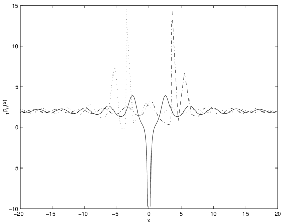
Figure 1: One-positon solution of the ACH equation, $a=0$, $h=2$, $\lambda_{1}=1$: $t=0$ – solid line; $t=-4$ – dashed line; $t=4$ – dotted line.

References

• [1] L. Dickey, Soliton Equations and Hamiltonian Systems, World Scientific, New Jersey, 2003.
• [2] I. Ya. Dorfman, Phys. Lett. A 125 (1987) 240.
• [3] G. Wilson, Phys. Lett. A 132 (1988) 445.
• [4] D. A. Depireux and J. Schiff, Lett. Math. Phys. 33 (1995) 99.
• [5] S.-y. Lou, X. Tang, Q.-P. Liu and T. Fukuyama, Z. Naturforsch. 57a (2002) 737.
• [6] R. Camassa, D. Holm, Phys. Rev. Lett. 71 (1993) 1661.
• [7] G. Misiolek, J. Geom. Phys. 24 (1998) 203.
• [8] A. Constantin and B. Kolev, Comment. Math. Helv. 78 (2003) 787.
• [9] A. Constantin, T. Kappeler, B. Kolev and P. Topalov, On geodesic exponential maps of the Virasoro group, Preprint No 13-2004, Institute of Mathematics, University of Zurich, (2004).
• [10] G. Bol, Abh. Math. Sem. Hamburger. Univ. Bd.16, Heft 3 (1949) 1.
• [11] F. Gieres, Int. J. Mod. Phys. A 8 (1993) 1.
• [12] A.S. Fokas, P.J. Olver, P. Rosenau, A plethora of integrable bi-Hamiltonian equations, in: Algebraic Aspects of Integrable Systems: In Memory of Irene Dorfman, A.S. Fokas and I.M. Gel’fand, eds., Progress in Nonlinear Differential Equations, vol. 26, Birkhauser, Boston, 1996, pp. 93-101.
• [13] J. Weiss, J. Math. Phys. 24 (1983) 1405.
• [14] J. Weiss, M. Tabor and G. Carnevale, J. Math. Phys. 24 (1983) 522.
• [15] M. C. Nucci, J. Phys. A: Math. Gen. 22 (1989) 2897.
• [16] A. Fokas, B. Fuchssteiner, Physica D 4 (1981) 821.
• [17] R.S. Johnson, J. Fluid. Mech. 457 (2002) 63.
• [18] R. Beals, D. Sattinger, J. Szmigielski, Adv. Math. 140 (1998) 190.
• [19] A. Constantin, H.P. McKean, Commun. Pure Appl. Math. 52 (1999) 949.
• [20] A. Constantin, Proc. R. Soc. Lond. A 457 (2001) 953.
• [21] J. Lenells, J. Nonlin. Math. Phys. 9 (2002) 389.
• [22] A. Constantin, J. Escher, Acta Mathematica 181 (1998) 229.
• [23] A. Constantin, Ann. Inst. Fourier (Grenoble) 50 (2000) 321.
• [24] R. Beals, D. Sattinger, J. Szmigielski, Inv. Problems 15 (1999) 1.
• [25] A. Constantin and W. Strauss, Commun. Pure Appl. Math. 53 (2000) 603.
• [26] A. Constantin and W. Strauss, J. Nonlin. Sci. 12 (2002) 415.
• [27] R. S. Johnson, Proc. R. Soc. Lond. A 459 (2003) 1687.
• [28] E. Hille, Ordinary Differential Equations in the Complex Domain, John Wiley, New York, 1976.
• [29] J. Schiff, Physica D 121 (1998) 24.
• [30] M. Fisher and J. Shiff, Phys. Lett. A 259 (1999) 371.
• [31] A. N. W. Hone, J. Phys. A: Math. Gen. 32 (1999) L307.
• [32] A. Shabat, J. Nonlin. Math. Phys. 12 (2005) 614.
• [33] A. N. W. Hone, V. B. Kuznetsov and O. Ragnisco, J. Phys. A: Math. Gen. 32 (1999) L299.
• [34] F. Galas, J. Phys. A: Math. Gen. 25 (1992) L981.
• [35] J. Schiff, preprint solv-int/9606004 (1996).
• [36] V. Matveev and M. Salle, Darboux Transformations and Solitons, Springer-Verlag, Berlin-Heidelberg, 1991.
• [37] V. Matveev, Phys. Lett. A 166 (1992) 205; erratum, ibid 168 (1993) 463.
• [38] V. Matveev, Phys. Lett. A 166 (1992) 209.
• [39] V. Matveev, J. Math. Phys. 35 (1994) 2955.
• [40] C. Rasinariu, U. Sukhatme and A. Khare, J. Phys. A: Math. Gen. 29 (1996) 1803.
Refer to caption