Abstract

In this paper, we presented a model of pulse-coupled oscillators distributed on a bidirectional ring with propagation delay. In numerical simulations based on this model, we observed phenomena of asynchrony in a certain range of delay factor $\alpha$. To find the cause of these phenomena, we used a new probability based approach of analyzing. In this approach, the mathematical expectation of influence on one oscillator’s phase change caused by its neighbor, which is regarded as a random factor, is calculated. By adding this expectation of influence into the firing map $h(\phi)$ introduced by Mirolla and Strogatz, a probability firing map $\mathbbm{H}$ is invented. By observing the behavior of $\mathbbm{H}$ ’s iteration from $\mathbbm{H}$ ’s graph, we successfully constructed a connection between the asynchrony phenomena and $\mathbbm{H}$ ’s graph.

keywords: oscillator, synchronization, pulse-couple, delay, bidirectional, ring, probability

I. Introduction &  Review

The phenomena of mutual synchronization widely exist in nature. For example, the synchronization of flashes of fireflies; the unison in which crickets and cicadae chirp; the pacemaker of the heart; and the synchronization of women’s menstrual period who live together.

A lot of researches have been done on this topic since last century. Mirolla and Strogatz[1] has studied a model of oscillators’ mutual synchronization with all-to-all connection and no delay pulse propagation. In their model, they introduced a phase-state function $f:[0,1]\to[0,1]$, which is required to be smooth, monotonic increasing, and concave down. With this $f$, the phase change of an oscillator receiving firing was described as $\phi^{t^{+}}=f^{-1}(f(\phi^{t^{-}}+\epsilon))$, where $\epsilon$ is the coupling strength. In their article, the initial conditions in wh ich the oscillators function will not achieve synchrony, was proved to be of Lebesgue measure zero, given the oscillators’ phase-state function satisfies the condition mentioned before.

Later, the dynamics synchronization under a threshold restriction $\phi_{c}$ was analyzed by Chia-Chu Chen [2]. With threshold included, the phase of an oscillator will not be “pulled up” by others’ firing when its phase $\phi\leqslant\phi_{c}$. Chen concluded that with $\phi_{c}<\frac{1}{2}$, synchronization can occur for almost all initial conditions.

In Mathar and Mattfeldt’s paper[3], the same conclusion was drawn on a collection of oscillators in all-to-all connections, but the differentiable constraint on the phase-state function introduced in[1] was removed. Instead $f$ was only required to be strictly concave and increasing. They proved the conclusion on two oscillators’ case by analyzing the iteration of the firing map $h(\phi)=f^{-1}(f(1-\phi)+\epsilon)$ and its fixed points. The conclusion was expanded the cases of a clique of $N$ oscillators by utilizing Fubini’s law. In the second part of the article, a propagation delay $\alpha$ was added into the model. A similar conclusion that oscillators with all the initial states except a Lebesgue measure zero set will achieve synchrony was reached on the model with delay.

Similar to this paper, a case of $N$ oscillators located on a unidirectional ring was discussed in [4]. In their model an oscillators pulled up to firing phase will fire, while in Mirolla & Strogatz’s model[1] it won’t. As a result of this mechanism, an “avalanche” effect exists (a chain of oscillators firing one immediately after another), and so helps the synchronization of the ring.

Díaz-Guilera, Pérez and Arenas[5] described the FD (firing + driving) process in the form of a vector’s multiplying a transformation matrix $\mathbb{M}$. Thus, the evolution of states of oscillators was evaluated by multiplying a series of matrices on the phase vector $(\phi_{1},\phi_{2},\dots\phi_{N})^{T}$. By comparing $\mathbb{M}$’s eigenvalues with $1$, the expected evolution result of the oscillators was classified into converging (repeller fixed points) and phase-locking (attractor fixed points). Also the properties of fixed points was related with sign of $\epsilon$. Similar methods were used in [6], which analyzed pattern formation on a ring of oscillators with couple strength $\epsilon<0$ (denoted as $\rho$ in this paper)selection.

In this paper, we first presented the model of oscillators distributed on a bidirectional ring with propagation delay. Based on this model, numerical simulation were made. From the results of the simulation, we spotted phenomena of asynchrony happening in a certain rang of propagation delaying factor $\alpha$ (see Fig 7). In purpose of explaining the asynchrony phenomena, we divided the analysis into three parts:

Step 1

For a pair of neighboring oscillators A and B, once they achieve $\alpha$-synchrony, their synchronization is easy to restore regardless of the influence from other neighbors. (Theorem 1)

Step 2

For a neighborhood consisted of oscillators B,C,D on the ring, we treat D as a random factor which uniformly distributed in $[0,1)$, thus we replace D with its mathematical expectation of influence on C.

Step 3

In a four-element neighborhood (A, B, C, D), if A and B have achieved $\alpha$-synchrony once, then we ignore A’s effect on B using the conclusion established in step 1. Also we substitute D with its mathematical expectation of influence on C calculated in step 2. After dealing with A and D, we are able to trace the synchronization process between B and C (See Formula 8).

By studying the iteration behavior of the firing map, which describes phase change of B and C, we successfully made a connection between the asynchrony phenomena (Fig 7) and the graph of the firing map (Fig 10).

II. The Model

In this paper we will discuss a system of $N$ oscillators distributed on a ring. This system includes the following properties:

Phase

For each oscillator $i$, there is a real number $\phi_{i}\in[0,1]$, called a phase variable, belongs to it to depict its phase.

Driving

As time goes by, the phase $\phi_{i}$ of each oscillator increases spontaneously at a constant speed $\displaystyle{\frac{\,\mathrm{d}\phi_{i}}{\,\mathrm{d}t}}=S=\frac{1}{T}$, here $T$ is the cycle period. For convenience we let $S=1$, by which we will also have $T=1$. See [1].

Firing

When an oscillator $i$’s phase $\phi_{i}$ reaches $1$, it will fire a pulse to other oscillators immediately. ([1])

Ring Topology

The firing of an oscillator will be received only by those oscillators that have connection to the firing one. In the bidirectional ring topology of this model, $i$’s pulse is received by $j$ only if $j\equiv i-1\ \mbox{or}\ i+1\,(\mbox{mod}N)$. See Fig 3.

Delay

Similar to [3], a factor of reaction and propagation delay is included in this model: an oscillator fired upon will not react to the pulse until a time delay $\alpha$ passes, (i.e. $i$ fires at $t_{0}$, $j$ only reacts at $t_{0}+\alpha$).

Period of no responding

The oscillator will not react if its phase is in the interval $[0,2\alpha)$ i.e. $j$ will not react if $\phi_{j}\in[0,2\alpha)$ at $t_{0}+\alpha$.

Coupling

When an oscillator $j$ reacts to a pulse (with precondition, $\phi_{j}^{t^{-}}\notin[0,2\alpha)\mbox{ at }t$ as the pulse is fired at $t-\alpha$), its phase is “pulled forward” for $\rho\cdot\phi_{j}^{t^{+}}+\epsilon$. That is

$$\phi_{j}^{t^{+}}=\begin{cases}(1+\rho)\cdot\phi_{j}^{t^{-}}+\epsilon\quad\quad&\mbox{if }(1+\rho)\cdot\phi_{j}^{t^{-}}+\epsilon<1\\ 0&\mbox{if }(1+\rho)\cdot\phi_{j}^{t^{-}}+\epsilon\geqslant 1\end{cases}$$

Here $\rho$ denotes the coupling strength, and $\epsilon$ the coupling constant. In this model we always have $\rho>0,\epsilon>0$. Note that when an oscillator’s $\phi$ is “pulled” up by others to reach 1, it will still fire.

Phase difference

The phase difference between two oscillators $i$ and $j$ are defined as

$$\mathbbm{D}(\phi_{i},\phi_{j})=\begin{cases}|\phi_{i}-\phi_{j}|\quad\quad&\mbox{if }|\phi_{i}-\phi_{j}|\leqslant\frac{1}{2}\\ 1-|\phi_{i}-\phi_{j}|&\mbox{if }|\phi_{i}-\phi_{j}|>\frac{1}{2}\end{cases}$$

With this definition, the difference between $\phi_{i}=0.9$ and $\phi_{j}=0.1$ is $0.2$, not $0.8$.

$\alpha$-synchronization

When oscillators $i$ and $j$ satisfy $\mathbbm{D}(\phi_{i},\phi{j})\leqslant\alpha$, they are $\alpha$-synchronized, or in other words, achieved $\alpha$-synchronization. See [3]. In addition, in a system of oscillators distributed on a ring, this system achieves $\alpha$-synchronization when each pair of “neighbor” achieves  $\alpha$-synchronization: $\forall i$, if $j\equiv i-1\ \mbox{or}\ i+1\,(\mbox{mod }N)$ $\Longrightarrow$ $\mathbbm{D}(\phi_{i},\phi_{j})\leqslant\alpha$. A system that has achieved $\alpha$-synchronization is showed in Fig 3.

Respond only once

An oscillator responds to a pulse from the same “neighbor” only once in one firing cycle. e.g. If in some way $i$ “catches” up with $j$ and fires the second time before $j$’s firing, $j$ does not respond to $i$’s second pulse. So far no previous models has added this restriction.

III. Numerical simulation

Before presenting a theoretical analysis on the dynamics of the system, first we provide some results on the numerical simulation.

a. Process of synchronization

The first experiment tracks the process of synchronization. In purpose of inspecting the course of a system’s synchronizing, a demonstration program is written in MATLAB, which shows the dynamics of oscillators represented by cylinders. Fig 3, 3, LABEL:graph:cylinder3 and 3 display four snapshots in a synchronization procedure.

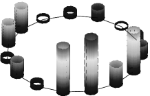
Figure 1: A ring of oscillators represented by cylinders. The height of cylinder depicts the phase of an oscillator. The connection lines on the bottom indicate the neighboring relationship.

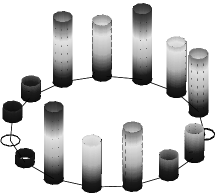
Figure 2: A system in its synchronization process.

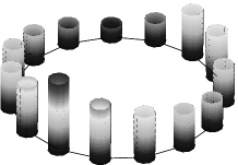
Figure 3: A system that achieved $\alpha$-synchronization

Also the count of $\alpha$-synchronized pairs ( $(\phi_{i},\phi_{i+1})$ s.t. $\mathbbm{D}(\phi_{i},\phi_{i+1})\leqslant\alpha$) is tracked in a numerical experiment. In Fig 4, the $x$ axis represents time, while $y$ axis represents the count of neighbors that are not $\alpha$-synchronized. From this figure we see that the trend of this system is achieving $\alpha$-synchrony.

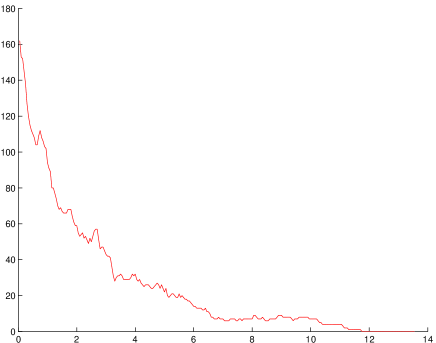
Figure 4: Count of pairs in asynchrony with the change of time. The system parameters are $\alpha=0.1$, $\rho=0.3$, $\epsilon=0.01$, $N=200$

In addition, a figure similar to [4] ’s grey level denotation is made. In Fig d.7, $x$ axis is the index of oscillators (that is to say, two pixels horizontally adjoining each other are neighboring oscillators $i$ and $i+1$), $y$ axis represents time (time increases via the direction of up-down), and the greylevel of a pixel $(i,t)$ on this figure depicts the phase $\phi_{i}$ of oscillator $i$ at time $t$ (the whiter, the nearer to 1, the blackest represents $\phi=0$). This figure is a vivid record of the whole synchronization process.

b. Testing time cost to achieve $\alpha$-synchronization

An experiment comparing the time used to achieve $\alpha$-synchronization with different system parameters is conducted. In the simulation, we tested systems with $N$ oscillators, and repeated the test for 100 times on 100 randomly generated samples, for each parameter combination. We generated 100 initial condition samples $\{S_{1},S_{2},\dots,S_{100}\}$, each $S_{k}=\{\phi_{0}^{(k)},\phi_{1}^{(k)},\dots,\phi_{N-1}^{(k)}\}$. For each combination of parameters such as $\alpha$, $\rho$, $\epsilon$, an average time used to achive $\alpha$-synchronization of the 100 samples is calculated. See algorithm (1) for a more strict description of the algorithm.

Algorithm 1 Calculating the time cost to achieve $\alpha$-synchronization with differnt $\rho$ and $\epsilon$

  Randomly generate 100 initial samples $\{S_{1},S_{2},\dots,S_{100}\}$.

  Generate the set of parameter values: $\widetilde{\rho}=\{\rho_{1},\rho_{2},\dots,\rho_{l}\}$, $\widetilde{\epsilon}=\{\epsilon_{1},\epsilon_{2},\dots,\epsilon_{m}\}$.

  for all $\rho\in\widetilde{\rho}$ do

     for all $\epsilon\in\widetilde{\epsilon}$ do

        $\text{timecost}\leftarrow 0$;

        for all $1\leqslant i\leqslant 100$ do

           timecost += (the time used to achieve $\alpha$-synchronization by $S_{i}$ under $\rho$, $\epsilon$)

        end for

        Draw a point $(\rho,\epsilon,\displaystyle\frac{\text{timecost}}{100})$on the $\rho-\epsilon-t$ graph.

     end for

  end for

A result is showed in Fig 5.

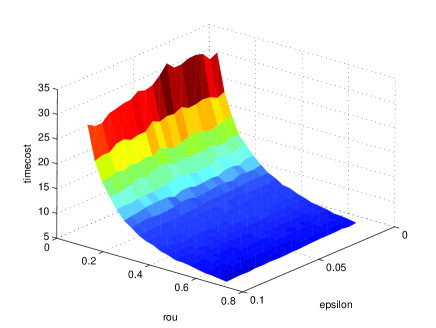
Figure 5: Average time cost to achieve $\alpha$-synchronization in 100 systems with different $\rho$ and $\epsilon$.

c. Phenomena of asynchrony

It is not always that, with any parameter, the system can eventually achieve $\alpha$-synchronization. Similar to algorithm 1, a program to count the configurations that fail to achieve $\alpha$-synchronization with a certain combination of parameters is designed. From Fig 7, it is easy to see that with $\alpha\in[0.01,0.1]$, asynchrony frequently happens.

For a clearer observation, a 2-D plot with respect to $\alpha-$count is drawn on Fig 7. Obviously, with $\alpha\approx 0.02$ and $\alpha\approx 0.05$, the chance of an asynchrony is large, while with $\alpha\geqslant 0.1$ the experiment always end in synchrony. In purpose of trying to find a reason to these phenomena, an analysis of the whole section IV. is implemented.

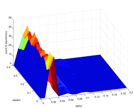
Figure 6: A $\alpha-\epsilon-$count graph that shows the count of configurations which don’t achieve synchrony before $t=100$. $\rho=0.3$, $N=200$, out of 100 samples.

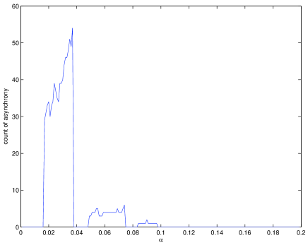
Figure 7: Count of initial configurations that fail to achieve $\alpha$-synchronization before $t=100$, out of 100 samples. $\rho=0.3$, $\epsilon=0.01$, $N=200$.

IV. Analysis of the Dynamics

In purpose of explaining phenomena observed in Fig 7, a step by step analysis is made in this section. First, we will review some useful notions introduced in previous works; then a new probability-based approach will be presented to find a cause of Fig 7.

a. Firing map

Similar to [3], first we check the dynamics of a system of two oscillators: A, B. Now Let a row vector $(\phi_{1},\phi_{2})$ to represent the state of two oscillators. Without loss of generality, we can always “shift” the phases of A, B into a form of $(\alpha,\phi)$, note that in this representation we change the order of components to make sure $\phi>\alpha$. After a FD process, the state of this pair becomes $(\alpha,\phi^{\prime})$ (a change of order from $(\phi^{\prime},\alpha)$). We define function $h:[0,1)\to[0,1)$ to describe the mapping $\phi\mapsto\phi^{\prime}$. Without considering the bounds, $h$ may simply be

$$h(\phi)=(1+\rho)\cdot(1+\alpha-\phi)+\epsilon$$ (1)

Now consider the restrictions on $h(\phi)$:

1. when $\phi\in[0,\alpha)$, there’s no definition on $h$ since we suppose $\phi\geqslant\alpha$. But for convenience we expand the domain of $h$ to $[0,1)$

2. when $\phi\in[\alpha,2\alpha)$, since they achieve $\alpha$-synchronization, there’s no effect on A from B’s firing.

3. when $\phi$ and $\alpha$ are “farther” away from $\alpha$, but still too “close”, B’s firing will pull A’s phase to reach $1$ and cause A’s immediate firing. We can calculate this bound $\delta_{\alpha}$:
   $h(\delta_{\alpha})=1\Longleftrightarrow(1+\rho)\cdot(1+\alpha-\delta_{\alpha})+\epsilon=1\Longleftrightarrow$

   $$\delta_{\alpha}=1+\alpha-\displaystyle{\frac{1-\epsilon}{1+\rho}}$$ (2)

Based on the discussion above, we define the firing map

$$h(\phi)=\begin{cases}2\alpha-\phi\quad&\mbox{if }0\leqslant\phi<2\alpha\\ 0&\mbox{if }2\alpha\leqslant\phi\leqslant\delta_{\alpha}\\ (1+\rho)\cdot(1+\alpha-\phi)+\epsilon&\mbox{if }\delta_{\alpha}<\phi<1\end{cases}$$ (3)

b. Jumping length

To inspect A’s “length” of phase that was “pulled” forward by B’s firing, we introduce the concept of Jumping Length. When A responds to B’s firing at time $t$, A’s jumping length is $\mathbbm{D}(\phi_{\text{A}}^{t^{+}},\phi_{\text{A}}^{t^{-}})$. Furthermore, on a standard two-oscillator configuration $(\alpha,\phi)$, the jumping length that A will have due to B’s firing is defined as

$$\mathcal{J}(\phi)=\begin{cases}0\quad&\mbox{if }\phi\in[0,2\alpha)\\ \phi-2\alpha&\mbox{if }\phi\in[2\alpha,\delta_{\alpha}]\\ \rho\cdot(1+\alpha-\phi)+\epsilon&\mbox{if }\phi\in(\delta_{\alpha},1)\end{cases}$$ (4)

And for a non-standard configuration $(\phi_{\text{A}},\phi_{\text{B}})$, where $(\phi_{\text{A}}<\phi_{\text{B}})$, the jumping length of A that will be caused by B: $\mathcal{J}^{\ast}\left(\phi_{\text{A}}\leftarrow\phi_{\text{B}}\right)$ is defined as

$$\mathcal{J}^{\ast}\left(\phi_{\text{A}}\leftarrow\phi_{\text{B}}\right)=\mathcal{J}\left(\phi_{\text{B}}-\phi_{\text{A}}+\alpha\right)$$ (5)

c. Stability of $\alpha$-synchronization

In a system of two oscillators, once the system achieves $\alpha$-synchronization, the synchrony will never be lost as the oscillators don’t respond to each other’s pulse all the time regarding to the rule delay in the model. But in the system of more than $2$ oscillators, each one is influenced by its two neighbors. Will a pair of oscillators that achieves $\alpha$-synchronization lose synchrony due to others’ coupling? Here we can show that if a pair is $\alpha$-synchronized once, they will restore their synchrony any time one of them reacts to the other one’s firing.

Theorem 1.

$\phi_{i}$ and $\phi_{i+1}$ ($\phi_{i})$ are neighboring oscillators that achieve $\alpha$-synchronization at one time:
$\exists t_{0}:\mathbbm{D}(\phi_{i}(t_{0}),\phi_{i+1}(t_{0}))\leqslant\alpha$. Then for any $t^{\ast}>t_{0}$ at which $i$ or $i+1$ fires, we will have
$\mathbbm{D}(\phi_{i}(t^{\ast}+\alpha),\phi_{i+1}(t^{\ast}+\alpha))\leqslant\alpha$ again.

Proof.

Without loss of generality, we suppose $\phi_{i+1}=\phi_{i}+d$, $0\leqslant d\leqslant\alpha$, and $k\in\{i,i+1\}$ the oscillator that will first fire (note that $i$ may “catch up” with $i+1$). Let $t^{\ast}$ be the time of $k$’s firing.

Case 1 — Neither $i$ or $i+1$ receives any pulse in [$t_{0}-\alpha,t^{\ast}$] :

Obviously without the influence of pulse outside the pair $i$ and $i+1$, these two oscillators will remain in synchrony:

$$\mathbbm{D}(\phi_{i}(t)),\phi_{i+1}(t))\leqslant\alpha,\forall t\in[t_{0},t^{\ast}+\alpha]$$

(See the figure on the right: the height of bars represents phase $\phi$, the two bars in the middle are $i$ and $i+1$. The leftmost and rightmost bars will not fire before $i+1$’s firing.)

Case 2 — $i+1$ receives a pulse and $i$ doesn’t receive one before $t^{\ast}$:

Suppose $i+2$ fires at $t_{1}$, then $i+1$ reacts to its pulse at $t_{2}=t_{1}+\alpha$

(i)$(1+\rho)\cdot\phi_{i+1}^{t_{2}^{-}}+\epsilon\geqslant 1$:

As the phase of $i+1$ reaches $1$, $i+1$ fires immediately and resets to 0 (by the way we have $t^{\ast}=t_{2}$)
After a time length of $\alpha$, $i$ reacts to the firing at $t_{3}=t^{\ast}+\alpha$.
$\because\phi_{i+1}=\phi_{i}+d$, $d\leqslant\alpha$,
$\therefore\phi_{i}^{t_{3}^{-}}=\phi_{i}^{t^{\ast}}+\alpha=\phi_{i+1}^{t^{\ast-}}-d+\alpha\geqslant\phi_{i+1}^{t^{\ast-}}$
$\Longrightarrow\phi_{i}^{t_{3}^{+}}=(1+\rho)\cdot\phi_{i}^{t_{3}^{-}}+\epsilon\geqslant(1+\rho)\cdot\phi_{i+1}^{t^{\ast-}}+\epsilon=(1+\rho)\cdot\phi_{i+1}^{t_{2}^{-}}+\epsilon\geqslant 1$
That is to say, $\phi_{i}$ is reset to $0$ at $t^{\ast}+\alpha$,
$\Longrightarrow\mathbbm{D}(\phi_{i},\phi_{i+1})=\mathbbm{D}(0,\alpha)=\alpha$,
which indicates $i$ and $i+1$ are $\alpha$-synchronized again.

(ii)$(1+\rho)\cdot\phi_{i+1}^{t_{2}^{-}}+\epsilon<1$:

After a time length $l=1+\alpha-\phi_{i+1}^{t_{2}^{+}}$, $i$ will respond to $i+1$’s firing.
Let $t_{3}=t^{\ast}+\alpha$ ( also $=t2+l$), then

$$(1+\rho)\cdot\phi_{i}^{t_{3}^{-}}+\epsilon = (1+\rho)\cdot(\phi_{i}^{t_{2}}+l)+\epsilon$$

$$= (1+\rho)\cdot(\phi_{i+1}^{t_{2}^{-}}-d+\alpha+1-\phi_{i+1}^{t_{2}^{+}})+\epsilon$$

$$> (1+\rho)\cdot(\phi_{i+1}^{t_{2}^{-}})+\epsilon+(1-\phi_{i+1}^{t_{2}^{+}})$$

$$= \phi_{i+1}^{t_{2}^{+}}+(1-\phi_{i+1}^{t_{2}^{+}})$$

$$= 1$$

Hence $\phi_{i}$ is reset to 0 at $t_{3}^{+}$, which implies $\mathbbm{D}(\phi_{i},\phi_{i+1})=\mathbbm{D}(0,\alpha)=\alpha$ after $i$ responds to the pulse from $i+1$
$\Longrightarrow$ the $\alpha$-synchronization remains.

So in case 2, the $\alpha$-synchronization will restore.

Case 3 — $i$ receives a fire before $t^{\ast}$

This case is divided into two sub-cases with respect to $k$ (whether $i$ “catches up” with $i+1$ or not).

(i) $k=i+1$

$i+1$ will be the first that fires and $i$ will reacts to its firing at $t_{3}=t^{\ast}+\alpha$
Imagine there is a “shadow” oscillator $\widetilde{i}$, which has a phase equal to $i$ at $t_{0}$: $\widetilde{\phi_{i}}^{t_{0}}=\phi_{i}^{t_{0}}$, but $\widetilde{i}$ doesn’t respond to $i-1$’s firing during $[t_{0},t^{\ast}+\alpha]$.
Then $\widetilde{i}$ ’s case is discussed in case 2.
$\Longrightarrow$ $\widetilde{\phi_{i}}^{t_{3}^{+}}\geqslant 1$.
And obviously we have $\widetilde{\phi_{i}}^{t_{3}^{-}}<\phi_{i}^{t_{3}^{-}}$
$\Longrightarrow$ $\phi_{i}^{t_{3}^{+}}\geqslant\widetilde{\phi_{i}}^{t_{3}^{+}}\geqslant 1$,
which is a proof a $i$ and $i+1$’s restoration of $\alpha$-synchronization.

(ii) $k=i$

If $i+1$ doesn’t receive a fire from $i+2$ before $t_{3}=t^{\ast}+\alpha$,
Similar to Case 2(ii), suppose $i-1$ fires at $t_{1}$, then $i$ reacts to its pulse at $t_{2}=t_{1}+\alpha$
After a time length $l=1+\alpha-\phi_{i}^{t_{2}^{+}}$, $i+1$ will respond to $i$’s firing.
No matter $i+1$ reacts to $i+2$ ’s pulse before $t^{\ast}$ or not, we have

$$(1+\rho)\cdot\phi_{i+1}^{t_{3}^{-}}+\epsilon \geqslant (1+\rho)\cdot(\phi_{i+1}^{t_{2}}+l)+\epsilon$$

$$\geqslant (1+\rho)\cdot(\phi_{i}^{t_{2}^{-}}+d+\alpha+1-\phi_{i}^{t_{2}^{+}})+\epsilon$$

$$> (1+\rho)\cdot(\phi_{i}^{t_{2}^{-}})+\epsilon+(1-\phi_{i}^{t_{2}^{+}})$$

$$= \phi_{i}^{t_{2}^{+}}+(1-\phi_{i}^{t_{2}^{+}})$$

$$= 1$$

That is $\mathbb{D}(\phi_{i}^{t_{3}},\phi_{i+1}^{t_{3}^{+}})=\mathbb{D}(\alpha,0)=\alpha$.

$\therefore$ the $\alpha$-synchronization remains if $i$ receives a fire before $t^{\ast}$, no matter $i+1$ receives or not.

So we have proven that an $\alpha$-synchronization will restore at the time when one of the once-synchronized oscillators reacts to its synchronized partner’s pulse. ∎

d. Estimation on Dynamics

The dynamics of a system on a bidirectional ring with delay is complex: each oscillator in it responds to both side of neighbors, while each neighbor is influenced by a farther neighbor. It’s not easy to trace the evolution of the system based on an exact event-tracing approach like in [1], or [4] as the order of firing will not change due to unidirectional connection and non-delay in their cases. So, in this model, we need to use a new probability based approach to study the dynamics of the system.

d.1 Neighborhood of three

Now consider a three-oscillators-composed neighborhood (B, C, D), in which B and C have not achieved $\alpha$-synchronization (because the purpose of this analysis is on the synchronization process of B and C). Let a standard configuration $(\alpha,\phi,\hat{\phi})$, ($\phi\geqslant 2\alpha$)be used to describe the starting state of this neighborhood at $t_{0}$. For a given $\hat{\phi}$, if $\hat{\phi}$ is in some certain area(which will be discussed in the next paragraph), C will have a coupling effect on B in current cycle. That is after a time of $(1+\alpha-\hat{\phi})$, $\phi$ is added up with $\mathcal{J}^{\ast}(\phi_{\leftarrow}\hat{\phi})$ — i.e. the state becomes $(\alpha+(1+\alpha-\hat{\phi}),\phi+(1+\alpha-\hat{\phi})+\mathcal{J}^{\ast}(\phi_{\leftarrow}\hat{\phi}),\alpha)$ at $t_{0}+(1+\alpha-\hat{\phi})$.

d.2 Domain of $\hat{\phi}$

For a given $\phi$, there is an interval $\mathcal{D}_{\phi}$ which $\hat{\phi}$ must be in, in order to affect $\phi$ in C’s current cycle. $\mathcal{D}_{\phi}$ is defined piecewise:

$$\mathcal{D}_{\phi}=\begin{cases}(\phi+\alpha,1)\cup[0,\alpha)\quad&\text{ if }\phi\in(2\alpha,1-\alpha)\\ (\alpha+\phi-1,\alpha)&\text{ if }\phi\in(1-\alpha,1)\end{cases}$$

To unite the definition, we extend $\hat{\phi}$ ’s domain from $[0,1)$ and treat $1+\hat{\phi}$ the same as $\hat{\phi}$. In this way $\mathcal{D}_{\phi}$ becomes

$$\mathcal{D}_{\phi}=(\phi+\alpha,1+\alpha)$$

d.3 Reducing three to two

With respect to D’s influence on C, there is no difference whether C’s “adding up” $\mathcal{J}^{\ast}(\phi_{\leftarrow}\hat{\phi})$ happens after a while or immediately. So, in purpose of analyzing the dynamics of (B, C) in one cycle, we can treat D’s coupling as if it happens immediately at $t_{0}$. That is, for this neighborhood $(\alpha,\phi,\hat{\phi})$, we can depict its state with one less opponent: $(\alpha,\phi+\mathcal{J}^{\ast}(\phi_{\leftarrow}\hat{\phi}))$ , by making D’s pulse into effect immediately and discard it from this neighborhood for its effect in this cycle is already done. So the representation of this neighborhood $(\alpha,\phi,\hat{\phi})$ becomes $(\alpha,\phi+\mathcal{J}^{\ast}(\phi_{\leftarrow}\hat{\phi}))$.

d.4 Random factor

By putting the neighborhood (B, C, D) back to the ring of oscillators, we may notice that B is also influenced by its left neighbor A, while D is affected by its right neighbor E. If we go on inspecting A and E, we have to face a very long chain of cause-and-effects. So, now we use a probability based approach to analyze the possible behavior of the system. That is, when analyzing the behavior of B and C, we consider A and D as random factors — their phases uniformly distribute on $[0,1)$.

d.5 Expectation of influence

For a standard configuration of B, C: $(\alpha,\phi)$, C is possible to be influenced by D’s firing before its reaching $0$. So we consider D’s phase $\hat{\phi}$ a random variable uniformly distributed on $[0,1)$. When $\hat{\phi}\in\mathcal{D}_{\phi}$, C will react to D’s firing before its own resetting. This response causes C’s phase to have a jumping forward of length $\mathcal{J}^{\ast}(\phi_{\leftarrow}\hat{\phi})$. So the mathematical expectation of C’s jumping length caused by random variable $\hat{\phi}$ is

$$E(\mathcal{J}^{\ast}(\phi_{\leftarrow}\hat{\phi}))$$ (7)

$$= P\{\hat{\phi}\in\mathcal{D}_{\phi}\}\cdot\frac{1}{\parallel\mathcal{D}_{\phi}\parallel}\int_{\mathcal{D}_{\phi}}\mathcal{J}^{\ast}(\phi_{\leftarrow}\hat{\phi})\,\mathrm{d}\hat{\phi}$$

$$= \frac{1-\phi}{1-\phi}\int_{\mathcal{D}_{\phi}}\mathcal{J}^{\ast}(\phi_{\leftarrow}\hat{\phi})\,\mathrm{d}\hat{\phi}$$

$$= \int_{\mathcal{D}_{\phi}}\mathcal{J}^{\ast}(\phi_{\leftarrow}\hat{\phi})\,\mathrm{d}\hat{\phi}$$

So in the neighborhood consisted by B, C, D ($\alpha,\phi,\hat{\phi}$), we regard D as a random factor and replace it by its “average” affection $E(\mathcal{J}^{\ast}(\phi_{\leftarrow}\hat{\phi}))$ on C. Thus we can analyze B,C’s dynamics in a cycle by inspecting $(\alpha,\phi+E(\mathcal{J}^{\ast}(\phi_{\leftarrow}\hat{\phi})))$. This replacement is demonstrated in Fig 8.

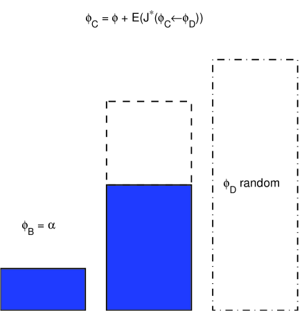
Figure 8: A demonstration of replacing $\phi_{\text{D}}$ with the mathematical expectation of influence that it may cause on C.

To calculate $\phi+E(\mathcal{J}^{\ast}(\phi_{\leftarrow}\hat{\phi}))$ using (7) and (5), we have

$$\phi+E(\mathcal{J}^{\ast}(\phi_{\leftarrow}\hat{\phi}))$$

$$= \phi+\int_{\mathcal{D}_{\phi}}\mathcal{J}^{\ast}(\phi_{\leftarrow}\hat{\phi})\,\mathrm{d}\hat{\phi}$$

$$= \phi+\int_{\phi+\alpha}^{1+\alpha}\mathcal{J}(\hat{\phi}-\phi+\alpha)\,\mathrm{d}\hat{\phi}$$

$$= \phi+\int_{2\alpha}^{1+2\alpha-\phi}\mathcal{J}(s)\,\mathrm{d}s$$

$$= \begin{cases}\phi+\displaystyle\int_{2\alpha}^{\delta_{\alpha}}(s-2\alpha)\,\mathrm{d}s+\displaystyle\int_{\delta_{\alpha}}^{1+2\alpha-\phi}(\rho\cdot(1+\alpha-s)+\epsilon)\,\mathrm{d}s\quad&\text{ if }1+2\alpha-\phi>\delta_{\alpha}\\ \phi+\displaystyle\int_{2\alpha}^{1+2\alpha-\phi}(s-2\alpha)\,\mathrm{d}s&\text{ if }1+2\alpha-\phi\leqslant\delta_{\alpha}\end{cases}$$

That is (see Fig 9 for a plot)

if $\phi<1+2\alpha-\delta_{\alpha}$:

$$\phi+E(\mathcal{J}^{\ast}(\phi_{\leftarrow}\hat{\phi}))=\phi+\frac{1}{2}\cdot(\delta_{\alpha}-2\alpha)^{2}+\frac{1}{2}\,(1+2\alpha-\delta_{\alpha}-\phi)[2\epsilon+(1-\delta_{\alpha}+\phi)\rho]$$

if $\phi\geqslant 1+2\alpha-\delta_{\alpha}$:

$$\phi+E(\mathcal{J}^{\ast}(\phi_{\leftarrow}\hat{\phi}))=\left(\frac{1+\phi}{2}\right)^{2}$$

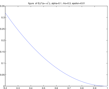
Figure 9: A plot of $E(\mathcal{J}^{\ast}(\phi\leftarrow\hat{\phi}))$

d.6 Absorption of $\alpha$-synchronized pairs

Suppose there is a pair of $\alpha$-synchronized oscillators A and B, whose states can be depicted in a standard form $(\phi_{0},\alpha)$ where $\phi_{0}=\alpha-d,0\leqslant d\leqslant\alpha$ (we can always make $\phi_{0}>\alpha$ with symmetry of the bidirectional ring). Oscillator C ($\phi_{1}$) is B’s right side neighbor. If $\mathbbm{D}(\phi_{\text{C}},\phi_{\text{B}})>\alpha$, we will find out that B and C are likely to achieve $\alpha$-synchrony, which looks like C is absorbed into an $\alpha$-synchronized pair near it.

Because A and B have already achieved $\alpha$-synchrony, according to Theorem 1, this pair will restore their $\alpha$-synchrony everytime they reacts to each other’s pulse. In this estimation, we ignore the small chance that A may catch up with B, so B only reacts to C’s pulse. Follow the mathematical expectation based approach, we may estimate B and C’s state as $(\alpha,\phi+E(\mathcal{J}^{\ast}(\phi_{\leftarrow}\hat{\phi})))$. After B’s reacting to C’s firing, the state becomes $(h(\phi+E(\mathcal{J}^{\ast}(\phi_{\leftarrow}\hat{\phi}))),\alpha)$. Adding an expectation of D’s influence on C again, the state goes to

$$(h(\phi+E(\mathcal{J}^{\ast}(\phi_{\leftarrow}\hat{\phi}))),\alpha+E(\mathcal{J}^{\ast}(\alpha_{\leftarrow}\hat{\phi})))$$

which is equivalent to

$$(h(\phi+E(\mathcal{J}^{\ast}(\phi_{\leftarrow}\hat{\phi})))-E(\mathcal{J}^{\ast}(\alpha_{\leftarrow}\hat{\phi})),\alpha)$$

in the next round it becomes

$$\Bigg{(}\alpha,h\bigg{(}h\left(\phi+E(\mathcal{J}^{\ast}(\phi_{\leftarrow}\hat{\phi}))\right)-E(\mathcal{J}^{\ast}(\alpha_{\leftarrow}\hat{\phi}))\bigg{)}\Bigg{)}$$

Note that $\mathcal{J}^{\ast}(\phi\leftarrow\hat{\phi})$ defined in (7) has a prerequisite of $\phi>2\alpha$, so we have to recalculate:

$$E(\mathcal{J}^{\ast}(\alpha\leftarrow\hat{\phi}))$$

$$= E(\mathcal{J}(\hat{\phi}))$$

$$= \int_{2\alpha}^{1}\mathcal{J}(s)\,\mathrm{d}s$$

$$= \int_{2\alpha}^{\delta_{\alpha}}(s-2\alpha)\,\mathrm{d}s+\int_{\delta_{\alpha}}^{1}\left(\rho\cdot(1+\alpha-s)+\epsilon\right)\,\mathrm{d}s$$

$$= \frac{1}{2}\,(\delta_{\alpha}-2\alpha)^{2}+(1-\delta_{\alpha})\left[\rho\,(1+\alpha)+\epsilon\right]-\frac{1}{2}\,(1-\delta_{\alpha})^{2}$$

We define the probability firing map:

$$\mathbbm{H}(\phi)=h\bigg{(}h\left(\phi+E(\mathcal{J}^{\ast}(\phi_{\leftarrow}\hat{\phi}))\right)-E(\mathcal{J}^{\ast}(\alpha_{\leftarrow}\hat{\phi}))\bigg{)}$$ (8)

Then similar to [1] and [3], the synchronization of B and C can be studied by analyzing the iteration of $\mathbbm{H}$. That is, whether C will be absorbed to an $\alpha$-synchronized pair (A,B) depends on whether $\exists k\in\mathbbm{N}$ s.t. $\mathbbm{H}^{(k)}(\phi)=0$, here $\mathbbm{H}^{(k)}$ is an iteration of $\mathbbm{H}$: $\mathbbm{H}^{(k)}=\mathbbm{H}(\mathbbm{H}^{(k-1)})$

d.7 Explanation of asynchrony phenomena with iteration of $\mathbbm{H}$

In purpose of analyzing the properties of $\mathbbm{H}$, its graphs are plotted with respect to different parameters. We noticed the change of the structure of $\mathbbm{H}$ ’s graph with different $\alpha$. Also, in the experiments mentioned in previous section, we observed that with $\alpha\geqslant 0.1$, systems often fail to achieve $\alpha$-synchronization. With the graphs of $\mathbbm{H}$ with different $\alpha$, such phenomenons are easier to explain. From Fig. 10, we can see that with $\alpha<0.1$, the $\mathbbm{H}$ ’s graph is primarily consistied of a skew part and two flat parts, defined as $N_{\mathbbm{H}}=\{x|\mathbbm{H}(x)=0\}$. Obviously, if $x\in N_{\mathbbm{H}}$, B and C will achieve synchrony in the next round. Even if $x\notin N_{\mathbbm{H}}$, as the slope of the skew part $[0,1]\backslash N_{\mathbbm{H}}$ is greater than 1, the value of $\mathbbm{H}^{k}(x)$ will eventually “fall” in to $N_{\mathbbm{H}}$, which results in $\mathbbm{H}^{k+1}(x)=0$.

As the value of $\alpha$ increases, the graph of $\mathbbm{H}(x)$ gradually becomes not so good looking. For $\alpha=0.02$ in Fig 10, we can find “pits” on the graph, which prohibits the iteration to reach $\mathbbm{H}^{k}(x)=0$. For example, the flat part $[0.1,0.15]$ will cause every initial values that in it to reach a fixed point $x^{\ast}\approx 0.11$, i.e. $\forall x\in[0,0.15]$, $\mathbbm{H}(x)=x^{\ast}$, where $\mathbbm{H}(x^{\ast})=x^{\ast}\neq 0$. This is an explanation of the happening of phenonemons of asynchrony in $\alpha=0.02$ observed in previous experiments in fig 7.

Also on the graph of $\alpha=0.05$, the same patterns are spotted: $\mathbbm{H}([0,0.15])\approx 0.1\in[0,0.15]$, which creates a fixed point of $\mathbbm{H}$ that attracts initial values in $[0,0.15]$.

However, with $\alpha=0.2$, the graph of $\mathbbm{H}$ in Fig (10) is in another pattern. A rough observation on this graph tells: for turning points $x_{1}\approx 0.25$, $x_{2}\approx 0.4$, $x_{3}\approx 0.75$, $x_{4}\approx 0.9$ of $y=\mathbbm{H}(x)$, $\mathbbm{H}([0,x_{1}])>x_{1}$, $\mathbbm{H}([x_{1},x_{2}])>x_{2}$, $\mathbbm{H}^{\prime}([x_{2},x_{3}])>1$ and $\mathbbm{H}([x_{3},x_{4}])=0$, $\mathbbm{H}([x_{4},1])\in[0,x_{1}]$, which means

$$\mathbbm{H} : [x_{4},1]\Rrightarrow[0,x_{1}]$$

$$\mathbbm{H} : [0,x_{1}]\Rrightarrow[x_{1},x_{2}]$$

$$\mathbbm{H} : [x_{1},x_{2}]\Rrightarrow[x_{2},x_{3}]$$

$$\mathbbm{H} : [x_{2},x_{3}]\Rrightarrow\Rrightarrow 0$$

So, for an arbitrary initial point $\phi_{0}\in[0,1]$, with iteration of $\phi_{k+1}=\mathbbm{H}(\phi_{k})$, we will inevitably have $\phi_{n}=0$ for some $n\in\mathbb{N}$.

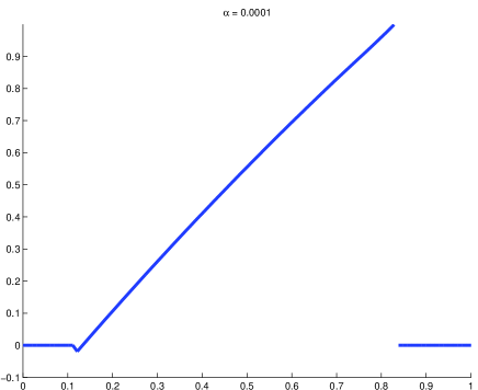
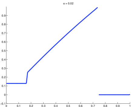
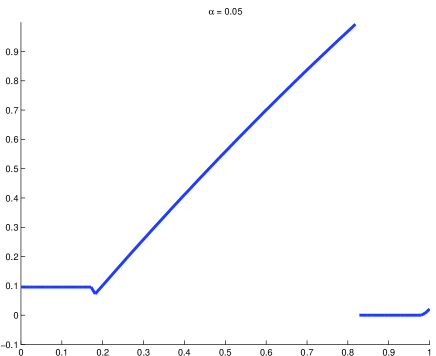
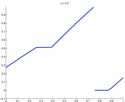
Figure 10: Graph of $\mathbbm{H}(\phi)$ with differnet $\alpha$, when $\rho=0.3$, $\epsilon=0.01$

V. Conclusions

In this paper we have proven that in each pair that once achieved $\alpha$-synchronization will restore their synchrony no matter how their neighbors acts. Then with comparison between the numerical simulation results and the properties of $\mathbbm{H}$, we have successfully established a cause-and-effect link between the synchronization behavior of the systems and their probability firing map $\mathbbm{H}$. With this application of $\mathbbm{H}$, it is reasonable to believe that the probability based approach presented in section (IV.) reaches the point of the problem.

VI. Further works

On Fig 5, a non-linear change of timecost with respect to $\alpha$ is clearly seen. But this phenomenon is not yet studied in this paper. Also, in section (IV.), we ignored a lot of affecting factors that may attribute to the result of the system’s evolution. And what is more, the reason of forming of patterns in $\mathbbm{H}$ should be searched with analytic studies on $E(\mathcal{J}^{\ast}(\phi\leftarrow\hat{\phi}))$ Besides, we would like to inspect synchronization phenomena when a central “host” oscillator is added, which has connection to all, or part of the oscillators on the circumference. We hope to work on those topics in further studies.

Acknowledgements

The author of this paper benefited a lot from Prof. Tianping Chen’s seminar, School of Mathematical Sciences, Fudan University.

Figure 11: This figure demonstrates an $\alpha$-synchronization process of 100 oscillators. $x$ axis represents the index of oscillators, $y$ axis represents time, grey level shows the phase of the oscillator (blackest: $\phi=0$, whitest: $\phi=1$). Inspired by [4].

References

- [1] Renato E. Mirolla and Steven H. Strogatz. Synchronization of pulse-coupled biological oscillators. SIAM. J. Appl. Math., 50:1645–1662, 1990.
- [2] Chia-Chu Chen. Threshold effects on synchronization of pulse-coupled oscillators. Physical Review E, 49:2668–2672, 1993.
- [3] Rdolf Mathar and Jürgen. Mattfeldt. Pulse-coupled decentral synchronization. SIAM. J. Appl. Math., 56:1094–1106, 1996.
- [4] José M.G. Vilar and Álvaro Corral. Synchronization of short-range pulse-coupled oscillators. arXiv:cond-mat/9807403, 1, 1998.
- [5] Albert Díaz-Guilera, Conrad J. Pérez, and Alex Arenas. Mechanisms of synchronization and pattern formation in a lattice of pulse-coupled oscillators. Physical Review E, 57:3820–3828, 1998.
- [6] X. Guardiola and A.Díaz-Guilera. Pattern selection in a lattice of pulse-coupled oscillators. Physical Review E, 60:3626–3632, 1999.
- [7] ALbert Díaz-Guilera and Conrad J. Perez-Vicente. Synchronization in a ring of pulsating oscillators with bidirectional couplings. arXiv:cond-mat/9812221, 1, 1998.
- [8] Vladimir N Belykh, Igor V Belykh, and Martin Hasler. Connection graph stability method for synchronized coupled chaotic systems. Physica D, 195:159–187, 2004.