Algebraic Closed Geodesics on a Triaxial Ellipsoid

Abstract

We propose a simple method of explicit description of families of closed geodesics on a triaxial ellipsoid $Q$ that are cut out by algebraic surfaces in ${\mathbb{R}}^{3}$. Such geodesics are either connected components of spatial elliptic curves or of rational curves.

Our approach is based on elements of the Weierstrass–Poncaré reduction theory for hyperelliptic tangential covers of elliptic curves, the addition law for elliptic functions, and the Moser–Trubowitz isomorphism between geodesics on a quadric and stationary solutions of the KdV equation. For the case of 3-fold and 4-fold coverings, explicit formulas for the cutting algebraic surfaces are provided and some properties of the corresponding geodesics are discussed.

1 Introduction

One of the best known classical integrable systems is the geodesic motion on a triaxial ellipsoid $Q\subset{\mathbb{R}}^{3}$. By introducing ellipsoidal coordinates on $Q$, the problem was reduced to hyperelliptic quadratures by Jacobi ([9]) and was integrated in terms of theta-functions of a genus 2 hyperelliptic curve $\Gamma$ by Weierstrass in [18].

A generic geodesic on $Q$ is known to be quasiperiodic and oscillate between 2 symmetric curvature lines (caustics).

It is of a certain interest to find conditions for a geodesic on $Q$ to be periodic (closed) and to describe such geodesics explicitly. At first sight this problem has a standard solution: by introducing action–angle variables $\{I_{1},I_{2},\phi_{1},\phi_{2}\}$ one can define frequencies

$$\dot{\phi}_{1}=\Omega_{1}(I_{1},I_{2}),\quad\dot{\phi}_{2}=\Omega_{2}(I_{1},I_{2}).$$

Then the geodesic is closed if and only if the rotation number $\Omega_{2}/\Omega_{1}$ is rational.

However, the frequencies $\Omega_{j}$ are known to be linear combinations of Abelian integrals on the hyperelliptic curve, hence the condition on the rotation number implies a transcendental equation on the constants of motion and the parameters of the problem. In practice, this appears to be useless for an exact description of closed geodesics.

Such a description can be made much more explicit when the hyperelliptic curve $\Gamma$ turns out to be a covering of an elliptic curve $\cal E$ and a certain holomorphic differential reduces to a holomorphic differential on $\cal E$. Then the corresponding geodesic itself is a spatial elliptic curve, which covers $\cal E$, or a rational curve and, as an algebraic subvariety in ${\mathbb{R}}^{3}$ (${\mathbb{C}}^{3}$), it can be represented as a connected component of the intersection of the ellipsoid $Q$ with an algebraic surface. In the sequel, such class of geodesics will be referred to as algebraic closed geodesics.

Conversely, one can also show that any algebraic closed geodesic on an ellipsoid must be a connected component of an elliptic or a rational curve.

Studying closed geodesics on quadrics is a classical problem. Surprisingly, we did not find any reference to its explicit solution in the classical or modern literature. Here we can only quote the paper [5], which studied the case of a 2-fold covering of an elliptic curve, when the solution is expressed in terms of two elliptic functions of time with different period lattices. Since the periods are generally incommensurable, the corresponding geodesics are not periodic but quasi-periodic.

Note that in the problem of periodic orbits of the Birkhoff billiard inside an ellipsoid much more progress has been made (see [6, 7, 14]).

Contents of the paper.

The paper proposes a simple approach to explicit description of algebraic surfaces $\cal V$ in ${\mathbb{R}}^{3}$ that cut out closed geodesics on $Q$. It is based on elements of the Weierstrass–Poncaré theory of reduction of Abelian functions (see, e.g.,[12, 3, 4]), addition law for elliptic functions, and the remarkable relation between geodesics on a quadric and stationary solutions of the KdV equation (the Moser–Trubowitz isomorphism) described in [11] and recently revisited in [1] in connection with periodic orbits of geodesic billiards on an ellipsoid.

Namely, for each genus 2 hyperelliptic tangential cover of an elliptic curve we construct a one-parameter family of plane algebraic curves (so called polhodes). Appropriate connected components of the polhodes have a form of Lissajou curves and describe closed geodesics in terms of the two ellipsoidal coordinates $\lambda_{1},\lambda_{2}$ on $Q$. The geodesics of one and the same family are tangent to the same caustic on $Q$ and the parameters of the ellipsoid are functions of the moduli of the elliptic curve.

Since equations of the polhodes depend only on the symmetric functions $\lambda_{1}+\lambda_{2}$, $\lambda_{1}\lambda_{2}$, they can be rewritten in terms of Cartesian coordinates in ${\mathbb{R}}^{3}$ thus giving the above mentioned algebraic surfaces $\cal V$.

Our family of closed geodesic contains special ones, which have mirror symmetry with respect to principal coordinate planes in ${\mathbb{R}}^{3}$. In particular, for the case of 3-fold and 4-fold coverings of an elliptic curve, the special geodesics are cut out by quadratic and, respectively, cubic surfaces in ${\mathbb{R}}^{3}$, as illustrated in Figures 5.4 and 6.3.

Depending on how to assign the parameters of the ellipsoid and of the caustic to the branch points of the hyperelliptic curve, one can obtain closed geodesics with or without self-intersections on $Q$.

2 Linearization of the geodesic flow on the
ellipsoid and some elliptic solutions

We first briefly recall the integration of the geodesic motion on an $n$-dimensional ellipsoid

$$Q=\left\{\frac{X_{1}^{2}}{a_{1}}+\cdots+\frac{X_{n+1}^{2}}{a_{n+1}}=1\right\}\subset{\mathbb{R}}^{n+1}=(X_{1},X_{2},\dots,X_{n+1}),$$

$$0<a_{1}<\cdots<a_{n}<a_{n+1}.$$

Let $t$ be the natural parameter of the geodesic and $\lambda_{1},\dots,\lambda_{n}$ be the ellipsoidal coordinates on $Q$ defined by the formulas

$$X_{i}^{2}=a_{i}\frac{(a_{i}-{\lambda}_{1})\cdots(a_{i}-{\lambda}_{n})}{\prod_{j\neq i}(a_{i}-a_{j})}\,,\qquad i=1,\dots,n+1.$$ (2.1)

In these coordinates and their derivatives $d\lambda_{k}/dt$ the total energy $\displaystyle\frac{1}{2}(\dot{X},\dot{X})$ takes a Stäckel form, and after time re-parameterization

$$dt=\lambda_{1}\cdots\lambda_{n}\,ds,$$ (2.2)

the evolution of $\lambda_{i}$ is described by quadratures

$$\frac{\lambda_{1}^{k-1}d\lambda_{1}}{2\sqrt{-R(\lambda_{1})}}+\cdots+\frac{\lambda_{n}^{k-1}d\lambda_{n}}{2\sqrt{-R(\lambda_{n})}}=\Bigg{\{}\begin{aligned} ds\quad\mbox{ for }&k=1\,,\\ 0\quad\mbox{ for }&k=2,\dots,n,\end{aligned}$$ (2.3)

$${R}(\lambda)=\lambda(\lambda-a_{1})\cdots(\lambda-a_{n+1})(\lambda-c_{1})\cdots(\lambda-c_{n}),$$

where $c_{k}$ are constants of motion.

This implies integrability of the system by the Liouville theorem. The generic invariant varieties of the flow are $n$-dimensional tori with a quasiperiodic motion. The corresponding geodesics are tangent to one and the same set of $n-1$ confocal quadrics $Q_{c_{1}},\dots,Q_{c_{n-1}}$ of the confocal family

$$Q_{c}=\left\{\frac{X_{1}^{2}}{a_{1}-c}+\cdots+\frac{X_{n+1}^{2}}{a_{n+1}-c}=1\right\}\subset{\mathbb{R}}^{n+1}.$$ (2.4)

In particular, generic geodesics on a 2-dimensional ellipsoid fill a ring bounded by caustics, the lines of intersection of $Q$ with confocal hyperboloid $Q_{c_{1}}$.

The quadratures (2.3) involve $n$ independent holomorphic differentials on the genus $n$ hyperelliptic curve $\Gamma=\{\mu^{2}=-R(\lambda)\}$,

$$\omega_{k}=\frac{\lambda^{k-1}d\lambda}{2\sqrt{{R}(\lambda)}}\,,\qquad k=1,\dots,n$$ (2.5)

and give rise to the Abel–Jacobi map of the $n$-th symmetric product $\Gamma^{(n)}$ to the Jacobian variety of $\Gamma$,

$$\int\limits^{P_{1}}_{P_{0}}\omega_{k}+\cdots+\int\limits^{P_{n}}_{P_{0}}\omega_{k}=u_{k},\qquad P_{k}=\left(\lambda_{k},\sqrt{-{R}(\lambda_{k})}\right)\in\Gamma,$$ (2.6)

where $u_{1},\dots,u_{n}$ are coordinates on the universal covering of Jac$(\Gamma)$ and $P_{0}$ is a fixed basepoint, which we choose to be the infinity point $\infty$ on $\Gamma$.

Since $u_{1}=s+$const and $u_{2},\dots,u_{n}=$const, the geodesic motion in the new parameterization is linearized on the Jacobian variety of $\Gamma$.

The inversion of the map (2.6) applied to formulas (2.1) leads to the following parameterization of a generic geodesic in terms of $n$-dimensional theta-functions $\theta(w_{1},\dots,w_{n})$ associated to the curve $\Gamma$,

$$X_{i}(s)=\varkappa_{i}\,\frac{\theta[\eta_{i}](w_{1},\dots,w_{n})}{\theta[\Delta](w_{1},\dots,w_{n})},\qquad i=1,\dots,n+1,$$ (2.7)

where $\Delta=(\delta^{\prime\prime},\delta^{\prime})$, $\eta_{i}=(\eta_{i}^{\prime\prime},\eta_{i}^{\prime})\in{\mathbb{R}}^{2n}/2{\mathbb{R}}^{2n}$ are certain half-integer theta-characteristics, the arguments $w_{1},\dots,w_{n}$ depend linearly on $u_{1},\dots,u_{n}$, and therefore on $s$, and $\varkappa_{i}$ are constant factors depending on the moduli of $\Gamma$ only.

For the classical Jacobi problem $(n=2)$, the complete theta-functional solution was presented in [18], and, for arbitrary dimensions, in [10], whereas a complete classification of real geodesics on $Q$ was made in [2].

Periodicity problem and a solution in terms of elliptic functions.

As mentioned in Introduction, we restrict ourselves with the case when a geodesic is periodic in the complex parameter $s$, namely, double-periodic. This implies that the solution (2.7) can be expressed in terms of elliptic functions of $s$.

As an example, following von Braunmuhl [5], consider the geodesic problem on 2-dimensional quadric ($n=2$) and suppose that the parameters $a_{i},c_{j}$ in (2.3) are such that the curve $\Gamma$ becomes birationally equivalent to the following canonical curve

$$w^{2}=-z(z-1)(z-\alpha)(z-\beta)(z-\alpha\beta),$$

$\alpha,\beta$ being arbitrary positive constant. Then, as widely described in the literature (see, e.g., [12, 3, 4]), $\Gamma$ covers two different elliptic curves

$$\ell_{\pm}=\{W_{\pm}^{2}=Z_{\pm}(1-Z_{\pm})(1-k_{\pm}Z_{\pm})\},\qquad k_{\pm}^{2}=-\frac{(\sqrt{\alpha}\mp\sqrt{\beta})^{2}}{(1-\alpha)(1-\beta)}$$

with covering relations

$$Z_{+}=Z_{-} =\frac{(1-\alpha)(1-\beta)z}{(z-\alpha)(z-\beta)},$$ (2.8)

$$W_{\pm} =-\sqrt{(1-\alpha)(1-\beta)}\,\frac{z\mp\sqrt{\alpha\beta}}{(z-\alpha)^{2}(z-\beta)^{2}}\,w.$$

Thus, $\Gamma$ is a 2-fold covering of $\ell_{-}$ and $\ell_{+}$.

Both holomorphic differentials $\omega_{1},\omega_{2}$ on $\Gamma$ reduce to linear combinations of the holomorphic differentials on $\ell_{+}$ and $\ell_{-}$, namely

$$\frac{dZ_{\pm}}{W_{\pm}}=\frac{z\mp\sqrt{\alpha\beta}}{w}\,dz.$$

Then a linear combination of equations (2.3) for $n=2$ yields

$$\int_{\infty}^{\lambda_{1}}\frac{z-\sqrt{\alpha\beta}}{w}\,dz+\int_{\infty}^{\lambda_{2}}\frac{z-\sqrt{\alpha\beta}}{w}\,dz =-s\sqrt{\alpha\beta}+\mbox{const}\,,$$

$$\int_{\infty}^{\lambda_{1}}\frac{z+\sqrt{\alpha\beta}}{w}\,dz+\int_{\infty}^{\lambda_{2}}\frac{z+\sqrt{\alpha\beta}}{w}\,dz =\;s\sqrt{\alpha\beta}+\mbox{const}\,.$$

Inversion of these quadratures lead to solutions for $X_{i}$ in terms of elliptic functions of the curves $\ell_{\pm}$, whose arguments both depend on the time parameter $s$. Then, since their periods are generally incommensurable, the corresponding geodesics remain to be quasi-periodic.

This observation shows that not any case of covering $\Gamma$ to an elliptic curve results in closed geodesics on $Q$. In the next section we consider other types of coverings and obtain sufficient condition for a geodesic to be an elliptic curve.

3 Hyperelliptic tangential covers and closed
geodesics on an $n$-dimensional ellipsoid

Consider a genus $n$ compact smooth hyperelliptic surface $G$, whose affine part $G_{A}\subset{\mathbb{C}}^{2}=(z,w)$ is given by equation

$$w^{2}=-R_{2n+1}(z),$$

$R_{2n+1}(z)$ being a polynomial of degree $2n+1$. The curve $G$ is obtained from $G_{A}$ by gluing the infinite point $\infty$. Let $\{\varOmega_{1}(P),\dots,\varOmega_{n}(P)\}$, $P=(z,w)\in G$ be a basis of independent holomorphic differentials on $G$. One can also write $\varOmega_{j}(P)=\phi_{j}(P)\,d\tau$, where $\tau$ is a local coordinate in a neibourhood of $P$. Next, let $\Lambda$ be the lattice in ${\mathbb{C}}^{n}$ generated by $2n$ independent period vectors $\oint(\varOmega_{1},\dots,\varOmega_{n})^{T}$.

The curve $G$ admits a canonical embedding into its Jacobian variety Jac$(G)={\mathbb{C}}^{n}(u_{1},\dots,u_{n})/\Lambda$,

$$P\mapsto{\cal A}(P)=\int_{\infty}^{P}(\varOmega_{1},\dots,\varOmega_{n})^{T},$$ (3.1)

so that $\infty$ is mapped into the neutral point (origin) in Jac$(G)$ and

$${\bf U}=\frac{d}{d\tau}{\cal A(P)}\bigg{|}_{P=\infty}=(\phi_{1}(\infty),\dots,\phi_{n}(\infty))^{T}$$

is the tangent vector of $G\subset$Jac$(G)$ at the origin.

Now assume that $G$ is an $N$-fold covering of an elliptic curve ${\cal E}$, which we represent in the canonical Weierstrass form

$${\cal E}=\left\{(\wp^{\prime}(u))^{2}=4\wp^{3}(u)-g_{2}\wp(u)-g_{3}\equiv 4(\wp-e_{1})(\wp-e_{2})(\wp-e_{3})\right\}.$$ (3.2)

Here $\wp(u)=\wp(u\mid\omega,\omega^{\prime})$ denotes the Weierstrass elliptic function with half-periods $\omega,\omega^{\prime}$ and $u\in{\mathbb{C}}/\{{\mathbb{Z}}\omega+{\mathbb{Z}}\omega^{\prime}\}$. The parameters $g_{2},g_{3}$ provide moduli of the curve.

Assume also that under the covering map $\pi\,:\,G\mapsto{\cal E}$ the infinite point $\infty\in G$ is mapped to $u=0$.

In the sequel we concentrate on hyperelliptic tangential coverings $\pi\,:\,G\mapsto{\cal E}$, when ${\cal E}$ admits the following canonical embedding onto Jac$(G)$

$$u\mapsto(u_{1},\dots,u_{n})=u{\bf U}.$$

That is, the images of ${\cal E}$ and $G$ in Jac$(G)$ are tangent at the origin . The motion of tangential covering was introduced in [16, 17] in connection with elliptic solutions of the KdV equation (see also [3, 4, 15]).

Namely, let $\theta(u_{1},\dots,u_{n})$ be the theta-function associated to the covering curve $G$ and $\Theta$ be the theta-divisor, codimension one subvariety of ${\rm Jac}(\Gamma)$ defined by equation $\theta[\Delta]({\bf u})=0$, where $[\Delta]$ is the special theta-characteristic in the solution (2.7).

Theorem 3.1.

([13]) For an arbitrary vector ${\bf W}\in{\mathbb{C}}^{g}$, the transcendental equation

$$\theta({\bf U}x+{\bf W})=0,\qquad x\in{\mathbb{C}},$$ (3.3)

has exactly $N$ solutions $x=q_{1}({\bf W}),\dots,x=q_{N}({\bf W})$ (possibly, with multiplicity).

That is, the complex flow on Jac$(G)$ in ${\bf U}$-direction intersects the theta-divisor $\Theta$ or any its translate at a finite number of points. This property is exceptional: for a generic hyperelliptic curve $G$ the number of such intersections is infinite.

Note that in the local coordinates $u_{1},\dots,u_{n}$ on Jac($G$) corresponding to the standard basis of holomorphic differentials

$${\bar{\omega}}_{k}=\frac{z^{k-1}\,dz}{w}\,,\qquad k=1,\dots,n,$$ (3.4)

one has ${\bf U}=(0,\dots,0,2)^{T}$.

According to the Poincaré reducibility theorem (see e.g., [3]), apart from the curve $\cal E$, the Jacobian of $G$ contains an $(n-1)$-dimensional Abelian subvariety ${\cal A}_{n-1}$. For $n=2$ the subvariety is just another elliptic curve covered by $G$.

Notice that for the case $n=2$, explicit algebraic expressions of the covers and coefficients of hyperelliptic curves are known for $N\leq 8$ (see [17]).

Double periodic geodesics on an ellipsoid.

The algebraic geometrical property described by Theorem 3.1 gives a tool for a description of double-periodic geodesic flow on the $n$-dimensional quadric $Q$, which is linearized on the Jacobian of the hyperelliptic curve $\Gamma$ in Section 2. Namely, let the genus $n$ curves $G$ and $\Gamma$ are related via birational transformation of the form

$$\lambda=\frac{\alpha}{(z-\beta)},\quad\mu=\frac{w}{(z-\beta)^{n+1}},$$ (3.5)

where $(\beta,0)$ is a finite Weierstrass point on $G$ and $\alpha$ is an arbitrary positive constant. Then the following theorem proved in [1] holds.

Theorem 3.2.

To any hyperelliptic tangential cover $G\mapsto{\cal E}$ such that all the Weierstrass points of $G$ are real, one can associate an $(n-1)$-parametric family of different closed real geodesics on an $n$-dimensional ellipsoid $Q$ that are tangent to the same set of confocal quadrics $Q_{c_{1}},\dots,Q_{c_{n-1}}$. The parameters of the ellipsoid ($a_{i}$) and of the quadrics ($c_{j}$) are related to branch points of $G$ via the transformation (3.5).

Remark.

It is natural to consider a closed geodesic as a curve on $Q$ and not as a periodic solution of the geodesic equations that depends on the initial point on the curve as on a parameter. That is, we disregard this parameter in the above family of closed real geodesics.

Proof of Theorem 3.2. The transformation (3.5) sends the points $\infty$ and $(\beta,0)$ on $G$ to the Weierstrass points ${\cal O}=(0,0)$ and, respectively, $\infty$ on $\Gamma$. Then, identifying the curves $G$ and $\Gamma$, as well as their Jacobians, we find that the ${\bf U}$-flow on Jac($G$), which is tangent to the canonically embedded hyperelliptic curve $\Gamma\subset\mbox{Jac}({\Gamma})$ at $\infty$, is represented as the flow on Jac($\Gamma$) which is tangent to the embedded $\Gamma\subset{\rm Jac}(\Gamma)$ at ${\cal O}$, and vice versa. In the coordinates on Jac$(\Gamma)$ corresponding to the basis (2.5), the latter flow has direction $(1,0,\dots,0)^{T}$ and thus coincides with the linearized geodesic flow on $Q$.

This remarkable relation was first described in [11] as the Moser–Trubowitz isomorphism between stationary $n$-gap solutions of the KdV equation and generic (quasiperiodic) geodesics on an $n$-dimensional quadric.

Next, let us fix a real constant $d$ and the confocal quadric $Q_{d}$ of the family (2.4) such that the geodesics with the constants of motion $c_{1},\dots,c_{n-1}$ have a non-empty intersection with $Q\cap Q_{d}$. In view of (2.1), when a geodesic $X(s)$ intersects $Q\cap Q_{d}$, one of the points $P_{i}=(\lambda_{i},\mu_{i})$ on the curve $\Gamma$ (without loss of generality we choose it to be $P_{n}$) coincides with one of the points $E_{d\pm}=(d,\pm\sqrt{R(d)})$. Under the Abel–Jacobi map (2.6) with $P_{0}=\infty$, the condition $P_{n}=E_{d\pm}$ defines two translates of the theta-divisor

$$\Theta_{d\pm}=\{\theta[\Delta]({\bf u}\mp q/2)=0\}\subset{\rm Jac}(\Gamma),\qquad q=\int_{E_{d-}}^{E_{d+}}(\varOmega_{1},\dots,\varOmega_{n})^{T}\in{\mathbb{C}}^{n}.$$

A geodesic is doubly-periodic if and only if it intersects $Q\cap Q_{d}$ at a finite number of complex points. In this case the linearized flow on ${\rm Jac}(\Gamma)$ must intersect $\Theta_{d\pm}$ at a finite set of points too. In view of the Moser–Trubowitz isomorphism and Theorem 3.1, this holds if $\Gamma$ is a hyperelliptic tangential cover of an elliptic curve ${\cal E}$. Then, under the transformation (3.5) with an appropriate $\beta$, the real Weierstrass points on $\Gamma$ give real and positive parameters $a_{i},c_{j}$ of the doubly-periodic geodesic.

Finally, there is an $(n-1)$-dimensional family of elliptic curves $\cal E$ in Jac($G$), which is locally parameterized by points of their intersection with the Abelian subvariety ${\cal A}_{n-1}$. This gives rise to an $(n-1)$-dimensional family of the doubly-periodic geodesics. $\boxed{}$

Remark.

Since for any chosen $N$-fold tangential cover $G\mapsto{\cal E}$ the branch points of $G$ are functions of the two moduli $g_{2},g_{3}$, the parameters $a_{i},c_{j}$ are uniquely determined by them and by the rescaling factor $\alpha$ in (3.5). This implies that not any ellipsoid $Q$ may have doubly-periodic geodesics associated with the given degree of covering as described by Theorem 3.2. One can show that even in the simplest case of a triaxial ellipsoid ($n=2$) and $N=3$ or 4, for any fixed positive $a_{1},a_{2}$ there exists only a finite number of possible $c,a_{3}$ for which the geodesics are doubly-periodic.

Naturally, this does not exclude the existence of such geodesics for other degrees of tangential coverings or those obtained from a periodic flow on Jac($G$) via a birational transformation different from (3.5), or even just closed geodesics, which are not doubly-periodic. However, the latter, if exist, cannot be algebraic curves in view of the following property.

Lemma 3.3.

Any algebraic closed geodesic on ellipsoid $Q\subset{\mathbb{R}}^{n}$ is a connected component of an elliptic or rational curve.

Proof. Let a closed geodesic be a connected component of an algebraic curve $\cal C$. Since the geodesic flow on $Q$ is linearized on an unramified covering of Jac$(\Gamma)$, $\cal C$ must be an unramified covering of an algebraic curve ${\cal C}_{0}\subset{\rm Jac}(\Gamma)$ and and, moreover, ${\cal C}_{0}$ must be a one-dimensional Abelian subvariety. Then, if $\Gamma$ is a regular curve and, therefore, Jac$(\Gamma)$ is compact, ${\cal C}_{0}$ can be only elliptic. If $\Gamma$ has singularities (when, for example, $c_{j}=a_{i}$ and the geodesic lies completely in hyperplane $X_{i}=0$) and its generalized Jacobian is not compact, then ${\cal C}_{0}$ can be also a rational curve. In both cases $\cal C$, as an unramified covering of ${\cal C}_{0}$, can be only elliptic or a reducible rational curve. $\boxed{}$

In the case $n=2$ the algebraic closed geodesics on a triaxial ellipsoid can explicitly be expressed in terms of symmetric functions of the two ellipsoidal coordinates $\lambda_{1},\lambda_{2}$ on $Q$. As a result, such geodesics can be rewritten in terms of Cartesian coordinates in ${\mathbb{R}}^{3}$. We shall describe this procedure in the next section.

4 Genus 2 hyperelliptic tangential covers, algebraic polhodes, and cutting algebraic surfaces in ${\mathbb{R}}^{3}$

Suppose that the genus 2 hyperelliptic curve $G$

$$w^{2}=-\prod_{k=1}^{5}(z-b_{k})$$ (4.1)

is an $N$-fold tangential covering of the elliptic curve ${\cal E}$ in (3.2). Then, according to the Poincaré reducibility theorem, $G$ is also an $N$-fold covering of another elliptic curve

$${\cal E}_{2}=\left\{W^{2}=-\left(4Z^{3}-G_{2}Z-G_{3}\right)\equiv-4(Z-E_{1})(Z-E_{2})(Z-E_{3})\right\},$$

the parameters $G_{2},G_{3}$ being functions of the moduli $g_{2},g_{3}$.

Let $U\in{\mathbb{C}}$ be uniformization parameter such that $Z=\tilde{\wp}(U)$, $W=\tilde{\wp}^{\prime}(U)$, and $\tilde{\wp}$ is the Weierstrass function associated to the curve ${\cal E}_{2}$. As above, assume that the point $\infty\in G$ is mapped to $U=0$. Then one can show that the map $\pi:\,G\rightarrow{\cal E}_{2}$ is described by formulas

$$Z={\cal Z}(z),\quad W=w^{k}\,{\cal W}(z),$$ (4.2)

where $k$ is a positive odd integer number and ${\cal Z}(z),{\cal W}(z)$ are rational functions of $z$ such that ${\cal Z}(\infty)=\infty$. The second relation in (4.2) implies that the Weierstrass points on $G$ are mapped to branch points on ${\cal E}_{2}$.

Consider the canonical embedding of $G$ to its Jacobian variety ${\mathbb{C}}^{2}=(u_{1},u_{2})/\Lambda$,

$$P=(z,w)\mapsto{\cal A}(z,w)=\left(\int_{\infty}^{P}\frac{dz}{w},\int_{\infty}^{P}\frac{z\,dz}{w}\right)^{T}.$$

The image of the embedding is the theta-divisor $\Theta$ that passes through the origin in Jac$(G)$ and is tangent to vector ${\bf U}=(0,1)^{T}$.

The second covering $\pi:\,G\rightarrow{\cal E}_{2}$ is lifted to the Jacobian variety of $G$. Namely, for any point ${\cal Q}\in{\cal E}_{2}$ and $\pi^{-1}({\cal Q})=\left\{P^{(1)},\dots,P^{(N)}\right\}\in G$, one has

$$\int\limits_{\infty}^{P^{(i)}}\frac{dz}{w}=\kappa\int\limits_{\infty}^{\cal Q}\frac{dZ}{W},$$ (4.3)

where $\kappa$ is a constant rational number depending on the degree $N$ only. This implies that $z$-coordinates of the $N$ points of intersection of a complex $u_{2}$-line ($u_{1}=$const) with $G=\Theta\subset\mbox{Jac}(G)$ are the roots of the first equation in (4.2) with $Z=Z({\cal Q})$ (see also [15]).

Now let $P_{1}=(z_{1},w_{1}),P_{2}=(z_{1},w_{2})\in G$ and consider the full Abel–Jacobi map

$${\cal A}(P_{1})+{\cal A}(P_{2})=(u_{1},u_{2})^{T}.$$ (4.4)

Assume that $u_{1},u_{2}$ evolve according to ${\bf U}$-flow, that is $u_{1}=$const. Hence $z_{1},z_{2}$ satisfy the equations

$$\dot{z}_{1}=\frac{w_{1}}{z_{1}-z_{2}},\quad\dot{z}_{2}=\frac{w_{1}}{z_{2}-z_{1}}.$$ (4.5)

This imposes a relation between coordinates of $P_{1}$ and $P_{2}$ on $G$. In the generic case, the relation is transcendental one and the coordinates are quasiperiodic functions of time. However, if $G$ is a tangential covering of an elliptic curve, then the relation becomes algebraic and can be found explicitly in each case of covering. Namely, let us set

$$U_{1}=\int\limits_{\infty}^{\pi(P_{1})}\frac{dZ}{W},\quad U_{2}=\int\limits_{\infty}^{\pi(P_{2})}\frac{dZ}{W},\quad\mbox{and}\quad U_{*}=U_{1}+U_{2}.$$ (4.6)

In view of (4.3) and the condition $u_{1}=$const, the first equation in (4.4) implies $U_{*}=$const.

Next, due to the addition theorem for elliptic functions,

$$\left|\begin{array}[]{ccc}1&\tilde{\wp}(U_{1})&\tilde{\wp}^{\prime}(U_{1})\\ 1&\tilde{\wp}(U_{2})&\tilde{\wp}^{\prime}(U_{2})\\ 1&\tilde{\wp}(-U_{*})&\tilde{\wp}^{\prime}(-U_{*})\end{array}\right|=0,$$ (4.7)

or, in the integral form

$$\tilde{\wp}(U_{*})+\tilde{\wp}(U_{1})+\tilde{\wp}(U_{2})=-\frac{1}{4}\left[\frac{\tilde{\wp}^{\prime}(U_{1})-\tilde{\wp}^{\prime}(U_{2})}{\tilde{\wp}(U_{1})-\tilde{\wp}(U_{2})}\right]^{2},$$

the coordinates $Z_{1}=\tilde{\wp}(U_{1}),Z_{2}=\tilde{\wp}(U_{2})$ are subject to the constraint

$$2G_{3}+G_{2}\left(Z_{1}+Z_{2}\right) +4\wp(U_{*})\left(Z_{2}-Z_{1}\right)^{2}-4Z_{2}Z_{1}\left(Z_{1}+Z_{2}\right)$$

$$\quad=-2\sqrt{4Z_{1}^{3}-G_{2}Z_{1}-G_{3}}\sqrt{4Z_{2}^{3}-G_{2}Z_{2}-G_{3}}.$$

Then, taking square of both sides, simplifying, factoring out $(Z_{1}-Z_{2})^{2}$, and replacing $Z_{1},Z_{2}$ by the expressions ${\cal Z}(z_{1}),{\cal Z}(z_{2})$ from (4.2), we arrive at generating equation

$$16 \left({\cal Z}(z_{2})-{\cal Z}(z_{1})\right)^{2}\widetilde{\wp}_{*}^{2}$$

$$+\left[16G_{3}+8G_{2}\left({\cal Z}(z_{1})+{\cal Z}(z_{2})\right)-32{\cal Z}(z_{1}){\cal Z}(z_{2})({\cal Z}(z_{1})+{\cal Z}(z_{2}))\right]\widetilde{\wp}_{*}$$

$$+16G_{3}\left({\cal Z}(z_{1})+{\cal Z}(z_{2})\right)+8G_{2}{\cal Z}(z_{1}){\cal Z}(z_{2})+16{\cal Z}(z_{1})^{2}{\cal Z}(z_{2})^{2}+G_{2}^{2}=0.$$ (4.8)

Written in terms of $Z_{1},Z_{2}$, it defines an elliptic curve isomorphic to ${\cal E}_{2}$ for any $\widetilde{\wp}_{*}$.

In terms of $z_{1},z_{2}$, the generating equation gives a family of algebraic curves ${\cal H}_{\tilde{\wp}_{*}}\subset(z_{1},z_{2})$, which we call polhodes. They are symmetric with respect to the diagonal $z_{1}=z_{2}$, as expected, and, for a generic $\tilde{\wp}_{*}$, has degree $4N$. A polhode describes an algebraic relation between $z$-coordinates of the divisor $P_{1}=(z_{1},w_{1}),P_{2}=(z_{1},w_{2})$ on $G$, which holds under the $u_{2}$-flow on Jac$(G)$. The parameter $\widetilde{\wp}_{*}=\tilde{\wp}(U_{*})$ plays the role of a constant phase of the flow.

The polhodes thus can be regarded as ramified coverings of ${\cal E}_{2}$ and, therefore, in general, have genus $>1$.

Real finite asymmetric part of polhodes.

Suppose that all the roots of the degree 5 polynomial in (4.1) are real and set

$$b_{1}<b_{2}<\cdots<b_{5}.$$ (4.9)

Assume that the variables $z_{1},z_{2}$ range in finite segments $[b_{i},b_{j}]$, where both $w_{1},w_{2}$ are real and finite. Taking in mind applications to problems of dynamics, we also assume that these segments are different and $z_{1}<z_{2}$. Then the motion of the point $(z_{1},z_{2})$ is bounded in the unique square domain

$$S=\{b_{2}\leq z_{1}\leq b_{3},\;b_{4}\leq z_{2}\leq b_{5}\}.$$

Let also $\tilde{\wp}_{*}$ in (4.8) be real. The part of polhode ${\cal H}_{\tilde{\wp}_{*}}\subset(z_{1},z_{2})$ that lies in $S$ will be called the real asymmetric part of ${\cal H}_{\tilde{\wp}_{*}}$. At the vertices of the domain both $w_{1},w_{2}$ equal zero. Then, in view of equations (4.5), this part of the polhode is tangent to the sides of $S$ or passes through some of its vertices.

Lemma 4.1.

If $U_{*}$ is such that in the domain $S$ one of the following relations holds

$$\tilde{\wp}(U_{*})={\cal Z}(z_{1}),\quad\mbox{or}\quad\tilde{\wp}(U_{*})={\cal Z}(z_{2}),$$ (4.10)

then the real asymmetric part of ${\cal H}_{\tilde{\wp}_{*}}$ is empty.

Proof. Indeed, in view of (4.6), condition $\tilde{\wp}_{*}=Z(z_{1})$ implies $U_{2}=0$. Hence, for the above value of $z_{1}\in[b_{2},b_{3}]$, the coordinate $z_{2}$ must be infinite. If the component of ${\cal H}_{\tilde{\wp}_{*}}$ in $S$ is not empty, then the polhode must intersect the boundary of $S$, which is not possible. Hence this component is empty.

If the second condition in (4.10) is satisfied, the proof goes along similar lines. $\boxed{}$

In view of the above lemma, we also assume that the constant parameter $\tilde{\wp}_{*}$ lies in a segment on $\mathbb{R}$ where neither of the conditions (4.10) is satisfied, which is one of the gaps $[E_{\alpha},E_{\beta}]$, $[-\infty,E_{1}]$, $[E_{3},\infty]$.

Special polhodes.

If the parameter $\tilde{\wp}_{*}$ in (4.8) coincides with a branch point of ${\cal E}_{2}$, then the equation of the polhode simplifies.

In the first obvious case $\tilde{\wp}_{*}=\infty$ the generating equation (4.8) reduces to $Z(z_{1})-Z(z_{2})=0$. Since $Z(z)$ is a rational function, from here one can always factor out $z_{1}-z_{2}$. Thus, the connected component of the polhode in the domain $S$ is

$${\cal H}_{\infty}=\left\{\frac{Z(z_{1})-Z(z_{2})}{z_{1}-z_{2}}=0\right\}.$$ (4.11)

Next, for $\tilde{\wp}(U_{*})=E_{\alpha}$, $\tilde{\wp}^{\prime}(U_{*})=0$, from the addition formula (4.7) we obtain the following simple equation

$$\tilde{\wp}^{\prime}(U_{1})(E_{\alpha}-\tilde{\wp}(U_{2}))=\tilde{\wp}^{\prime}(U_{2})(E_{\alpha}-\tilde{\wp}(U_{1}))).$$ (4.12)

Taking squares of both sides and simplifying, we get

$$4(Z_{1}-Z_{2})(E_{\alpha}-Z_{2})(E_{\alpha}-Z_{1})\cdot(E_{\alpha}(Z_{1}+Z_{2})-Z_{1}Z_{2}+E_{\alpha}^{2}+E_{\beta}E_{\gamma})=0,$$

$$(\alpha,\beta,\gamma)=(1,2,3).$$

Then we factor out the term $(Z_{1}-Z_{2})$ that leads to polhode ${\cal H}_{\infty}$, as well as the product $(E_{\alpha}-Z_{2})(E_{\alpha}-Z_{1})$ that leads to two lines in $(z_{1},z_{2})$-plane and therefore cannot describe the polhode. As a result, we obtain the special generating equation

$$({\cal Z}(z_{1})-E_{\alpha})({\cal Z}(z_{2})-E_{\alpha})-2E_{\alpha}^{2}-E_{\beta}E_{\gamma}=0,$$ (4.13)

which defines the special polhode ${\cal H}_{E_{\alpha}}$. For a fixed generic $z_{1}$, this equation has $N$ complex solutions for $z_{2}$.

Lemma 4.2.

The polhodes ${\cal H}_{\infty}$, ${\cal H}_{E_{\alpha}}$ pass through two vertices of the domain $S$.

Proof. Since 6 branch points of $G$ are mapped to 4 branch points of ${\cal E}_{2}$, some different finite branch points of $G$ are mapped to the same finite branch point on the elliptic curve. Thus, at two vertices of $S$, ${\mathcal{Z}}(z_{1})={\mathcal{Z}}(z_{2})$ for $z_{1}\neq z_{2}$ and the polhode ${\cal H}_{\infty}$ passes through these vertices.

Next, at the vertices of $S$ one has $w_{1}=w_{2}=0$, and, in view of the second relation in (4.2), $\tilde{\wp}^{\prime}(U_{1})=\tilde{\wp}^{\prime}(U_{2})=0$. Hence equation (4.12) is satisfied in all the vertices. On the other hand, at two of the four vertices the condition $(E_{\alpha}-u_{2})(E_{\alpha}-u_{1})=0$ is also satisfied. Since the product $(E_{\alpha}-u_{2})(E_{\alpha}-u_{1})$ was factored out in (4.13), the polhode ${\cal H}_{E_{\alpha}}$ does not pass through the latter two vertices, hence it passes through the other two.

Polhodes and Closed Geodesics on an Ellipsoid.

Let $(\beta,0)$ be a finite Weierstrass point on $G$. Then under the birational transformation $(z,w)\mapsto(\lambda,\mu)$ given by (3.5) with $\alpha=1$ and $\beta=b_{1}$ (the minimal root of (4.9)) the curve $G$ passes to a genus 2 curve

$$\Gamma=\{\mu^{2}=-\lambda(\lambda-a_{1})(\lambda-a_{2})(\lambda-a_{3})(\lambda-c)\},$$

such that $a_{i}$ and $c$ are positive. Thus $\Gamma$ can be regarded as the spectral curve of the geodesic flow on the ellipsoid

$$Q=\left\{\frac{X_{1}^{2}}{a_{1}}+\frac{X_{2}^{2}}{a_{2}}+\frac{X_{3}^{2}}{a_{3}}=1\right\},\qquad a_{1}<a_{2}<a_{3}$$

and the corresponding variables

$$\lambda_{1}=\frac{1}{z_{1}-b_{1}},\quad\lambda_{2}=\frac{1}{z_{2}-b_{1}},$$ (4.14)

are the ellipsoidal coordinates of the moving point on $Q$.

In view of Theorem 3.2, under the transformation (3.5) the real asymmetric part of polhode ${\cal H}_{\tilde{\wp}_{*}}$ describes a closed geodesic on the ellipsoid $Q$ in terms of the ellipsoidal coordinates, whereas the whole family of the polhodes gives a one-parametric family of such geodesics that are tangent to one and the same caustic on $Q$.

Substituting expressions $z_{1}(\lambda_{1}),z_{2}(\lambda_{2})$ into the generating equation (4.8), one obtains equation of the geodesic in terms of symmetric functions $\Sigma_{1}=\lambda_{1}+\lambda_{2}$, $\Sigma_{2}=\lambda_{1}\lambda_{2}$ of degree $2N$. In view of relations (2.1) for $n=2$, the latter can be expressed via the Cartesian coordinates as follows

$$\Sigma_{1} =a_{1}+a_{3}+\frac{1}{a_{1}}(a_{2}-a_{1})X_{1}^{2}+\frac{1}{a_{3}}(a_{2}-a_{3})X_{3}^{2},$$ (4.15)

$$\Sigma_{2} =a_{1}a_{3}+\frac{a_{3}}{a_{1}}(a_{2}-a_{1})X_{1}^{2}+\frac{a_{1}}{a_{3}}(a_{2}-a_{3})X_{3}^{2}.$$

As a result, one arrives at equation of an algebraic cylinder surface ${\cal V}_{\tilde{\wp}_{*}}$ of degree 4N in ${\mathbb{R}}^{3}$, which cuts out a closed geodesic on $Q$. More precisely, one get a family of such surfaces parameterized by $\tilde{\wp}_{*}$.

Remark.

Since the equation depends on squares of $X_{i}$ only, such surfaces are symmetric with respect to reflections $X_{i}\to-X_{i}$. Thus, the complete intersection ${\cal V}_{\tilde{\wp}_{*}}\cap Q$ consists of a union of closed geodesics that are transformed to each other by these reflections. An example of such intersection is given in Figure 5.4.

As we shall see below, in some cases the equation admit a factorization and the cylinder ${\cal V}_{\tilde{\wp}_{*}}$ splits in two connected non-symmetric components.

It should be emphasized that the method of polhodes is based on the existence of the second covering $G\mapsto{\mathcal{E}}_{2}$ and the addition law on ${\mathcal{E}}_{2}$, so it does not admit a straightforward generalization to a similar description of algebraic closed geodesics on $n$-dimensional ellipsoids ($n>2$). Indeed, as mentioned in Section 3, in this case ${\mathcal{E}}_{2}$ is replaced by an Abelian subvariety ${\mathcal{A}}_{n-1}$, for which an algebraic description is not known.

In the sequel we consider in detail polhodes ${\cal H}_{\tilde{\wp}_{*}}$ and surfaces ${\cal V}_{\tilde{\wp}_{*}}$ for the 3:1 and 4:1 hyperelliptic tangential covers.

5 The 3:1 tangential cover (the Hermite case)

In this case first indicated by Hermite ([8], see also [4, 15]), the elliptic curve ${\cal E}_{1}$ in (3.2) is covered by the genus 2 curve

$$G=\left\{w^{2}=-\frac{1}{4}\left(4z^{3}-9g_{2}z-27g_{3}\right)(z^{2}-3g_{2})\right\}.$$ (5.1)

The latter also covers the second elliptic curve

$${\cal E}_{2}=\left\{W^{2}=-\left(4W^{3}-G_{2}W-G_{3}\right)\equiv-4(Z-E_{1})(Z-E_{2})(Z-E_{3})\right\},$$ (5.2)

$$G_{2}=\frac{27}{4}\left(g_{2}^{3}+9g_{3}^{2}\right),\quad G_{3}=\frac{243}{8}g_{3}\left(3g_{3}^{2}-g_{2}^{3}\right)$$ (5.3)

and the covering formulas (4.2) take the form

$$Z=\frac{1}{4}\left(4z^{3}-9g_{2}z-9g_{3}\right),\quad W=-\frac{w}{2}\left(4z^{2}-3g_{2}\right).$$ (5.4)

The roots of the polynomial in (5.1) are real iff $g_{2},g_{3}$ are real and $g_{2}>0$, $27g_{3}^{3}>g_{2}^{3}$. Then, assuming that $e_{1}<e_{2}<e_{3}$, $E_{1}<E_{2}<E_{3}$, the following ordering holds

$$b_{1}=-\sqrt{3g_{2}},\quad\{b_{2},b_{3},b_{4}\}=\{3e_{1},3e_{2},3e_{3}\},\quad b_{5}=\sqrt{3g_{2}},$$

$$E_{1}=-\frac{3}{4}\left(3g_{3}+\sqrt{3g_{2}^{3}}\right),\quad E_{2}=-\frac{3}{4}\left(3g_{3}-\sqrt{3g_{2}^{3}}\right),\quad E_{3}=\frac{9}{2}g_{3},$$ (5.5)

and

$$Z(b_{1})=E_{1},\quad Z(b_{5})=E_{2},\quad Z(b_{2})=Z(b_{3})=Z(b_{4})=E_{3}.$$ (5.6)

Now substituting (5.4) into the generating equation (4.8) and taking into account (5.3), we get following family of polhodes

$$M_{2}(z_{1},z_{2})\,\tilde{\wp}_{*}^{2}+M_{1}(z_{1},z_{2})\,\tilde{\wp}_{*}+M_{0}(z_{1},z_{2})=0,$$ (5.7)

where

$$M_{2} =\frac{1}{16}(z_{2}-z_{1})^{2}\,(9g_{2}-4z_{1}z_{2}-4z_{1}^{2}-4z_{2}^{2})^{2},$$

$$M_{1} =-\frac{729}{16}g_{2}^{3}g_{3}-\frac{243}{32}g_{2}^{4}\left(z_{1}+z_{2}\right)-2z_{2}^{3}z_{1}^{3}\left(z_{1}^{2}-z_{1}z_{2}+z_{2}^{2}\right)(z_{1}+z_{2})$$

$$+\frac{9}{2}g_{2}\,\left(z_{1}^{4}+z_{2}^{4}-z_{1}z_{2}^{3}-z_{1}^{3}z_{2}+3z_{1}^{2}z_{2}^{2}\right)+\frac{729}{32}g_{3}g_{2}^{2}\,\left(4z_{1}z_{2}+z_{1}^{2}+z_{2}^{2}\right)(z_{1}+z_{2})z_{1}z_{2}$$

$$-\frac{81}{4}g_{3}g_{2}\left(z_{1}^{4}+z_{2}^{4}+2z_{1}z_{2}^{3}+2z_{1}^{3}z_{2}\right)+\frac{27}{32}\,g_{2}^{3}\left(23z_{1}z_{2}+4z_{1}^{2}+4z_{2}^{2}\right)(z_{1}+z_{2})$$

$$-\frac{81}{8}g_{2}^{2}\,\left(2z_{1}^{2}-z_{1}z_{2}+2z_{2}^{2}\right)(z_{1}+z_{2})z_{1}z_{2}+\frac{9}{2}g_{3}\,\left(z_{1}^{6}+z_{2}^{6}+4z_{1}^{3}z_{2}^{3}\right),$$

$$M_{0} =\frac{1}{256}\left(729g_{2}^{6}+4374g_{2}^{5}z_{1}z_{2}+52\,488g_{2}^{3}g_{3}^{2}+256z_{1}^{6}z_{2}^{6}\right)$$

$$+\frac{10\,935}{128}g_{3}g_{2}^{4}\left(z_{1}+z_{2}\right)-\frac{9}{2}g_{3}\left(z_{1}+z_{2}\right)\left(z_{1}^{2}-z_{1}z_{2}+z_{2}^{2}\right)z_{1}^{3}z_{2}^{3}$$

$$-\frac{9}{2}g_{2}\left(z_{1}^{2}+z_{2}^{2}\right)z_{1}^{4}z_{2}^{4}+\frac{6561}{256}g_{3}^{2}g_{2}^{2}\left(10z_{1}z_{2}+z_{1}^{2}+z_{2}^{2}\right)$$

$$+\frac{81}{16}g_{3}^{2}\left(z_{1}^{6}+z_{2}^{6}+10z_{1}^{3}z_{2}^{3}\right)-\frac{243}{256}g_{2}^{4}\left(8z_{1}^{2}-27z_{1}z_{2}+8z_{2}^{2}\right)z_{1}z_{2}$$

$$+\frac{81}{16}g_{2}^{2}\left(z_{1}^{4}+z_{2}^{4}+4z_{1}^{2}z_{2}^{2}\right)z_{1}^{2}z_{2}^{2}-\frac{27}{32}g_{2}^{3}\left(27z_{1}^{2}-4z_{1}z_{2}+27z_{2}^{2}\right)z_{1}^{2}z_{2}^{2}$$

$$-\frac{729}{32}g_{3}^{2}g_{2}\left(z_{1}^{4}+z_{2}^{4}+5z_{1}z_{2}^{3}+5z_{1}^{3}z_{2}\right)-\frac{243}{128}g_{3}g_{2}^{3}\left(20z_{1}^{2}-47z_{1}z_{2}+20z_{2}^{2}\right)\left(z_{1}+z_{2}\right)$$

$$+\frac{81}{8}g_{3}g_{2}\left(z_{1}^{4}+z_{2}^{4}-z_{1}z_{2}^{3}-z_{1}^{3}z_{2}+3z_{1}^{2}z_{2}^{2}\right)(z_{1}+z_{2})z_{1}z_{2}$$

$$-\frac{729}{32}g_{3}g_{2}^{2}\left(2z_{1}^{2}-z_{1}z_{2}+2z_{2}^{2}\right)(z_{1}+z_{2})z_{1}z_{2}.$$

Reality conditions.

Assume that the parameter $\tilde{\wp}_{*}$ is real and $(z_{1},z_{2})$ range in the square domain $S$, namely

$$S=\{3e_{1}\leq z_{1}\leq 3e_{2},\;3e_{3}\leq z_{2}\leq\sqrt{3g_{2}}\}.$$

Then, from relations (5.5), (5.6), we conclude that the conditions (4.10) in Lemma 4.1 cannot be satisfied if and only if $\tilde{\wp}_{*}$ varies in the gap $(-\infty;E_{1}]$.

Limit Polhodes.

When $\tilde{\wp}_{*}=\infty$, equation (5.7) reduces to

$$9g_{2}-4z_{1}z_{2}-4z_{1}^{2}-4z_{2}^{2}=0,$$ (5.8)

which can also be obtained directly from (4.11). Thus ${\cal H}_{\infty}$ defines a conic $\cal C$ in $(z_{1},z_{2})$-plane, which passes through 2 vertices of the domain $S$.

Next, setting in (4.13) $\tilde{\wp}_{*}=E_{1}=-\frac{3}{4}(3g_{3}-\sqrt{3g_{2}^{3}})$ and taking into account expressions (5.3) results in cubic equation

$$16z_{1}^{3}z_{2}^{3}-12\sqrt{3g_{2}^{3}}\left(z_{1}^{3}+z_{2}^{3}\right)-36g_{2}z_{2}z_{1}\left(z_{1}^{2}+z_{2}^{2}\right)$$

$$\quad+81g_{2}^{2}z_{1}z_{2}+27g_{2}\sqrt{3g_{2}^{3}}\left(z_{1}+z_{2}\right)+162\sqrt{3g_{2}^{3}}g_{3}-27g_{2}^{3}=0.$$ (5.9)

The corresponding polhode ${\cal H}_{E_{1}}$ also passes through two vertices of $S$.

Examples of Polhodes in $S$.

To illustrate the above polhodes, in (3.2) we choose

$$g_{2}=3,\quad g_{3}=0.2.$$

Then the roots of the polynomials $\frac{1}{4}\left(4z^{3}-9g_{2}z-27g_{3}\right)(z^{2}-3g_{2})$ and
$4Z^{3}-G_{2}Z-G_{3}$ are, respectively,

$$(3.0,\;2.693,\;-0.201,\;-2.492,\;-3.0),\quad\mbox{and}\quad(6.3,\;0.9,\;-7.2).$$ (5.10)

The domain $S$, where the corresponding variables $w_{1},w_{2}$ are real, is

$$S=\{-2.492\leq z_{1}\leq-0.201,\quad 2.693\leq z_{2}\leq 3.0\}.$$ (5.11)

If the parameter $\tilde{\wp}_{*}$ varies in the interval $(-\infty;-7.2)$, then the real roots of the equation

$$\tilde{\wp}_{*}=\frac{1}{4}\left(4z^{3}-9g_{2}z-9g_{3}\right)$$

do not fit into the intervals in (5.11). This means that the conditions (4.10) do not hold in domain $S$ and the real asymmetric part of the polhode may be non-empty.

Note that if $\tilde{\wp}_{*}$ belongs to other intervals on the real line, some of these conditions are necessarily satisfied, so we exclude this case from consideration.

The graphs of equation (5.7) in the domain (5.11) for two generic values of $\tilde{\wp}_{*}$ are given in Figure 5.1, whereas the graphs of the special polhode ${\cal H}_{\infty}$ given by equation (5.8) and ${\cal H}_{E_{1}}$ given by (5.9) are presented in Figure 5.2.

As seen from Figure 5.1, generic polhodes in $S$ intersect generic lines $z_{2}=$const and $z_{1}=$const at 4 and 2 points respectively.

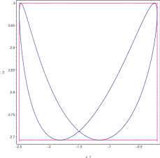
(a) $\tilde{\wp}_{*}=-8.0$

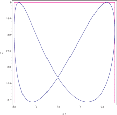
(b) $\tilde{\wp}_{*}=-11.0$

Figure 5.1: Generic polhodes in $S\subset{\mathbb{R}}^{2}=(z_{1},z_{2})$.

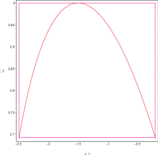
(a) $\tilde{\wp}_{*}=-\infty$

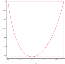
(b) $\tilde{\wp}_{*}=E_{1}=-7.2$

Figure 5.2: Special polhodes in $S$.

Closed geodesics related to 3:1 covering.

Under the the projective transformation (3.5) with $\beta=b_{1}=-\sqrt{3g_{2}}$, the branch points $\{-\sqrt{3g_{2}},3e_{1},3e_{2},3e_{3},\sqrt{3g_{2}},\infty\}$ of the curve $G$ transform to infinity, 4 positive numbers $\{a_{1},a_{2},a_{3},c\}$ and zero respectively. Given $g_{2},e_{1}$, the parameters $e_{2},e_{3}$ of the elliptic curve are defined uniquely:

$$e_{2}=-\frac{e_{1}}{2}-\frac{\sqrt{3}}{6}R,\quad e_{3}=-\frac{e_{1}}{2}+\frac{\sqrt{3}}{6}R,\qquad R=\sqrt{3g_{2}-9e_{1}^{2}}.$$

Then, assuming that $a_{1}<a_{2}<c<a_{3}$, we get

$$a_{3} =\frac{1}{3e_{1}+B},\quad a_{1}=\frac{1}{2B},$$

$$a_{2} =\frac{1}{3e_{3}+B}\equiv\frac{2}{(6e_{3}-B)^{2}}\left(2B-3e_{3}-\sqrt{3}R\right),$$ (5.12)

$$c =\frac{1}{3e_{2}+B}\equiv\frac{2}{(6e_{3}-B)^{2}}\left(2B-3e_{3}+\sqrt{3}R\right),$$

where $B=\sqrt{3g_{2}}$. As a result, the four parameters $a_{1}<a_{2}<c<a_{3}$ are uniquely defined by $g_{2}$ (or $B$) and $e_{1}$.

Now we apply the transformation (4.14) with $b_{1}=-\sqrt{3g_{2}}$ to the polhode (5.7). This yields an equation of a closed geodesic on $Q$ written in terms of the symmetric functions $\Sigma_{1}=\lambda_{1}+\lambda_{2}$, $\Sigma_{2}=\lambda_{1}\lambda_{2}$ of the ellipsoidal coordinates. (In fact, one obtains a family of such geodesics parameterized by $\tilde{\wp}_{*}$.) Then, making the substitution (4.15) one obtains the equation of the cylinder cutting surface ${\cal V}_{\tilde{\wp}_{*}}$ in terms of squares of the Cartesian coordinates $X_{1},X_{3}$. For a generic parameter $\tilde{\wp}_{*}$ this equation has degree 12, it is quite tedious and we do not give it here. However, the structure of a generic polhode in $S\subset(z_{1},z_{2})$ and the correspondence between the sets $\{3e_{1},3e_{2},3e_{3},\sqrt{3g_{2}}\}$ and $\{a_{1},a_{2},c,a_{3}\}$ is already sufficient to give a complete qualitative description of the geodesic on $Q$.

Namely, let ${\cal R}_{c}$ be a ring on $Q$ bounded by the two connected components of the caustic $Q\cap Q_{c}$ and $\rho=k:l\in{\mathbb{Q}}$ be the quotient of the numbers of complete rotations performed by a closed geodesics in lateral and meridional directions on the ring respectively (the rotation number).

Theorem 5.1.

1). Under the assumption $a_{1}<a_{2}<c<a_{3}$, the geodesic corresponding to a generic polhode (5.7) or to the special polhodes is located in the ring ${\cal R}_{c}$ between planes $X_{3}=\pm h$, $h<\sqrt{a_{3}}$ and has rotation number $\rho=2:1$. It touches the caustic $Q\cap Q_{c}$ at 2 points and has one self-intersection.

2). Under the assumption $a_{1}<c<a_{2}<a_{3}$, the geodesic is located in the ring ${\cal R}_{c}$ between planes $X_{1}=\pm h$, $h<\sqrt{a_{1}}$ and has rotation number $1:2$. It touches the caustic $Q\cap Q_{c}$ at 4 points and has no self-intersections.

In both cases the geodesic is either a 2-fold covering of the real asymmetric part of a generic polhode ${\cal H}_{\tilde{\wp}_{*}}$ or a 4-fold covering of that of the special polhodes.

Note that the self-intersection point of the polhode does not correspond to the self-intersection point of the corresponding closed geodesic.

Sketch of Proof of Theorem 5.1. Under the projective transformation (4.14), a polhode ${\cal H}_{\tilde{\wp}_{*}}\subset(z_{1},z_{2})$ is mapped to a polhode $\widetilde{\cal H}_{\tilde{\wp}_{*}}$ in ${\mathbb{R}}^{2}=(\lambda_{1},\lambda_{2})$, which is tangent to lines $\lambda_{j}=a_{i}$, $i=1,2,3$ and $\lambda_{j}=c$. In view of relations (2.1), the point of tangency of $\widetilde{\cal H}_{\tilde{\wp}_{*}}$ to the line $\lambda_{j}=a_{i}$ corresponds to the moment when the geodesic $X(s)$ on $Q$ crosses the plane $X_{i}=0$, and the tangency to the line $\lambda_{j}=c$ corresponds to the tangency of $X(s)$ to the caustic $Q\cap Q_{c}$. Estimating ordering and number of the tangencies of $\widetilde{\cal H}_{\tilde{\wp}_{*}}$ in the cases $a_{2}<c$ and $c<a_{2}$, one arrives at the statements of the theorem. $\boxed{}$

An Example of a Generic Closed Geodesic.

For the above numerical choice of $g_{2},g_{3}$ one gets $B=3$, $e_{1}=-0.83054$, $e_{2}=-0.067069$, $e_{3}=0.89761$ and the formulas (5.12) (or the images of the values in (5.10)) yield

$$a_{1}=0.16667,\quad a_{2}=0.1776,\quad c=0.3579,\quad a_{3}=1.96703.$$

(This means that the corresponding ellipsoid is almost ”prolate”.) Projections of the intersection $Q\cap{\mathcal{V}}_{\wp}$ onto $(X_{1},X_{3})$- and $(X_{1},X_{2})$-planes for $\tilde{\wp}_{*}=-11$ are given in Figure 5.3.

One can see that this intersection actually consists of four closed geodesics obtained from each other by reflections $(X_{1},X_{2})\mapsto(\pm X_{1},\pm X_{2})$. Each geodesics has the only self-intersection point at $X_{3}=0$ and corresponds to the polhode in Figure 5.1 (b) which is passed two times.

It is natural to conjecture that the four geodesics are real parts of one and the same spatial elliptic curve which are obtained from each other via translations by elements of a finite order subgroup of the curve.

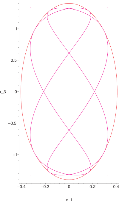
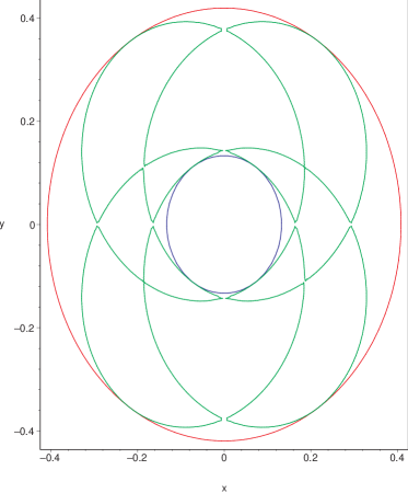
Figure 5.3: Projection of four symmetrically related closed geodesics onto $(X_{1},X_{3})$ and $(X_{1},X_{2})$-planes for $\tilde{\wp}_{*}=-11$. In the latter case the projection of the common caustic is indicated.

Special Geodesic for ${\mathcal{H}}_{\infty}$.

In the special case $\tilde{\wp}_{*}=\infty$ the equation of the surface ${\mathcal{V}}_{\wp}$ simplifies drastically and admits the following factorization

$$\left(\alpha(X_{1}-\gamma)^{2}+\beta X_{3}^{2}-\delta\right)\cdot\left(\alpha\left(X_{1}+\gamma\right)^{2}+\beta X_{3}^{2}-\delta\right)=0,$$ (5.13)

where

$$\alpha =\frac{\sqrt{2}}{9}\left(B-6e_{1}\right)(\left(2B+3e_{1}\right)-\sqrt{3}R),$$ (5.14)

$$\beta =\frac{1}{3\sqrt{6}}\left(B+3e_{1}\right)\;\left(R-3\sqrt{3}e_{1}\right),$$

$$\gamma =-\frac{2}{9\alpha}\left(R+3\sqrt{3}e_{1}\right)R\sqrt{B},$$

$$\delta =-\frac{B^{2}}{3\sqrt{2}}\frac{\left(R+3\sqrt{3}e_{1}\right)^{2}}{\left(\sqrt{3}R-\left(3e_{1}+2B\right)\right)\left(B-6e_{1}\right)}\,.$$

and, as above, $B=\sqrt{3g_{2}}$, $R=\sqrt{3g_{2}-9e_{1}^{2}}$.

Equation (5.13) defines a union of two elliptic cylinders in ${\mathbb{R}}^{3}$ that are transformed to each other by mirror symmetry with respect to the plane $X_{1}=0$. It appears that each cylinder is tangent to the ellipsoid $Q$ at a point $(X_{2}=X_{3}=0)$ and cuts out a closed geodesic with the only self-intersection at this point. As a result, the special closed geodesic on $Q$ related to the polhode (5.8) is defined by its intersection with just a quadratic surface defined by one of the two factors in (5.13)).

Remark.

Note that due to the self-intersection, the special geodesic in ${\mathbb{R}}^{3}$ (${\mathbb{P}}^{3}$) is a rational algebraic curve and not an elliptic one, as the intersection of two generic quadrics. It admits parameterization

$$X_{1}=d+h_{1}\cos(2\nu),\quad X_{2}=h_{2}\sin(2\nu),\quad X_{3}=h_{3}\sin\nu,\qquad\nu\in{\mathbb{R}},$$

$h_{i},d$ being certain constants.

On the other hand, in the phase space $(X,\dot{X})$ the corresponding periodic solution has no self-intersections and represents an elliptic curve. Indeed, in view of formulas (2.1), the latter can be regarded as a 4-fold covering of the rational special polhode (5.8). The covering has simple ramifications at 8 points that are projected to two vertices of the domain $S$ and two vertices of the symmetric domain $S^{\prime}$ obtained by reflection with respect to the diagonal $z_{1}=z_{2}$. Then, according to the Riemann–Hurwitz formula (see, e.g., [3]), the covering has genus one. The projection ${\mathbb{C}}^{6}=\{(X,\dot{X})\}\mapsto{\mathbb{C}}^{3}=\{X\}$ maps two different points of the elliptic solution to the self-intersection point on $Q$.

For the above values of the parameters $a_{1},a_{2},a_{3},c$ the 3D graph of the special geodesic is shown in Figure 5.4.

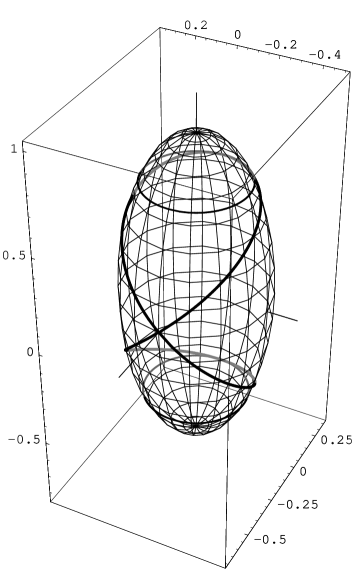
Figure 5.4: Two 3D Images of the Special Geodesic Corresponding to ${\cal H}_{\infty}$.

Special Geodesic for ${\mathcal{H}}_{E_{1}}$.

Applying the transformation (4.14) with $b_{1}=-\sqrt{3g_{2}}$ to the special polhode (5.9) and making the substitution (4.15) we arrive at a sextic surface in ${\mathbb{R}}^{3}$ given by equation

$$-256B^{3}f_{1}^{3}X_{1}^{6}-\left(48B^{3}f_{1}f_{2}^{2}+432Be_{1}^{2}f_{1}f_{2}^{2}+288B^{2}e_{1}f_{1}f_{2}^{2}\right)X_{1}^{2}X_{3}^{4}$$

$$+\left(2304B^{3}e_{1}f_{1}^{2}-192B^{4}f_{1}^{2}-6912B^{2}e_{1}^{2}f_{1}^{2}\right)X_{1}^{4}$$

$$+\left(192B^{4}f_{1}f_{2}+5184Be_{1}^{3}f_{1}f_{2}-864B^{3}e_{1}f_{1}f_{2}-2592B^{2}e_{1}^{2}f_{1}f_{2}\right)X_{1}^{2}X_{3}^{2}$$

$$+\left(-4B^{3}f_{2}^{3}-108e_{1}^{3}f_{2}^{3}-108Be_{1}^{2}f_{2}^{3}-36B^{2}e_{1}f_{2}^{3}\right)X_{3}^{6}$$

$$+\left(3B^{5}f_{2}-11\,664e_{1}^{5}f_{2}-27B^{4}e_{1}f_{2}+1296B^{2}e_{1}^{3}f_{2}-108B^{3}e_{1}^{2}f_{2}\right)X_{3}^{2}$$

$$+\left(864B^{4}e_{1}f_{1}-46\,656Be_{1}^{4}f_{1}-36B^{5}f_{1}+31\,104B^{2}e_{1}^{3}f_{1}-7776B^{3}e_{1}^{2}f_{1}\right)X_{1}^{2}$$

$$+\left(1944e_{1}^{4}f_{2}^{2}-12B^{4}f_{2}^{2}+648Be_{1}^{3}f_{2}^{2}-144B^{3}e_{1}f_{2}^{2}-324B^{2}e_{1}^{2}f_{2}^{2}\right)X_{3}^{4}$$

$$-\left(192B^{3}f_{1}^{2}f_{2}+576B^{2}e_{1}f_{1}^{2}f_{2}\right)X_{1}^{4}X_{3}^{2}=0,$$ (5.15)

where

$$f_{1}=\left(9e_{1}^{2}-\frac{7}{4}B^{2}+BR\sqrt{3}\right),\quad f_{2}=\left(27e_{1}^{2}-\frac{3}{2}B^{2}-9Be_{1}+BR\sqrt{3}+3Re_{1}\sqrt{3}\right).$$

It cuts out a pair of closed geodesic on $Q$ that are transformed to each other by mirror symmetry with respect to the plane $X_{2}=0$. Both geodesics have a 3D shape similar to that in Figure 5.4, each of them has the only self-intersection point for $(X_{1}=X_{3}=0)$.

Note, however, that in contrast to quartic equation (5.13), the sextic polynomial in (5.15) does not admit a factorization, hence none of the above geodesics can be represented as the intersection of $Q$ with a quadratic or a cubic cylinder.

For the above choice of moduli $g_{2},g_{3}$ and the parameters $a_{i},c$ the projection of the sextic surface and the corresponding geodesics onto $(X_{1},X_{3})$-plane are given in Figure 5.5.

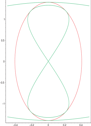
Figure 5.5: Projection of the sextic surface (5.15) and the geodesic for ${\cal H}_{E_{1}}$ onto $(X_{1},X_{3})$-plane.

Remark.

As follows from the above considerations, under the condition $a_{1}<a_{2}<c<a_{3}$ all the real closed geodesics of the one-parametric family have one self-intersection point on the equator $\{X_{3}=0\}\subset Q$, and as the parameter $\tilde{\wp}_{*}$ ranges from $-\infty$ to $E_{1}$, this point varies from the $X_{1}$-axis to $X_{2}$-axis.

The case $a_{1}<c<a_{2}<a_{3}$ will be illustrated in detail elsewhere.

6 The case of 4:1 tangential covering

This case was originally studied by Darboux and later appeared in paper [16] in connection with new elliptic solutions of the KdV equation (see also [17, 15]). Namely, the genus 2 curve $G$

$$w^{2}=-(z-6e_{1})\prod_{l=1}^{4}(z-z_{l}),$$ (6.1)

with

$$z_{1,2} =e_{3}+2e_{2}\pm\sqrt{28e_{2}^{2}+76e_{2}e_{3}+40e_{3}^{2}},$$

$$z_{3,4} =e_{2}+2e_{3}\pm\sqrt{28e_{3}^{2}+76e_{2}e_{3}+40e_{2}^{2}},$$

is a 4-fold cover of the curve (3.2). It also covers second elliptic curve
${\cal E}_{2}=\left\{W^{2}=-4(Z-E_{1})(Z-E_{2})(Z-E_{3})\right\}$, such that

$$E_{1} =3\left(e_{2}-e_{3}\right)^{3}-6\left(e_{2}-e_{1}\right)(5e_{1}-2e_{3})^{2},$$

$$E_{2} =-6\left(e_{2}-e_{3}\right)^{3}+3\left(e_{2}-e_{1}\right)(5e_{1}-2e_{3})^{2},$$ (6.2)

$$E_{3} =3\left(e_{2}-e_{3}\right)^{3}+3\left(e_{2}-e_{1}\right)(5e_{1}-2e_{3})^{2}$$

as described by one of the formulas

$$Z =E_{1}+F_{\alpha}(z),\quad F_{\alpha}=\frac{9}{4}\frac{\left(z^{2}-3e_{\alpha}z-24\left(e_{\beta}^{2}+e_{\gamma}^{2}\right)-51e_{\beta}e_{\gamma}\right)^{2}}{z-6e_{\alpha}},$$ (6.3)

$$W =-w\frac{dZ(z)}{dz},$$

where $(\alpha,\beta,\gamma)$ is a circular permutation of $(1,2,3)$. In the sequel we assume
$\alpha=1,\beta=2,\gamma=3$.

Substituting projection formulas (6.3) to the generating equation (4.8) one obtains equation of generic polhodes of degree 16, which is much more tedious than the family (5.7) for the 3:1 cover, so we do not give it here.

The special polhodes for $\tilde{\wp}_{*}=\infty$ and $\tilde{\wp}_{*}=E_{1}$.

Substituting projection formulas (6.3) to the special generating equation (4.11), we obtain algebraic equation of degree 4,

$$6e_{1}\left(z_{1}^{3}+z_{2}^{3}\right)-36e_{1}^{2}\left(z_{1}^{2}+z_{2}^{2}\right)-z_{1}^{2}z_{2}^{2}+\left(12e_{1}(z_{1}+z_{2})-z_{1}^{2}-z_{2}^{2}\right)z_{2}z_{1}$$

$$+(6e_{2}e_{3}+3e_{1}^{2})z_{1}z_{2}+\left(54e_{1}^{3}-612e_{1}e_{2}e_{3}-288e_{1}e_{2}^{2}-288e_{1}e_{3}^{2}\right)(z_{1}+z_{2})$$

$$+9\left(17e_{2}e_{3}+8e_{2}^{2}+8e_{3}^{2}\right)\left(17e_{2}e_{3}+12e_{1}^{2}+8e_{2}^{2}+8e_{3}^{2}\right)=0\,.$$ (6.4)

Next, substituting (6.3) into the special generating equation (4.13) with $E_{\alpha}=E_{1}$ and taking into account relation $E_{1}+E_{2}+E_{3}=0$, one gets the following equation of degree 8

$$81\,z_{1}^{4}\,z_{2}^{4}-486e_{1}(z_{2}^{3}\,z_{1}^{4}+z_{2}^{4}\,z_{1}^{3})-({3159}\,e_{2}^{2}+6804\,{e_{2}}\,{e_{3}}+{3159}\,{e_{3}}^{2})\,(z_{2}^{2}\,z_{1}^{4}+z_{2}^{4}\,z_{1}^{2})$$

$$+2916\,e_{1}^{2}\,z_{1}^{3}z_{2}^{3}+2916\,e_{1}\xi_{1}(z_{2}\,z_{1}^{4}+z_{2}^{4}\,z_{1})+1458\,e_{1}\xi_{2}\,(z_{2}^{2}\,z_{1}^{3}+z_{2}^{3}\,z_{1}^{2})$$

$$+729\,\xi_{1}^{2}\,(z_{1}^{4}+z_{2}^{4})-8748\,\xi_{1}\,e_{1}^{2}\,(z_{2}\,z_{1}^{3}+z_{2}^{3}\,z_{1})+729\,\xi_{2}^{2}\,z_{1}^{2}\,z_{2}^{2}-4374e_{1}\xi_{1}^{2}\,(z_{1}^{3}+z_{2}^{3})$$

$$-4374\,e_{1}\xi_{1}\xi_{2}\,(z_{2}\,z_{1}^{2}+z_{2}^{2}\,z_{1})-2187\,\xi_{2}\,\xi_{1}^{2}\,(z_{1}^{2}+z_{2}^{2})+16\bigg{(}104976\,{e_{2}}^{6}+656100\,{e_{2}}^{5}\,{e_{3}}$$

$$+\frac{6725025}{4}\,{e_{2}}^{4}\,{e_{3}}^{2}+\frac{4520529}{2}\,{e_{2}}^{3}\,{e_{3}}^{3}+\frac{6725025}{4}\,{e_{2}}^{2}\,{e_{3}}^{4}+656100\,{e_{2}}\,{e_{3}}^{5}+104976\,{e_{3}}^{6}-2\,{E_{2}}^{2}$$

$$-5\,{E_{2}}\,{E_{3}}-2\,{E_{3}}^{2}\bigg{)}z_{1}\,z_{2}+\frac{3}{8}e_{1}(1119744\,{e_{2}}^{6}+7138368\,{e_{2}}^{5}\,{e_{3}}+18528264\,{e_{2}}^{4}\,{e_{3}}^{2}$$

$$+25021467\,{e_{2}}^{3}\,{e_{3}}^{3}+18528264\,{e_{2}}^{2}\,{e_{3}}^{4}+7138368\,{e_{2}}\,{e_{3}}^{5}+1119744\,{e_{3}}^{6}+32\,{E_{2}}^{2}$$

$$+80\,{E_{2}}\,{E_{3}}+32\,{E_{3}}^{2})(z_{1}+z_{2})+52225560\,e_{2}^{6}\,e_{3}^{2}+107298594\,e_{2}^{5}e_{3}^{3}+\frac{2165451489}{16}\,e_{2}^{4}e_{3}^{4}$$

$$+14276736\,{e_{2}}^{7}\,{e_{3}}-144\,{e_{2}}\,{e_{3}}\,{E_{3}}^{2}-72\,{e_{3}}^{2}\,{E_{2}}^{2}-180\,{e_{3}}^{2}\,{E_{2}}\,{E_{3}}-72\,{e_{3}}^{2}\,{E_{3}}^{2}$$

$$+107298594\,{e_{2}}^{3}\,{e_{3}}^{5}+52225560\,{e_{2}}^{2}\,{e_{3}}^{6}+14276736\,e_{2}e_{3}^{7}+1679616\,{e_{3}}^{8}-72\,{e_{2}}^{2}\,{E_{2}}^{2}$$

$$-180\,{e_{2}}^{2}\,{E_{2}}\,{E_{3}}-72\,{e_{2}}^{2}\,{E_{3}}^{2}-144\,{e_{2}}\,{e_{3}}\,{E_{2}}^{2}-360\,{e_{2}}\,{e_{3}}\,{E_{2}}\,{E_{3}}+1679616\,{e_{2}}^{8}=0,$$ (6.5)

$$\xi_{1}=8\,{e_{2}}^{2}+17\,{e_{2}}\,{e_{3}}+8\,{e_{3}}^{2},\quad\xi_{2}=13\,{e_{2}}^{2}+28\,{e_{2}}\,{e_{3}}+13\,{e_{3}}^{2},$$

Examples of polhodes in $S$.

To illustrate the above polhodes, in the first elliptic curve (3.2) we choose

$$e_{1}=-2,\quad e_{2}=-1,\quad e_{3}=3,\mbox{ so that }\quad E_{1}=-1728,\quad E_{2}=1152,\quad E_{3}=576,$$

and the roots of the polynomial in (6.1) become

$$(-12.0,\;-11.649,\;-3.0,\;13.0,\;13.649).$$ (6.6)

As a result, the square domain $S\subset(z_{1},z_{2})$ where the corresponding variables $w_{1},w_{2}$ are real is

$$S=\{-11.649\leq z_{1}\leq-3.0,\quad 13.0\leq z_{2}\leq 13.649\}.$$ (6.7)

If the parameter $\tilde{\wp}_{*}$ ranges in the interval $(-\infty;E_{1}=-1728)$, then the conditions (4.10) do not hold in $S$, hence the real asymmetric part of the polhode is non-empty.

Graphs of polhodes in the domain (6.7) for a generic value of $\tilde{\wp}_{*}\in(-\infty;-1728)$ is given in Figure 6.2, whereas the special polhodes defined by (6.4) and (6.5) are shown in Figure 6.2.

As seen from Figure 6.2, the generic polhodes in $S$ intersect generic lines $z_{2}=$const and $z_{1}=$const at 6 and 2 points respectively.

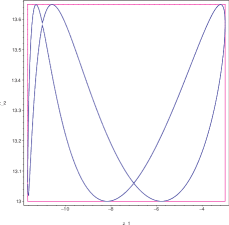
(a) $\tilde{\wp}_{*}=-4900$

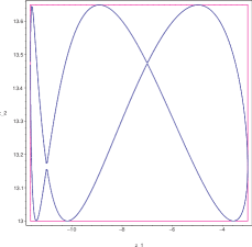
(b) $\tilde{\wp}_{*}=-7000$

Figure 6.1: Generic polhodes in $S\subset{\mathbb{R}}^{2}=(z_{1},z_{2})$

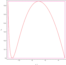
(a) $\tilde{\wp}_{*}=-\infty$

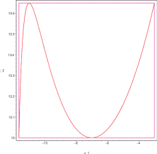
(b) $\tilde{\wp}_{*}=-1728$

Figure 6.2: Special polhodes.

Special Closed Geodesic for ${\cal H}_{\infty}$.

Assuming, as above, $e_{1}<e_{2}<e_{3}$, we conclude that $b_{1}=-6e_{1}$ is the minimal root of the hyperelliptic polynomial in (6.1). Setting this value into the transformation (4.14), we get

$$z_{1}=\frac{6e_{1}\lambda_{1}+1}{\lambda_{1}},\quad z_{2}=\frac{6e_{1}\lambda_{2}+1}{\lambda_{2}}.$$

The latter substitution transforms equation (6.4) of polhode ${\cal H}_{\infty}$ to

$$\left(102e_{2}e_{3}-117e_{1}^{2}+48e_{2}^{2}+48e_{3}^{2}\right)\lambda_{1}^{2}\lambda_{2}^{2}-\lambda_{1}^{2}-\lambda_{2}^{2}-\lambda_{1}\lambda_{2}$$

$$\quad-18e_{1}\left(\lambda_{1}+\lambda_{2}\right)\lambda_{2}\lambda_{1}+9\left(17e_{2}e_{3}-6e_{1}^{2}+8e_{2}^{2}+8e_{3}^{2}\right)^{2}\,\lambda_{1}^{3}\lambda_{2}^{3}=0,$$ (6.8)

which describes the closed geodesic in ellipsoidal coordinates on $Q$. Next, assuming that $a_{1}<a_{2}<c<a_{3}$, we find

$$a_{1}=\frac{1}{6e_{1}+e_{2}+2e_{3}+\sqrt{28e_{3}^{2}+76e_{2}e_{3}+40e_{2}^{2}}},\quad a_{2}=\frac{1}{6e_{1}+e_{2}+2e_{3}-\sqrt{28e_{3}^{2}+76e_{2}e_{3}+40e_{2}^{2}}},$$

$$a_{3}=\frac{1}{6e_{1}+e_{3}+2e_{2}-\sqrt{28e_{2}^{2}+76e_{2}e_{3}+40e_{3}^{2}}},\quad c=\frac{1}{6e_{1}+e_{3}+2e_{2}+\sqrt{28e_{2}^{2}+76e_{2}e_{3}+40e_{3}^{2}}}.$$

Applying formulas (4.15) and simplifying, one obtains equation of cylinder surface ${\cal V}_{\infty}$ of degree 6 in coordinates $(X_{1},X_{3})$, which admits the factorization

$$F_{-}(X_{1},X_{3})\,F_{+}(X_{1},X_{3})=0,$$

$$F_{\pm}=\pm h_{30}X_{1}^{3}+h_{03}X_{3}^{3}+h_{21}X_{1}^{2}X_{3}\pm h_{12}X_{1}X_{3}^{2}\pm h_{10}X_{1}+h_{01}X_{3},$$ (6.9)

where $h_{ij}$ are rather complicated expressions of $e_{2},e_{3}$, so we do not give them here.

Thus ${\cal V}_{\infty}$ is a union of two cubic cylinders ${\cal V}_{\infty-}$, ${\cal V}_{\infty+}$ that are obtained from each other by mirror symmetry with respect to the plane $X_{1}=0$.

Example of a closed geodesic for ${\cal H}_{\infty}$.

Under the above assumption $a_{1}<a_{2}<c<a_{3}$, the values (6.6) lead to numbers

$$a_{1}=3.69877\times 10^{-2},\quad a_{2}=0.04,\quad c=0.111111,\quad a_{3}=2.84981$$

and the equation of the cylinder ${\cal V}_{\infty+}$ becomes

$$-0.301917X_{1}^{3}-0.470556X_{1}X_{3}^{2}+0.652885X_{1}^{2}X_{3}+1.87228X_{1}-0.303831X_{3}+0.113051X_{3}^{3}=0.$$ (6.10)

Its projection onto $(X_{1},X_{3})$-plane and the 3D graph of the corresponding geodesic are shown in Figure 6.3 . The cylinder is tangent to the ellipsoid $Q$ at 2 points with $X_{2}=0$, which implies that the geodesic has two self-intersection points.

Remark.

The special geodesic can be regarded as a two-fold covering of the plane algebraic curve ${\mathcal{F}}_{\pm}=\{F_{\pm}(X_{1},X_{3})=0\}$, which is ramified at two points of transversal intersection of ${\mathcal{F}}_{\pm}$ with the ellipse $\{X_{1}^{2}/a_{1}+X_{3}^{2}/a_{3}=1\}$. (There is no ramification at the two points of tangency with the ellipse.) Using explicit expressions of (6.9), one can show that for any value of $e_{2},e_{3}$ the genus of ${\mathcal{F}}_{\pm}$ equals zero. Hence, according to the Riemann–Hurvitz formula, the special closed geodesic is a rational curve.

However, similarly to the special geodesic for the 3:1 covering, in the phase space $(X,\dot{X})$ the periodic solution corresponding to ${\cal H}_{\infty}$ has no self-intersections and represents a connected component of real part of an elliptic curve.

General closed geodesics.

For a generic parameter $\tilde{\wp}_{*}$ the equation of the cutting cylinder ${\cal V}_{\tilde{\wp}_{*}}$ has degree 16 and its projection onto $(X_{1},X_{3})$-plane looks quite tangled: it includes 2 intersecting closed geodesics obtained from each other by reflections $X_{1}\mapsto-X_{1}$. The structure of the real asymmetric part of generic and the special polhodes implies the following behavior under the condition $a_{1}<a_{2}<c<a_{3}$: all the closed geodesics of the family have two centrally symmetric self-intersection points and as the parameter $\tilde{\wp}_{*}$ ranges from $-\infty$ to $E_{1}$, these points vary from the plane $\{X_{2}=0\}$ to $\{X_{1}=0\}$. All the geodesics have rotation number $\rho=3:1$.

Similarly to the case of the 3-fold tangential covering, one can consider the ordering
$a_{1}<c<a_{2}<a_{3}$, which leads to generic and special closed geodesics on $Q$ without self-intersections.

,  

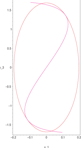
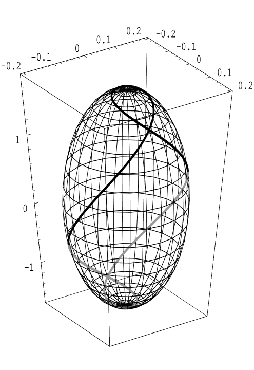
Figure 6.3: Projection of the cylinder ${\cal V}_{\infty+}$ onto $(X_{1},X_{3})$-plane and Special Geodesic for ${\cal H}_{\infty}$.

Conclusion

In this paper we proposed a simple method of explicit constructing families of algebraic closed geodesics on triaxial ellipsoids, which is based on properties of tangential coverings of an elliptic curve and the addition theorem for elliptic functions. We applied the method to the cases of 3- and 4-fold coverings and gave concrete examples of algebraic surfaces that cut such closed geodesics. The latter coincide with those obtained by direct numeric integration of the geodesic equation. This serves as an ultimate proof of correctness of the method. Depending on how one chooses the caustic parameter $c$ in the interval $(a_{1},a_{3})$, the closed geodesics may or may not have self-intersections.

Thus, our approach can be regarded as a useful application of the Weierstrass–Poincaré reduction theory. One must only know explicit covering formulas (4.2), as well as expressions for $z$-coordinates of the finite branch points of the genus 2 curve $G$ in terms of the moduli $g_{2},g_{3}$. To our knowledge, until now such expressions are calculated only for $N\leq 8$.

Since the method essentially uses the algebraic addition law on the second elliptic curve ${\mathcal{E}}_{2}$, it does not admit a straightforward generalization to similar description of algebraic closed geodesics on $n$-dimensional ellipsoids: as mentioned in Section 3, in this case ${\mathcal{E}}_{2}$ is replaced by an Abelian subvariety ${\mathcal{A}}_{n-1}$, for which an algebraic description is not known.

On the other hand, one should not exclude the existence of algebraic closed geodesics on ellipsoids related to other type of doubly periodic solutions of the KdV equation, e.g., elliptic not $x$, but in $t$-variable. This is expected to be a subject of a separate study.

Our approach can equally be applied to describe elliptic solutions of other integrable systems linearized on two-dimensional hyperelliptic Jacobians or their coverings.

Acknowledgments

I am grateful to A. Bolsinov, L. Gavrilov, V. Enolskii, E. Previato, and A. Treibich for stimulating discussions, as well as to A. Perelomov for some important suggestions during preparation of the manuscript and indicating me the reference [5]. I also thank the referees for their valuable remarks that helped to improve the text.

The support of grant BFM 2003-09504-C02-02 of Spanish Ministry of Science and Technology is gratefully acknowledged.

References

- [1] Abenda, S., Fedorov, Yu. Closed Geodesics and Billiards on Quadrics related to elliptic KdV solutions. Preprint. nlin.SI/0412034
- [2] Audin M. Courbes algébriques et systèmes intégrables: géodésiques des quadriques. Expo. Math. 12, no.3 (1994), 193–226
- [3] Belokolos E.D., Bobenko A.I., Enol’sii V.Z., Its A.R., and Matveev V.B. Algebro-Geometric Approach to Nonlinear Integrable Equations. Springer Series in Nonlinear Dynamics. Springer–Verlag 1994.
- [4] Belokolos E.D., Enol’ski V.Z. Reductions of theta-functions and elliptic finite-gap potentials. Acta Appl. Math. 36, (1994), 87–117
- [5] von Braunmühl A. Notiz über geodätische Linien auf den dreiaxigen Flächen zweiten Grades welche durch elliptische Functionen dargestellen lassen. Math. Ann., 26 (1886), 151–153
- [6] Dragovic, V., Radnovic, M. On periodical trajectories of the billiard systems within an ellipsoid in and generalized Cayley’s condition. J. Math. Phys. 39, No. 11, (1998), 5866–5869
- [7] Dragovic V., Radnovic M. Cayley-type conditions for billiards within quadrics in . ArXiv:math-ph/0503053
- [8] Hermite C. Oeuvres de Charles Hermite. Vol. III, Gauthier–Villars, Paris, 1912.
- [9] Jacobi K.G. Vorlesungen über Dynamik, Supplementband. Berlin. 1884
- [10] Knörrer H. Geodesics on the ellipsoid. Invent. Math. 59 (1980), 119–143
- [11] Knörrer H. Geodesics on quadrics and a mechanical problem of C.Neumann. J. Reine Angew. Math. 334 (1982), 69–78
- [12] Krazer A.: Lehrbuch der Thetafunctionen. Leipzig, Teubner, 1903. New York: Chelsea Publ.Comp. 1970
- [13] Krichiver I.M. Elliptic solutions of the Kadomcev-Petviasvili equations, and integrable systems of particles. (Russian) Funktsional. Anal. i Prilozhen. 14 (1980), no. 4, 45–54,95.
- [14] Previato, E. Poncelet theorem in space. Proc. Amer. Math. Soc. 127 (1999), no. 9, 2547–2556
- [15] A. O. Smirnov. Finite-gap elliptic solutions of the KdV equation. Acta Appl. Math. 36, (1994), 125–166
- [16] Treibich A. and Verdier J. L. Tangential covers and sums of 4 triangular numbers. C. R. Acad. Sci. Paris 311, (1990), 51–54
- [17] Treibich A. Hyperelliptic tangential covers, and finite-gap potentials. (Russian) Uspekhi Mat. Nauk 56 (2001), no. 6(342), 89–136; translation in Russian Math. Surveys 56 (2001), no. 6, 1107–1151
- [18] Weierstrass K. Über die geodätischen Linien auf dem dreiachsigen Ellipsoid. In: Mathematische Werke I, 257–266