Phenomenology of Wall Bounded Newtonian Turbulence

Abstract

We construct a simple analytic model for wall-bounded turbulence, containing only four adjustable parameters. Two of these parameters characterize the viscous dissipation of the components of the Reynolds stress-tensor and other two parameters characterize their nonlinear relaxation. The model offers an analytic description of the profiles of the mean velocity and the correlation functions of velocity fluctuations in the entire boundary region, from the viscous sub-layer, through the buffer layer and further into the log-layer. As a first approximation, we employ the traditional return-to-isotropy hypothesis, which yields a very simple distribution of the turbulent kinetic energy between the velocity components in the log-layer: the streamwise component contains a half of the total energy whereas the wall-normal and the cross-stream components contain a quarter each. In addition, the model predicts a very simple relation between the von-Kármán slope $\kappa$ and the turbulent velocity in the log-law region $v^{+}$ (in wall units): $v^{+}=6\kappa$. These predictions are in excellent agreement with DNS data and with recent laboratory experiments.

Introduction

The tremendous amount of work devoted to understanding the apparent experimental deviations from the classical phenomenology of homogeneous and isotropic turbulence MY ; Fri tends to obscure the fact that in many respects this phenomenology is almost right on the mark. Starting with the basic ideas of Richardson and Kolmogorov, and continuing with a large number of ingenious closures, one can offer a reasonable set of predictions regarding the statistical properties of the highly complex phenomenon of homogenous and isotropic turbulence. Thus one predicts the range of scales for which viscous effects are negligible (the so called “inertial range” of turbulence), the cross over scale below which dissipative effects are crucial (also known as the “Kolmogorov scale”), the exact form of the third order structure function $S_{3}(R)$ (third moment of the longitudinal velocity difference across a scale $R$), including numerical pre-factors, and an approximate form of structure function of other orders $S_{n}(R)$ (predicted to scale like $R^{n/3}$ but showing deviations in the scaling exponents which grow with the order, giving rise to much of the theoretical work alluded to above). In particular much effort was devoted to calculate the so called “Kolmogorov constant” $C_{2}$ which is the pre-factor of the second order structure function, with closure approximations (see, e.g. Refs. 66Kra ; 86YO ) coming reasonably close to its experimental estimate. Notwithstanding the deviations from the classical phenomenology, one can state that it provides a reasonable first order estimate on many non-trivial aspects of homogeneous and isotropic turbulence. In contrast, the phenomenological theory of wall bounded turbulence is less advanced. In reality most turbulent flows are bounded by one or more solid surfaces, making wall bounded turbulence a problem of paramount importance. Evidently, a huge amount of literature had dealt with problem, with much ingenuity and considerable success 00Pope . In particular one refers to von-Kármán’s log-law of the wall which describes the profile of the mean velocity as a function of the distance from the wall. It appears however that the literature lacks an analytically tractable model of wall bounded flows whose predictions can be trusted at a level comparable to the phenomenological theory of homogeneous turbulence.

In this paper we attempt to reduce this gap and offer as simple as possible but still realistic model (a ”minimal model”) for the viscous-to-turbulent flow in the entire region from the very surface through the logarithmic boundary layer (hereafter, log-layer) up to the upper boundary of outer turbulent region. Our final goal is to create clear physical grounds for improved description of the flow-surface interactions in numerical fluid-mechanics models (both engineering and geophysical) where the viscous and the buffer layers cannot be resoled and should be parameterized. To attain these ends we need to obtain analytical solutions (numerical solution would be of no use), which calls for simplification of the governing equations. Accordingly, our strategy is a pragmatic, task-dependent simplification and restrictions. In particular we concentrate on descriptions of the profile of mean flow and the statistics of turbulence on the level of simultaneous, one-point, second-order velocity correlation functions.In other words, the objects that we are after are the entries of the Reynolds-stress tensor as a function of the distance from the wall. The model will be presented for plain geometry; this geometry is relevant for a wide variety of turbulent flows, like channel and plain Couette flows, fluid flows over inclined planes under gravity (modelling river flows), atmospheric turbulent boundary layers over flat planes and, in the limit of large Reynolds numbers, many other turbulent flows, including pipe, circular Couette flows, etc.

Suggested in this paper phenomenological theory of wall-bounded flows is based on standard ideas 00Pope ; nevertheless we develop the theory slightly further than anything that exists currently in the literature. In our study we will stress analytical tractability; in other words, we will introduce approximations in order to achieve a model whose properties and predictions can be understood without resort to numerical calculations. Nevertheless we will show that the model appears very dependable in the sense that its predictions check very well in comparison to direct numerical simulations, including some rather non-trivial predictions that are corroborated only by very recent simulations and experiments (which only now reach the sufficient accuracy and high Reynolds numbers).

We should notice, that considering the mean velocity and the second-order statistics in these (neutrally stratified) flows, we neglect some mechanisms and features although present but not essential in the problem under consideration. However, proceeding further, in particular, to account for the density or temperature stratification (out of the scope of this paper), we quite probably will be forced to rule out of some simplifications acceptable in the first task and to account, for example, for a spacial energy flux and even for coherent structures.

In Sec. I we formulate a model which is a version of the “algebraic Reynolds-stress model” 00Pope . In Sec. I.1 we introduce notations and recall the equations describing the mechanical balance; in Sec. I.2 we state the assumptions and detail the approximations used in the context of the balance equations for the components of the Reynolds stress tensor $W_{ij}$. The result of these considerations is a set of 5 equations for the mean shear $S$ and $W_{ij}$ which is described in Sec. I.3. For actual calculations this set of equations is still too rich since it contains 12 adjustable parameter. Eight of these parameters control the nonlinear behavior of the system in the outer layer and four additional parameters govern the energy dissipation in the viscous sub-layer. Clearly, further reduction of the model is called for. This is accomplished in Sec. II. First, in Sec. II.1 we consider the full 12 parametrical solution of the model, and present a comparison with experimental observations in Sec. II.1.4. This comparison indicates that an adequate description of the entire turbulent boundary layer phenomenology can be achieved with only four parameters instead of twelve. We refer to the four-parameter model as the “minimal model”. In Sec. II.2 we reap the benefit of the minimal model: we find simple and physically transparent Eqs. (37) for the profiles of the Reynolds stress tensor $W_{ij}(y)$ and the mean shear $S(y)$ ($y$ is the distance from the wall) in terms of the root-mean-square turbulent velocity $v\equiv\sqrt{\mathstrut W_{ii}}$. Unfortunately, the equation for the $v(y)$ profile is quite cumbersome and cannot be solved analytically. Nevertheless we employ an effective iteration procedure that allows reaching highly accurate solutions with one or at most two iteration steps.

Section III is devoted to a comparison of the predictions of the minimal model with results of experiments and direct numerical simulations . In particular, in Sec. III.2 we show that the model describes the mean velocity profile in a channel flow with $1\%$-accuracy almost everywhere. Only in the core the model fails to describe so-called “velocity defect” (the upward deviation from the log-law) which is observed near the mid-channel (of about 5-6 units in $V^{+}$, independent on Reynolds number). For our purposes this mismatch in not essential. In Sec. III.3 we show that the minimal model provides a good qualitative description of kinetic energy profile, including position, amplitude and width of the peak of the kinetic energy in the buffer layer. In Sec. III.4 we show that with the same set of four parameters the model offers also a good qualitative description of the Reynolds stress profiles and the profiles of “partial” kinetic energies (in the streamwise, wall-normal and cross-stream directions) almost in the entire channel. The final Sec. IV presents a short summary of our results, including a discussion of the limitations of the minimal model. Possible improvements of the suggested model will have to start by addressing these limitations.

I Formulation of the model

Our starting point is the standard Reynolds decomposion 00Pope of the fluid velocity ${\bm{U}}(\bm{r},t)$ into its average (over time) ${\bm{V}}$ and the fluctuating components ${\bm{u}}$. In wall-bounded planar geometry the mean velocity is oriented in the (stream-wise) $\widehat{\bf{x}}$ direction, depending on the vertical (wall-normal) coordinate $y$ only:

$${\bm{U}}({\bm{r}},t)={\bm{V}}(y)+{\bm{u}}({\bm{r}},t)\ ,\quad{\bm{V}}(y)\equiv\langle{\bm{U}}({\bm{r}},t)\rangle=\widehat{\bf{x}}\,V(y)\ .$$ (1)

The mean velocity and the fluctuating parts are used to construct the objects of the theory which are the components of the Reynolds stress tensor ${\bm{W}}(y)$ and the mean shear:

$$W_{ij}(y)\equiv\left\langle u_{i}u_{j}\right\rangle\,,\quad S(y)\equiv\frac{dV(y)}{dy}\ .$$ (2)

We note that in previous applications 04LPPT ; 04DCLPPT ; 04BLPT ; 05LPPT ; 05LPPTa ; 04BDLPT ; 04LPT ; 05BCLLP ; 05BDLP we have employed a model in which only the trace of ${\bm{W}}(y)$ and its $xy$ component were kept in a simplified description. For the present purposes we consider all the component of this tensor, paying a price of having more equations to balance, but reaping the benefit of a significantly improved phenomenology. We discuss now the equations relating these variables to each other.

I.1 Equation for the mechanical balance

The first equation relates the Reynolds stress $W_{xy}$ to the mean shear; it describes the balance of the flux of mechanical momentum, it follows as an exact result from Navier-Stokes equations and has the familiar form:

$$-W_{xy}(y)+\nu_{0}S(y)=P(y)\ .$$ (3a)

$$W_{xy} \nu_{0}S(y) P(y) p^{\prime}=-dp/dx$$ on the left hand side (LHS) is the turbulent (reversible) contribution to the momentum flux whereas is the viscous (dissipative) contribution to the momentum flux. The RHS is the momentum flux, which may have different origin. For example, in a channel or pipe flow is generated by the pressure head. In the channel flow with the pressure gradient ,

$$P(y)=p^{\prime}(L-y)\,,$$ (3b)

where $L$ is the half width of the channel. In the pipe flow $P(y)$ is given by the same Eq. (3b) with $L$ being a half of the pipe radius. In a water flow over incline in the gravity field $p^{\prime}$ should be replaced by $g\sin a$, where $g$ is the gravity acceleration and $\alpha$ is the inclination angle. For Re${}_{\lambda}\gg 1$, near the wall one can neglect the $y$ dependence of $P(y)$, replacing $P(y)$ by its value at the wall: $P(y)\Rightarrow P_{0}\equiv P(0)$. Here the so-called “wall-based” Reynolds number Re_λ is defined by:

$$\mbox{Re}_{\lambda}\equiv\frac{L\sqrt{\mathstrut P(0)}}{\nu_{0}}\ .$$ (4)

I.2 Balance of the Reynolds tensor

The next set of equations relates the various components of the Reynolds tensor, $W_{ij}(y)$ defined by Eq. (2). In contrast to Eq. (3a) this set of equations is only partially exact. We need to model some of the terms, as explained below. We start from the Navier-Stokes equations and write the following set of equations:

$$\frac{dW_{ij}}{d\,t}+\epsilon_{ij}+I_{ij}=-S(W_{iy}\delta_{jx}+W_{jy}\delta_{ix})\ .$$ (5a)

The RHS of these equations is exact, describing the production term in the equations for $$W_{ix}=W_{xi}$$ which is caused by the existence of a mean shear. On the LHS of Eq. (5a)

$$\epsilon_{ij}=2\nu_{0}\left\langle\frac{\partial u_{i}}{\partial x_{k}}\frac{\partial u_{j}}{\partial x_{k}}\right\rangle$$ (5b)

is the exact term presenting the viscous energy dissipation. The problem is that $$\epsilon_{ij} W_{ij} y a_{ij}\simeq 1$$ involve new object, which requires evaluation via . This can be easily done in regions where the velocity field is rather smooth, and in particular in the viscous sub-layer, the velocity gradient exists and thus the spatial derivatives in Eq. (5b) are estimated using a characteristic length which is the distance from the wall . In order to write equalities we employ the dimensionless constants :

$$\epsilon_{ij}\Rightarrow\epsilon_{ij}^{\text{vis}}=\gamma_{ij}^{\text{vis}}W_{ij}\,,\quad\gamma_{ij}^{\text{vis}}\simeq\nu_{0}\Big{(}\frac{a_{ij}}{y}\Big{)}^{2}\ .$$ (5c)

In general the constants $a_{ij}$ are different for every $i,j$.

In the buffer sublayer and in the log-layer the energy cascades down the scales until it dissipates at the Kolmogorov (inner) scale that is much smaller than the distance $y$ from the wall. Therefore the main contribution to the dissipation $\epsilon_{ij}$ from all scales smaller than $y$ is due to the energy flux, i.e. has a nonlinear character. Due to the asymptotical isotropy of fine-scale turbulence, the nonlinear contribution should be diagonal in $i$, $j$ (see, e.g. 00Pope ):

$$\epsilon_{ij}\Rightarrow\epsilon_{ij}^{\text{nl}}=\gamma\,\frac{W}{3}\,\delta_{ij}\,,\quad W\equiv\mbox{Tr}\{{\bm{W}}\}\,,$$ (6a)

where prefactor $$\frac{1}{3} \gamma^{\text{nl}}$$ is introduced to simplify equations below. The characteristic “nonlinear flux frequency” , can be estimated using a standard Kolmogorov-41 dimensional analysis:

$$\gamma(y)=\frac{b}{y}\sqrt{W(y)}\ ,\quad\ ,$$ (6b)

again with some constants $b\sim 1$. The “outer scale” of turbulence is estimated in Eq. (6b) by the only available characteristic length, $y$, the distance to the wall.

As one sees from Eq. (6), the dissipation of particular component of the Reynolds-stress tensor, say $W_{xx}$, depends not only on $W_{xx}$ itself, but also on other components, $W_{yy}$ and $W_{zz}$ in our case. It means that $\epsilon_{ij}$, given by Eq. (6a) leads, in the framework of Eq. (5) not only to the dissipation of total energy, but also to its redistribution between different components of $W_{ii}$. In order to separate these effects we divide $\epsilon_{ij}$ into two parts as follows:

$$\epsilon_{ij}^{\text{nl }} = \epsilon_{ij}^{\text{nl,1}}+\epsilon_{ij}^{\text{nl,2}}\,,$$ (7a)

$$\epsilon_{ij}^{\text{nl,1}} = \gamma W_{ij}\delta_{ij}\,,$$ (7b)

$$\epsilon_{ij}^{\text{nl,2}} = -\gamma\left(W_{ij}-\delta_{ij}\frac{W}{3}\right)\delta_{ij}\ .$$ (7c)

Clearly, $\epsilon_{ij}^{\text{nl,1}}$ describes the damping of each component $W_{ii}$ separately, without changing of their ratios, while the traceless part, $\epsilon_{ij}^{\text{nl,1}}$, does not contribute to the dissipation of total energy and leads only to redistribution of energy between components of the Reynolds-stress tensor. This contribution we will include into the “return to isotropy” term (14b), that will be discussed below.

Actually, we presented $\epsilon_{ij}$ as the sum

$$\epsilon_{ij}=\epsilon_{ij}^{\text{dis}}+\epsilon_{ij}^{\text{nl,2}}\,,$$ (8)

in which for the total energy dissipation is responsible only first term in the RHS. In the buffer layer both contributions to $\epsilon_{ij}^{\text{dis}}$, the viscous dissipation, $\epsilon_{ij}^{\text{vis}}$, and the nonlinear one, $\epsilon_{ij}^{\text{nl,1}}$ are important. Their relative role depending on the turbulent statistics. We will employ two simple interpolation formulas which lead to two versions of the minimal model:

$$\epsilon_{ij}^{\text{dis}} = \Gamma_{ij}W_{ij}\,,$$ (9)

$$\Gamma_{ij}(y) = \gamma_{ij}^{\text{vis}}(y)+\gamma(y)\,\delta_{ij}\,,\qquad\mbox{``sum"}\,,$$ (10)

$$\Gamma_{ij}(y) = \sqrt{\gamma_{ij,\rm vis}^{2}(y)+\gamma^{2}(y)\,\delta_{ij}}\,,\quad\mbox{``root"}\ .$$ (11)

The versions of the resulting model will be referred to as the “sum” and the “root” versions correspondingly. A-priori there is no reason to prefer one or the other, and we leave the choice for later, after the comparisons with the data.

The term $I_{ij}$ in Eq. (5a) is caused by the pressure-strain correlations:

$$I_{ij}=-\frac{1}{\rho}_{0}\left\langle p\left(\frac{\partial u_{i}}{\partial x_{j}}+\frac{\partial u_{j}}{\partial x_{i}}\right)\right\rangle\,,$$ (12)

and is known in the literature as the “Return to Isotropy”  00Pope . Due to incompressibility constraint $I_{ij}$ is traceless tensor and therefore does not contribute to the total energy balance, leading only to redistribution of partial kinetic energy between different vectorial components. Also, this term does not exist in isotropic turbulence where $W_{ij}=\frac{1}{3}W\delta_{ij}$. We adopt the simplest linear Rota approximation for the “Return to Isotropy” term  00Pope , using yet another different characteristic frequencies $\overline{\gamma}_{ij}$, estimated as follows:

$$I_{ij} = \overline{\gamma}_{ij}\left(3\,W_{ij}-\delta_{ij}W\right)\,,$$ (13a)

$$\overline{\gamma}_{ij}(y) \equiv \overline{b}_{ij}\frac{\sqrt{W(y)}}{y}\,,\quad\overline{b}_{ij}\simeq 1\ .$$ (13b)

One sees that $I_{ij}$ has precisely the same structure as $\epsilon_{ij}^{\text{nl\,,2}}$, introduced by Eq. (7c). Therefore it is convenient to treat these contributions together, introducing

$$\widetilde{I}_{ij} \equiv I_{ij}+\epsilon_{ij}^{\text{nl\,,2}}\,,$$ (14a)

$$\widetilde{I}_{ij} \equiv \widetilde{\gamma}_{ij}\left(3\,W_{ij}-\delta_{ij}W\right)\,,$$ (14b)

$$\widetilde{\gamma}_{ij}(y) \equiv \widetilde{b}_{ij}\frac{\sqrt{W(y)}}{y}\,,\quad\widetilde{b}_{ij}=\overline{b}_{ij}-\frac{b}{3}\,\delta_{ij}\ .$$ (14c)

Recall that tensor $\widetilde{I}_{ij}$ must have zero trace for any values of $W_{ij}$. This is possible only if $\widetilde{b}_{xx}=\widetilde{b}_{yy}=\tilde{b}_{zz}\equiv\widetilde{b}_{\rm{d}}\,,\quad\widetilde{b}_{xx}\equiv\widetilde{b}$, and consequently

$$\widetilde{\gamma}_{xx}=\widetilde{\gamma}_{yy}=\tilde{\gamma}_{zz}\equiv\widetilde{\gamma}_{\rm{d}}\,,\quad\widetilde{\gamma}_{xy}\equiv\widetilde{\gamma}\ .$$ (15)

Thus, representation (14b) involves only two free parameters $\widetilde{b}_{\rm{d}}$ and $\widetilde{b}$.

Equations (5) for $W_{ij}$ with $ij=xx,\ yy,\ zz$ and $xy$ involve 7 constants $a_{ij}$, $b$, $\widetilde{b}_{\rm{d}}$ and $\widetilde{b}$. Our goal is to formulate the simplest possible model, with a minimal number of adjustable constants. The strategy will be now to use experimental and simulational data, coupled with reasonable physical considerations, to reduce the number of parameters to four, each of which being responsible for a separate fragment of the underlying physics.

We should stress that we neglect in Eq. (5a) the spatial energy transport term $\epsilon_{\rm tr}$, caused by the tripple-velocity correlations, pressure-velocity correlations and by the viscosity 00Pope . In the high Re_λ limit the density of turbulent kinetic energy becomes space independent in the log-law region. Accordingly, the spatial transport term is very small in that log-law region. More detailed analysis, see, e.g. Fig. 3 in Ref. DNS , shows that even for a relatively small Re_λ in the log-law turbulent region this term is small with respect to the energy transfer term from scale to scale which is represented by $\gamma W_{ij}$ in the equations above. On the other hand, in the viscous sub-layer the mean velocity is determined by the viscous term and thus the influence of the spatial energy transfer term can be again neglected. To keep the model simple we will neglect $\epsilon_{\rm tr}$ term also in the buffer layer where it is of the same order as the other terms of the model. The reason for this simplification, which evidently will cause some trouble in the buffer layer, is that the energy balance equations used below become local in space. This is a great advantage of the model, allowing us to advance analytically to obtain a very transparent phenomenology of wall-bounded turbulence. It was already demonstrated in Ref. 04LPT that the simple description  (10) gives a uniformly reasonable description of the rate of the energy dissipation in the entire boundary layer. Here we improve this description further, effectively accounting for the energy transfer term in the balance equation by an appropriate decrease in the viscous layer parameters $a_{ij}$.

I.3 Summary of the two versions of the model

For the sake of further analysis we present the model with the final notation:

$$-W_{xy}(y)+\nu_{0}S(y) = P(y)\,,$$ (16a)

$$[\Gamma_{xx}+3\widetilde{\gamma}_{\rm{d}}]W_{xx} = \widetilde{\gamma}_{\rm{d}}W-2SW_{xy},\qquad$$ (16b)

$$[\Gamma_{yy}+3\widetilde{\gamma}_{\rm{d}}]W_{yy} = \widetilde{\gamma}_{\rm{d}}W\,,\qquad\qquad$$ (16c)

$$[\Gamma_{zz}+3\widetilde{\gamma}_{\rm{d}}]W_{zz} = \widetilde{\gamma}_{\rm{d}}W\,,$$ (16d)

$$[\Gamma_{xy}+3\widetilde{\gamma}]W_{xy} = -SW_{yy}\,,$$ (16e)

In the traditional theory of wall-bounded turbulence one employs the “wall units” $u_{\tau},\tau$ and $\ell_{\tau}$ for the velocity, time and length 00Pope which for a fluid of density $\rho$ are:

$$u_{\tau}\equiv\sqrt{\frac{{P}_{0}}{\rho}}\,,\quad\tau\equiv\frac{\nu_{0}}{P_{0}}\,,\quad\ell_{\tau}\equiv\frac{\nu_{0}}{\sqrt{\rho\,{P}_{0}}}\ .$$ (17)

Using these scales one defines the wall-normalized dimensionless objects

$$y^{+} \equiv \frac{y}{\ell_{\tau}}\,,\quad V^{+}(y)\equiv\frac{V_{x}(y)}{u_{\tau}}\,,\quad v^{+}_{\scriptscriptstyle\rm{T}}(y)\equiv\frac{v_{\scriptscriptstyle\rm{T}}(y)}{u_{\tau}}\,,\quad etc.\,,$$

$$S^{+} \equiv S\,\tau\,,\quad W_{ij}^{+}(y)\equiv\frac{W_{ij}(y)}{u_{\tau}^{2}}\,,\quad etc.$$ (18)

In our model we can use the property of locality in space to introduce “local units”:

$$\widetilde{u}_{\tau}(y)\equiv\sqrt{\frac{{P}(y)}{\rho}}\,,\ \widetilde{\tau}(y)\equiv\frac{\nu_{0}}{P(y)}\,,\ \widetilde{\ell}_{\tau}(y)\equiv\frac{\nu_{0}}{\sqrt{\rho\,{P}(y)}}\,,$$ (19)

similar to traditional wall units Eq. (17), but with the replacement $P_{0}\to P(y)$, and “locally normalized” dimensionless objects, analogous to Eq. (18):

$$y^{\ddagger} \equiv \frac{y}{\widetilde{\ell}_{\tau}(y)}\,,\quad v^{\ddagger}_{\scriptscriptstyle\rm{T}}(y^{\ddagger})\equiv\frac{v_{\scriptscriptstyle\rm{T}}(y)}{\widetilde{u}_{\tau}(y)}\,,$$ (20)

$$S^{\ddagger}(y^{\ddagger}) \equiv S\,\widetilde{\tau}(y)\,,\quad W_{ij}^{\ddagger}(y^{\ddagger})\equiv\frac{W_{ij}(y)}{\widetilde{u}_{\tau}^{2}(y)}\,,\quad etc.\ .$$

Then the dimensionless version of Eq. (16a) reduces to

$$-W^{\ddagger}_{xy}+S^{\ddagger} = 1\,,$$ (21a)

$$\left(\Gamma_{xx}^{\ddagger}+3\,\widetilde{\gamma}_{\rm{d}}^{\ddagger}\right)W_{xx}^{\ddagger} = \widetilde{\gamma}_{\rm{d}}^{\ddagger}W^{\ddagger}-2S^{\ddagger}W^{\ddagger}_{xy},\qquad$$ (21b)

$$\left(\Gamma_{yy}^{\ddagger}+3\,\widetilde{\gamma}_{\rm{d}}\right)W^{\ddagger}_{yy} = \widetilde{\gamma}_{\rm{d}}W^{\ddagger}\,,\qquad\qquad$$ (21c)

$$\left(\Gamma_{zz}^{\ddagger}+3\,\widetilde{\gamma}^{\ddagger}_{\rm{d}}\right)W_{zz} = \widetilde{\gamma}^{\ddagger}_{\rm{d}}W^{\ddagger}\,,$$ (21d)

$$\left(\Gamma_{xy}^{\ddagger}+3\,\widetilde{\gamma}^{\ddagger}\right)W^{\ddagger}_{xy} = -S^{\ddagger}W^{\ddagger}_{yy}\ .$$ (21e)

Introducing $v^{\ddagger}\equiv\sqrt{W^{\ddagger}}$ we can write:

$$\Gamma_{ij}^{\ddagger} = \big{(}\frac{a_{ij}}{y^{\ddagger}}\big{)}^{2}+\frac{bv^{\ddagger}}{y^{\ddagger}}\,\delta_{ij}\,,\quad\mbox{for the sum model}\,,$$ (22a)

$$\Gamma_{ij}^{\ddagger} = \sqrt{\frac{a_{ij}^{4}}{(y^{\ddagger})^{4}}+\frac{b^{2}{v^{\ddagger}}^{2}}{(y^{\ddagger})^{2}}\delta_{ij}}\,,\ \mbox{for the root model}\,,\qquad$$ (22b)

$$\widetilde{\gamma}^{\ddagger}_{\rm{d}} = \frac{\widetilde{b}_{\rm{d}}v^{\ddagger}}{y^{\ddagger}}\,,\quad\widetilde{\gamma}^{\ddagger}=\frac{\widetilde{b}v^{\ddagger}}{y^{\ddagger}}\,,\quad~{}\mbox{for both versions}\ .$$ (22c)

II Analysis of the model

II.1 Solution of the 7-parameters version of the model

II.1.1 Solutions in the viscous sub-layer

The four Eqs. (16b) – (16e) can be considered as a homogeneous “linear” set of equations for $W_{xx}$, $W_{yy}$, $W_{zz}$ and $W_{xy}$ (with coefficients that are functions of $W$). They can have a trivial solution $W=0$ for which Eq. (16a) gives

$$S=P_{0}/\nu_{0}\,,\quad V=yP_{0}/\nu_{0}\quad W_{ij}=0\,,\ \Rightarrow\ \mbox{Laminal layer}.$$ (23)

The complete absence of turbulent activity in the viscous layer in our model is a consequence of leaving out the energy transport in physical space.

II.1.2 Analysis of turbulent solution

Equations (21b – 21e) have non-trivial “turbulent solution” with $W^{\ddagger}\neq 0$:

$$W^{\ddagger}_{xx} = \frac{W^{\ddagger}}{2}\Big{[}\frac{\Gamma^{\ddagger}_{yy}+\widetilde{\gamma}^{\ddagger}_{\rm{d}}}{\Gamma^{\ddagger}_{yy}+3\,\widetilde{\gamma}^{\ddagger}_{\rm{d}}}+\frac{\Gamma^{\ddagger}_{zz}+\widetilde{\gamma}^{\ddagger}_{\rm{d}}}{\Gamma^{\ddagger}_{zz}+3\,\widetilde{\gamma}^{\ddagger}_{\rm{d}}}\Big{]}\,,$$ (24a)

$$W^{\ddagger}_{yy} = \frac{W^{\ddagger}\,\widetilde{\gamma}^{\ddagger}_{\rm{d}}}{\Gamma^{\ddagger}_{yy}+3\,\widetilde{\gamma}^{\ddagger}_{\rm{d}}}\,,\quad W^{\ddagger}_{zz}=\frac{W^{\ddagger}\,\widetilde{\gamma}^{\ddagger}_{\rm{d}}}{\Gamma^{\ddagger}_{zz}+3\,\widetilde{\gamma}^{\ddagger}_{\rm{d}}}\,,$$ (24b)

$$W^{\ddagger}_{xy} = \frac{-W^{\ddagger}S^{\ddagger}\,\widetilde{\gamma}^{\ddagger}_{\rm{d}}}{\big{(}\Gamma^{\ddagger}_{xy}+3\,\widetilde{\gamma}^{\ddagger}\big{)}\big{(}\Gamma^{\ddagger}_{yy}+3\,\widetilde{\gamma}^{\ddagger}_{\rm{d}}\big{)}}\,,$$ (24c)

if its determinant $$\Delta \Delta=0$$ vanishes. The solvability condition gives:

$$\left(S^{\ddagger}\right)^{2} = \frac{\Gamma^{\ddagger}_{xy}+3\,\widetilde{\gamma}^{\ddagger}_{xy}}{2\widetilde{\gamma}^{\ddagger}_{yy}\big{(}\Gamma^{\ddagger}_{zz}+3\,\widetilde{\gamma}^{\ddagger}_{zz}\big{)}}\Big{[}\Gamma^{\ddagger}_{xx}\Gamma^{\ddagger}_{yy}\Gamma^{\ddagger}_{zz}$$

$$+2\,\widetilde{\gamma}^{\ddagger}_{\rm{d}}\big{(}\Gamma^{\ddagger}_{xx}\Gamma^{\ddagger}_{yy}+\Gamma^{\ddagger}_{xx}\Gamma^{\ddagger}_{zz}+\Gamma^{\ddagger}_{yy}\Gamma^{\ddagger}_{zz}\big{)}$$

$$+3\,(\widetilde{\gamma}^{\ddagger}_{\rm{d}})^{2}\big{(}\Gamma^{\ddagger}_{xx}+\Gamma^{\ddagger}_{yy}+\Gamma^{\ddagger}_{zz}\big{)}\Big{]}\ .$$

Substitution $W^{\ddagger}_{xy}$ and $S^{\ddagger}$ in Eq. (21a) gives a closed equation for the function $W^{\ddagger}(y^{\ddagger})$, (or for $v^{\ddagger}\equiv\sqrt{W^{\ddagger}}$). To present the resulting Eq. in explicit form, introduce

$$A(v^{\ddagger}) \equiv S^{\ddagger}\big{/}v^{\ddagger}\,,\quad B(v^{\ddagger})\equiv-W^{\ddagger}_{xy}\big{/}S^{\ddagger}\,v^{\ddagger}\,,$$ (25)

$$R_{ij} \equiv \Gamma^{\ddagger}_{ij}\big{/}v^{\ddagger}\,,\quad\widetilde{r}_{\rm{d}}\equiv\widetilde{\gamma}^{\ddagger}_{\rm{d}}\big{/}v^{\ddagger}\,,\quad\widetilde{r}\equiv\widetilde{\gamma}^{\ddagger}\big{/}v^{\ddagger}\ .$$

Using Eqs. (24) and (24c) we find:

$$A^{2}(v^{\ddagger}) = \frac{R_{xy}+3\,\widetilde{r}}{2\widetilde{r}_{\rm{d}}\big{(}R_{zz}+3\,\widetilde{r}_{\rm{d}}\big{)}}\Big{[}R_{xx}R_{yy}R_{zz}$$

$$+2\,\widetilde{r}_{\rm{d}}\big{(}R_{xx}R_{yy}+R_{xx}R_{zz}+R_{yy}R_{zz}\big{)}$$

$$+3\,\widetilde{r}_{\rm{d}}^{2}\big{(}R_{xx}+R_{yy}+R_{zz}\big{)}\Big{]}\,,$$

$$B(v^{\ddagger}) = \frac{\widetilde{r}_{\rm{d}}}{\big{(}R_{xy}+3\,\widetilde{r}\big{)}\big{(}R_{yy}+3\,\widetilde{r}_{\rm{d}}\big{)}}\ .$$

Now Eq. (21a) can be presented as

$$A(v^{\ddagger})v^{\ddagger}\big{[}1+B(v^{\ddagger})v^{\ddagger}\big{]}=1\ .$$ (27)

Together with Eqs. (24) this provides the full solution of Eqs. (21).

II.1.3 Outer layer, $y^{\ddagger}>50$

In the outer layer, far away from the wall, all the viscous terms in Eqs. (21) can be neglected. In this case Eqs. (22) for both the sum and the root minimal models give:

$$\Gamma^{\ddagger}_{ij}\Rightarrow\widetilde{\gamma}^{\ddagger}\delta_{ij}\,,$$ (28)

and Eqs. (24b–24b) and the solution (37) simplifies drastically:

$$W^{\ddagger}_{yy}=W^{\ddagger}_{zz}=\frac{W^{\ddagger}\,\widetilde{b}_{\rm{d}}}{b+3\,\widetilde{b}_{\rm{d}}}\ .$$ (29)

By analyzing results of experiments and numerical simulations (as discussed in Sec. III) we found that in the outer layer $W^{\ddagger}_{xx}=\frac{1}{2}W^{\ddagger}$, and $W^{\ddagger}_{yy}=W_{zz}=\frac{1}{4}W^{\ddagger}$. The model reproduces these findings if we choose:

$$b=\widetilde{b}_{\rm{d}}\ .$$ (30)

Using this relation and solution of (21a): $W^{\ddagger}_{xy}=-1$, in the rest of Eqs. (21), one finds

$$W^{\ddagger}=\sqrt{\frac{24\widetilde{b}}{b}}\,,\quad\frac{1}{\kappa}=\left(\frac{b}{2}\right)^{1/4}(3\,\widetilde{b})^{3/4}\ .$$ (31)

Here $\kappa$ is nothing but the von-Kármán constant, that determines the slope of the logarithmic mean velocity profile in the log-law turbulent region:

$$V^{+}(y^{+}) = \kappa^{-1}\ln y^{+}+C\,,\quad{\rm for}~{}z^{+}\gtrsim 30\,,$$ (32)

$$\kappa \approx 0.436\,,\quad C\approx 6.13\ .$$

The experimental value of $\kappa$ and the intercept $C$, were taken from 97ZS . Using the simulations result $W^{+}\approx 6.85$ of Ref. DNS which is reproduced in Fig. 6, we find

$$b\approx 0.256\,,\quad\widetilde{b}\approx 0.500\ .$$ (33)

II.1.4 Reduction of the number parameters: the minimal model

The parameters $a_{ij}$ are responsible for the difference between the energy dissipation and the energy transfer in the viscous sub-layer. To further simplify the model we reduce the number of independent parameters $a_{ij}$ from 4 ($a_{xx}$, $a_{yy}$, $a_{zz}$ and $a_{xy}$) to two, denoted as $a$ and $\widetilde{a}$. Among various possibilities (including $a_{xx}=a_{zz}=a$, $a_{yy}=\widetilde{a}$, $a_{xy}=(a+\widetilde{a})/2$) we choose a parametrization similar to the situation with the outer layer parameters:

$$a_{ii}=a\,,\qquad a_{xy}=\widetilde{a}\ .$$ (34)

The analytical solution given in next Sec. II.2 simplifies considerably with the 4-parameter version of the model. A further simplification $a=\widetilde{a}$ could be considered, but we rule it out since it yields a monotonic dependence of the turbulent kinetic energy $W^{+}(y^{+})$ with $y^{+}$, while experimentally there is a pronounced peak of $W^{+}(y^{+})$ in the buffer sub-layer, see Sec. III.3. We thus consider the four-parameter model as the “minimal model” (MM).

Below we will use mostly the following set of constants:

$$a = 1.0\,,\qquad\widetilde{a}=10.67\,,\quad\mbox{ sum-MM},$$ (35a)

$$a = 1.0\,,\qquad\widetilde{a}=12.95\,,\quad\mbox{root-MM},$$ (35b)

$$b = 0.256\,,\quad\widetilde{b}=0.500\,,\ ~{}\mbox{both MMs}.\qquad$$ (35c)

This choice is based on the analysis of the simulational and experimental data presented in Sec. III.

Notice that eliminating $b$ from Eqs. (31) (valid for both sum- and root models) one gets:

$$v^{\ddagger}=12\kappa\widetilde{b}\approx 6\,\kappa\ .$$ (36)

With the simulational values $\kappa=0.436$ and ${W^{\ddagger}}_{\infty}=6.85$ this relationship is valid with a precision that is better than 1%.

II.2 Analysis of the Minimal Models

II.2.1 $a,\widetilde{a}$-parametrization of the general solution

With the minimal parametrization, given by Eq. (34), the solution (24) takes on a simpler form:

$$W^{\ddagger}_{yy} = W^{\ddagger}_{zz}=\frac{v^{\ddagger}}{4\,v_{4}}\,W^{\ddagger}\,,\quad W^{\ddagger}_{xx}=\frac{v_{2}}{2\,v_{4}}\,W^{\ddagger}\,,\qquad\quad$$ (37a)

$$W^{\ddagger}_{xy} = -\frac{W^{\ddagger}}{2}\sqrt{\frac{b\,v^{\ddagger}v_{1}}{6\,\widetilde{b}\,v_{3}v_{4}}}\,,\quad S^{\ddagger}=\frac{1}{y^{\ddagger}}\sqrt{\frac{6\,b\,\widetilde{b}\,v_{1}v_{3}v_{4}}{v^{\ddagger}}}\ .\qquad\quad$$ (37b)

Here we introduced the following short-hand notations $v_{j}$ for the sum-MM:

$$v_{1} \equiv v^{\ddagger}+\frac{a^{2}}{b\,y^{\ddagger}}\,,\ \qquad v_{2}\equiv v^{\ddagger}+\frac{a^{2}}{2\,b\,y^{\ddagger}}\,,$$ (38a)

$$v_{3} \equiv v^{\ddagger}+\frac{\widetilde{a}^{2}}{3\,\widetilde{b}\,y^{\ddagger}}\,,\quad v_{4}\equiv v^{\ddagger}+\frac{a^{2}}{4\,b\,y^{\ddagger}}\ .$$

For the root-MM instead of Eq. (38a) we take:

$$v_{1} \equiv \sqrt{{v^{\ddagger}}^{2}+\frac{a^{4}}{\left(b\,y^{\ddagger}\right)^{2}}}\,,\quad v_{2}\equiv\frac{v_{1}+v^{\ddagger}}{2}\,,\ v_{4}\equiv\frac{v_{1}+3\,v^{\ddagger}}{4}\,,$$

$$v_{3} \equiv \frac{v^{\ddagger}\,b}{\widetilde{b}}+\sqrt{(\widetilde{b}-b)^{2}{v^{\ddagger}}^{2}+\frac{\widetilde{a}^{4}}{(3\,\widetilde{b}y^{\ddagger})^{2}}}\ .\qquad$$ (38b)

With the minimal parametrization Eq. (27) takes a very simple explicit form:

$${v^{\ddagger}}^{2}+\frac{12\,\widetilde{b}\,v^{\ddagger}}{y^{\ddagger}}\,r_{3}r_{4}=\sqrt{\frac{24\,\widetilde{b}\,r_{3}r_{4}}{b\,r_{1}}}\,,\quad r_{j}\equiv v_{j}/v^{\ddagger}\ .$$ (39a)

This form of equation for $$v_{\scriptscriptstyle\rm{T}}^{\dagger}$$ serves below as a starting point for an approximate (iterative) analytical solution. One can also seek an exact solution by numerical methods; to this aim it is better to use the following form of the same equation:

$$F(v^{\ddagger},y^{\ddagger}) \equiv \frac{b}{24\,\widetilde{b}}\,{v^{\ddagger}}^{6}v_{1}+{v^{\ddagger}}v_{3}v_{4}\Big{[}\frac{b\,}{y}{v^{\ddagger}}^{2}v_{1}-1\Big{]}$$ (39b)

$$+\frac{6\,b\,\widetilde{b}}{y^{2}}\,v_{1}v_{3}^{2}v_{4}^{2}=0\ .$$

Equation (39b) has seven roots for the sum-MM, (and 27 for the root-MM) but only two of them, denoted as $v^{\ddagger}_{\pm}$ are real and positive for large enough $y^{\ddagger}$. These two roots approach each other upon decreasing the distance from the wall. At some value of $y^{\ddagger}$ these roots merge:

$$v^{\ddagger}_{+}(y_{\rm{vs}})=v^{\ddagger}_{-}(y_{\rm{vs}})\equiv v_{*}<{v^{\ddagger}}_{\infty}\ .$$ (40)

The values $y_{\rm{vs}}$ and $v_{*}$ as functions of the problem parameters follow from the polynomial (39b):

$$F(v^{\ddagger},y^{\ddagger})=0\,,\quad\frac{\partial F(v^{\ddagger},y^{\ddagger})}{\partial v^{\ddagger}}=0\ .$$ (41)

For $y^{\ddagger}<y_{\rm{vs}}$ there are no physical (positive definite) solutions of Eq. (39b). This is a laminar region that was discussed before as the viscous sub-layer. In Tab. 2 we present the corresponding values of $y_{\rm{vs}}$ and $v_{*}$ for $b=0.256\,,\ \widetilde{b}=0.5$ and various pairs of $a\,,\ \widetilde{a}$.

II.2.2 Iterative solution of Eq. (39a) for rms turbulent velocity $v^{\ddagger}(y^{\ddagger})$

To develop further analytic insight we employ an iterative procedure to find an approximate solution for $v^{\ddagger}_{+}(y)$ for all $y^{\ddagger}>y_{\rm{vs}}$. For this goal we forget for a moment that $r_{j}$ depends on $v^{\ddagger}$, and consider Eq. (39a) as a quadratic equation with a positive solution:

$$v^{\ddagger}=\sqrt{\sqrt{\frac{24\,\widetilde{b}\,r_{3}r_{4}}{b\,r_{1}}}+\left(\frac{6\,\widetilde{b}\,r_{3}r_{4}}{y^{\ddagger}}\right)^{2}}-\frac{6\,\widetilde{b}\,r_{3}r_{4}}{y^{\ddagger}}\ .$$ (42)

However $r_{j}$ does depend on $v^{\ddagger}$. For example, for the sum-MM:

$$r_{1}(v^{\ddagger}) = 1+\frac{a^{2}}{b\,y^{\ddagger}v^{\ddagger}_{\scriptscriptstyle\rm{T}}}\,,\quad r_{2}(v^{\ddagger})=1+\frac{a^{2}}{2\,b\,y^{\ddagger}v^{\ddagger}}\,,\qquad$$ (43)

$$r_{3}(v^{\ddagger}) \equiv 1+\frac{\widetilde{a}^{2}}{3\,\widetilde{b}\,y^{\ddagger}v^{\ddagger}}\,,\quad r_{4}(v^{\ddagger})=1+\frac{a^{2}}{4\,b\,y^{\ddagger}v^{\ddagger}}\ .$$

Nevertheless, for very large $y^{\ddagger}$ all $r_{j}\to 1$ and an asymptotic solution of  (42) reproduces the asymptotic value of $v^{\ddagger}=v^{\ddagger}_{\infty}=(24\,\widetilde{b}/b)^{1/4}$, given by Eq. (31).

A much better approximation for $v^{\ddagger}(y^{\ddagger})$ (denoted as $v^{\ddagger}_{1}$) is obtained using in Eq. (42) a $v^{\ddagger}$-independent $r_{j,0}\equiv r_{j}(v^{\ddagger}_{\infty})$ instead of $r_{j}=1$:

$$v^{\ddagger}_{1}=\sqrt{\sqrt{\frac{24\,\widetilde{b}\,r_{3,0}r_{4,0}}{b\,r_{1,0}}}+\left(\frac{6\,\widetilde{b}r_{3,0}r_{4,0}}{y^{\ddagger}}\right)^{2}}-\frac{6\,\widetilde{b}\,r_{3,0}r_{4,0}}{y^{\ddagger}}\ .$$ (44a)

Clearly, this iterative procedure can be prolonged further and one can find the velocity $$v^{\ddagger} n+1 v^{\ddagger}_{n+1}(y^{\ddagger}) r_{j,n}\equiv r_{j}(v^{\ddagger}_{n}) v^{\ddagger}_{n} n$$ at the iteration step, , using the relations , found with the velocity of the previous, -th step:

$$v^{\ddagger}_{n+1}=\sqrt{\sqrt{\frac{24\,\widetilde{b}\,r_{3,n}r_{4,n}}{b\,r_{1,n}}}+\left(\frac{6\,\widetilde{b}\,r_{3,n}r_{4,n}}{y^{\ddagger}}\right)^{2}}-\frac{6\,\widetilde{b}\,r_{3,n}r_{4,n}}{y^{\ddagger}}\ .$$ (44b)

The numerical verification of the iteration procedure is given in Appendix A. The conclusion is that already the first few iterations are sufficiently accurate for all practical purposes: often one can use the first iteration and occasionally the second one.

Remarkably, the first iteration can be formulated directly in terms of the basic Eqs. (21) by replacing the turbulent velocity profile $v^{\ddagger}(y^{\ddagger})$ in Eqs. (22) for $\Gamma^{\ddagger}_{ij}$ and $\widetilde{\gamma}^{\ddagger}_{ij}$ by its asymptotic value in log-law region $v^{\ddagger}_{\infty}=\left(24\,\widetilde{b}/b\right)^{1/4}$.

II.2.3 Iterative solution for the mean velocity and Reynolds tensor profiles

Consider first the resulting plots for the mean velocity profile, $V^{\ddagger}_{n}(y^{\ddagger})$, computed with the help of turbulent velocity $v^{\ddagger}_{n}$ at the $n$-th iteration step:

$$V^{\ddagger}_{n}(y^{\ddagger})=y_{\rm{vs}}+\int_{y_{\rm{vs}}}^{y^{\ddagger}}S^{\ddagger}_{n}(\xi)\,d\,\xi\,,\quad y^{\ddagger}>y_{\rm{vs}}\ .$$ (45)

Here $S^{\ddagger}_{n}(x)$ denotes $S^{\ddagger}(x)$, given by Eqs. (37), with $v^{\ddagger}=v^{\ddagger}_{n}$. Figure 1 displays plots of $V^{\ddagger}_{n}(y^{\ddagger})$ for $n=1,\,2,\,3,\,4\,$ and the “exact” (numerical) result $V^{\ddagger}(y^{\ddagger})$. All the plots almost coincide within the linewidth. This means that for the purpose of computing $V^{\ddagger}(y^{\ddagger})$ one can use the first approximation $v^{\ddagger}_{1}$ given by Eq. (44a) instead of the exact solution $v^{\ddagger}$.

Figure 1: Log-plots of the exact solution for mean velocity profile $V^{\ddagger}(y^{\ddagger})$ and approximate profiles $V_{n}^{\ddagger}(y^{\ddagger})$, computed on the $n$-th iteration step for $n=1,2,3,4$ for sum-MM with constants, taken from Eq. (33). All plots practically coincides within the linewidth.

Next we present in Fig. 2 log-plots for the trace of the Reynolds-stress tensor $W^{\ddagger}_{n}(y^{\ddagger})$, (computed with the $n$-th iteration step for $n=1,2,3,4$) together with the “exact” numerical solution $W^{\ddagger}(y^{\ddagger})$ for the sum-MM. Evidently, the iterative procedure for the kinetic energy does not converge as rapidly as for the mean velocity profile: one can distinguish the plots of $W^{\ddagger}_{1}(y^{\ddagger})$, $W^{\ddagger}_{2}(y^{\ddagger})$ and $W^{\ddagger}_{3}(y^{\ddagger})$; the plots of $W^{\ddagger}_{3}(y^{\ddagger})$ and $W^{\ddagger}_{4}(y^{\ddagger})$ coincide within the line width. Nevertheless, for $y^{\ddagger}>5$ (i.e. in the buffer layer and in the outer region) alreadly the first iterative solution provides a very reasonable approximation to the exact solution for the kinetic energy profile.

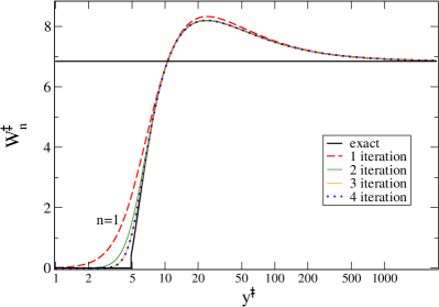
Figure 2: Log-plots of the iterative $W^{\ddagger}_{n}$, $n=1\ -\ 4$ and “exact” numerical solutions (thick solid line) for trace of the Reynolds tensor in sum-MM with constants, taken from Eq. (33). Plots for $W^{\ddagger}_{3}$ and $W^{\ddagger}_{4}$ coincide within the line width.

III Analysis of the numerical and experimental data and comparison with the model prediction

In this Section we analyze and compare the predictions of the minimal models to results of experiments and comprehensive direct numerical simulations of high Re channel flows. We refer to results that were made available in the public domain by R. G. Moser, J. Kim, and N. N. Mansour DNS , to Large-Eddy-Simulation performed by C. Casciola LES , and to recent laboratory experiments in a vertical water tunnel by A. Angrawal, L. Djenidi and R.A. Antonia Exp . The choice of the outer layer parameters $b_{ij}$ and $\widetilde{b}_{ij}$ is based on our analysis of the anisotropy in the log-low region, presented in Sec. III.1. The relation between the viscous layer parameters $a$ vs. $\widetilde{a}$ is based on the comparison between the DNS and the model mean velocity profiles, presented in Sec. III.2. The final choice of $a$ and $\widetilde{a}$ is motivated by the DNS data for the kinetic profile which is compared with the model prediction in Sec. III.3. Section III.4 is devoted to the comparison of the model results with the DNS profiles of the Reynolds stress $W^{\ddagger}_{xy}$ and partial kinetic energies $W^{\ddagger}_{xx}$, $W^{\ddagger}_{yy}$, $W^{\ddagger}_{zz}$.

III.1 Anisotropy of the log-layer: Relative partial kinetic energies $R_{xx}$, $R_{yy}$, $R_{zz}$ in the outer layer

The anisotropy of turbulent boundary layer can be characterized by the dimensionless ratios

$$R_{ii}(y^{+})\equiv\frac{W_{ii}(y^{+})}{W(y^{+})}=\frac{W^{+}_{ii}(y^{+})}{W^{+}(y^{+})}\,.$$ (46)

This anisotropy plays an important role in various phenomena and was a subject of experimental and theoretical concern for many decades, see, e.g. MY ; 00Pope . Nevertheless, up to now the dispersion of results on the subject appears quite large. There is a widely spread opinion, based on atmospheric measurements, that the wall-normal turbulent fluctuations $W_{yy}$ are much smaller than the other ones. For example, Monin and Yaglom MY reported that for a neutrally stratified log-boundary layer $R_{xx}=54\%$, $R_{yy}=6\%$ and $R_{zz}=40\%$. This contradicts recent DNS results for Re_λ=590 which are available in Ref. DNS , as shown in Fig. 3. Note that there is a region about $100<y^{+}<\frac{2}{3}\mbox{Re}_{\lambda}$ where the plots of $R_{ii}(y^{+})$ are nearly horizontal, as expected in the log-law region. From these plots we can conclude that is this region $R_{xx}\approx 53\%$ which is close to the value $54\%$, stated in MY . Nevertheless, the DNS data for $R_{yy}$ and $\mathcal{R}_{zz}$ are completely different. From Fig. 3 one gets $\mathcal{R}_{yy}\approx 22\%$ and $\mathcal{R}_{zz}\approx 27\%$. Thus $\mathcal{R}_{yy}$ can be considered roughly equal to $\mathcal{R}_{zz}$. We should mention here that various models of turbulent boundary layers give $\mathcal{R}_{yy}=\mathcal{R}_{zz}$ in the asymptotic log-law region. We propose that the difference between $\mathcal{R}_{yy}$ and $\mathcal{R}_{zz}$ which is observed in Fig. 3 is due to the effect of the energy transfer. This effect practically vanishes in the asymptotic limit Re${}_{\lambda}\to\infty$, but is still present at values of Re_λ which are available in DNS DNS . Indeed, for both values of Re_λ shown in Fig. 3, $W_{yy}=W_{zz}$ in the center of the channel, where the energy flux vanishes by symmetry. Clearly, there is no energy flux also in space homogeneous cases, for example for a constant shear flow, in which, according to the model, one should expect $W_{yy}=W_{zz}$ in the entire space.

Our expectation that $W_{yy}=W_{zz}$, which is based on symmetry considerations, is confirmed by the Large Eddy Simulation (LES) of the constant shear flow LES . As one sees in Fig. 4 in this flow $\mathcal{R}_{xx}\approx 0.46$, while $W_{yy}\approx W_{zz}\approx 0.27$.

As stated, for sufficiently large values of Re_λ the energy transfer terms should almost vanish in the log-law region and, according to our model, one can expect in that region $W_{yy}=W_{zz}$ also in the channel flow. This viewpoint was confirmed in the aforementioned laboratory experiment  Exp in a vertical water channel with Re${}_{\lambda}=1000$, reproduced in Fig. 5. The experimental values of $\mathcal{R}_{xx}$, $\mathcal{R}_{yy}$ and $\mathcal{R}_{zz}$ in the log-law turbulent region are in the excellent quantitative agreement with the values $\mathcal{R}_{xx}=0.5$ and $\mathcal{R}_{yy}=\mathcal{R}_{zz}=0.25$ shown in Figs. 3 and 5 by horizontal dashed lines.

Table 1 summaries the DNS, LES and experimental values of the relative kinetic energies in comparison with the model expectation. The conclusion is that, in contradiction with the old and still wide spread viewpoint MY that the wall-normal turbulent activity is strongly suppressed, $\mathcal{R}_{yy}<0.1$, the turbulent kinetic energy in the log-law region is distributed in a very simple manner: the stream-wise component contains a half of total energy, $\mathcal{R}_{xx}=\frac{1}{2}$ and the rest is equally distributed between the wall-normal and span-wise components: $\mathcal{R}_{yy}=\mathcal{R}_{zz}=\frac{1}{4}$. As shown in Sec. II.1.4, this very simple energy distribution is predicted by the minimal model if one assumes that the characteristic nonlinear times scales in the energy transfer term and in the return-to-isotropy term are identical.

Thus anisotropy predicted by our minimal model agree reasonably accurately with those obtained from DNS, LES and vertical water channel. However, we must admit that all these are not yet the nature. Indeed DNS, LES and lab experiments, done at relatively modest Re_λ impose limits on the low-frequency intervals in the spectra of the streamwise and the transverse velocity components, because of side walls or periodic boundary conditions. In other words, it must not be ruled out that DNS, as well as lab experiments, cat off the largest-scale ejections, observed in the atmosphere in the form of coherent structures, which pump additional streamwise- and transverse-velocity energies into the log-layer. Be it as it may, we leave a detailed discussion of the above problem and geophysical applications of our theory for further work. At the present stage, following our strategy of ”pragmatic, task-dependent simplification”, we consider our minimal model as definitely relevant to flows in channels. Its extension to geophysical (atmospheric and oceanic) boundary layers needs further efforts.

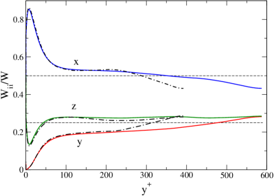
Figure 3: DNS profiles of the relative kinetic energies in the stream-wise, wall-normal and span-wise directions, $R_{xx}$, $R_{yy}$ and $R_{zz}$ respectively. Solid lines: Re${}_{\lambda}=590$, dot-dashed lines: Re${}_{\lambda}=395$. Horizontal dashed lines show levels 0.5 and 0.25.

Figure 4: Relative components of the Reynolds stress tensor $\widetilde{W}_{ii}$, Eq. (46), for for constant-shear flow. Results of the LES LES . Lines serve only to guide the eye.

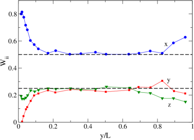
Figure 5: Experimental profiles of the relative kinetic energies $\mathcal{R}_{ii}$ in a vertical water channel with Re${}_{\lambda}=1000$ according to Ref. Exp . The solid lines serve to guide the eye. The dashed lines show the model prediction in the log-law region $\mathcal{R}_{xx}=0.5$ and $\mathcal{R}_{yy}=\mathcal{R}_{zz}=0.25$.

Table 1: Asymptotic values of the relative kinetic energies $\mathcal{R}_{ii}$ in the log-law region $y^{\ddagger}>200$ taken from DNS (Re${}_{\lambda}=395,\,590$) DNS , LES LES and experiment in a water channel with Re${}_{\lambda}=1000$ Exp . The last column presents the predictions of the minimal model.

${R_{ii,\infty}},\ \downarrow ii\downarrow$	DNS DNS	LES LES	Water channel Exp	Model
$xx~{}$	$\approx 0.53$	$\approx 0.46$	$0.50\pm 0.01$	0.50
$yy~{}$	$\approx 0.22$	$\approx 0.27$	$0.25\pm 0.02$	0.25
$zz~{}$	$\approx 0.27$	$\approx 0.27$	$0.25\pm 0.02$	0.25

III.2 Mean velocity profile in channel flows

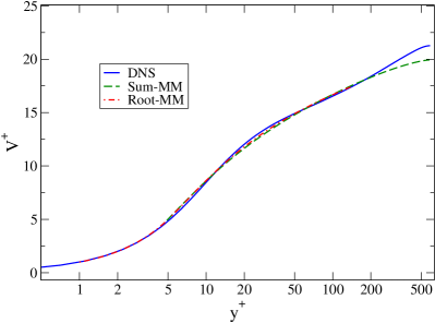
Figure 6: Mean velocity profiles $V^{+}(y^{+})$: The solid blue line – DNS data DNS for Re${}_{\tau}=590$, the dashed green line – analytical profile $V^{+}(y^{+})$ for the sum-MM, and dash-dotted red line for the root-MM using the parameters  Eq. (33). The relative deviation of the analytical predictions from the DNS data are about $1\%$, smaller for the root-MM than for the sum-MM.

To compute the mean velocity profile $V^{+}(y^{+})$ in our approach we need to connect first $S^{+}(y^{+})$ with $S^{\ddagger}(y^{\ddagger})$. According to the definitions (18) – (20):

$$S^{+}(y^{+})=\left(1-\frac{y^{+}}{\mbox{Re}_{\lambda}}\right)S^{\ddagger}\left(y^{+}\sqrt{1-\frac{y^{+}}{\mbox{Re}_{\lambda}}}\ \right)\,,$$ (47)

where

$$\mbox{Re}_{\lambda}\equiv L/\ell_{\tau}\,,$$ (48)

and $y^{+}>y_{\rm{vs}}$. For $y^{+}<\widehat{\bf{y}}_{\rm{vs}}$ we can take $S^{+}(y^{+})=1$ and integrate the resulting shear over the distance to the wall with no-slip boundary condition. The resulting profiles $V^{+}(y^{+})$ for Re${}_{\lambda}=590$ and the parameters (33) are shown in Fig. 6 as a dashed line for the sum-MM and as a dot-dashed line for the root-MM. The DNS profile of DNS for the same Re_λ is shown as a solid line. There is no significant difference (less than $1\%$) between these plots in the viscous sublayer, buffer and outer layers, where $y^{+}\lesssim 300$ i.e. in about 50% of the channel half-width $L^{+}=\mbox{Re}_{\lambda}=590$. This robustness of the mean velocity profile $V^{+}(y^{+})$ is a consequence of the fact that $V^{+}(y^{+})$ is an integral of the mean shear $S^{+}$ which is described very well both in the viscous and the outer layers.

Notice that our model does not describe the upward deviation from the log-low which is observed near the mid-channel (of about 5-6 units in $V^{+}$, independent on Reynolds number). We consider this minor disagreement as an acceptable price for the simplicity of the minimal model which neglects the energy transport term toward the centerline of the channel. This transport is the only reason for some turbulent activity near the centerline where both the Reynolds stress $W_{xy}$ and the mean shear $S$ vanish due to symmetry. Just at the center line the source term in our energy equation, $-2SW_{xy}$, is zero, and the missing energy transport term is felt.

The plots in Fig. 6 have a reasonably straight logarithmic region from $y^{+}\approx 20$ to $y^{+}\approx 200$. On the other hand, the Reynolds stress profile at the same Re${}_{\lambda}=590$ shown in Fig. 8, has no flat region at all. Such a flat region is expected in the true asymptotic regime of Re${}_{\lambda}\to\infty$, where $W^{+}=-1$. Therefore if one plots the model profiles $V^{+}$ at different Re_λ and fits them by log-linear profiles (32) one can get a Re_λ-dependence of the “effective” intercept in the von-Kármán log-law. We think that this explains, why measured value of the log-low intercept can depend on the Reynolds number and on the flow geometry (channel vs. pipe): both in DNS and in physical experiments one usually does not reach high enough values of Re_λ.

III.3 Profiles of the total kinetic energy density and the choice of the pair $a,\ \widetilde{a}$

The quality of the profiles $V^{+}(y^{+})$ calls for a bit more thinking. In fact, one find that the minimal model produces practically the same profiles $V^{+}(y^{+})$ not only for the parameters (35) but for a wide choice of the pairs $a,\ \widetilde{a}$, for example for $a=2$ and $\widetilde{a}=8.6$. Actually, for any $0\leq a\lesssim 4$ one can find a value of $\widetilde{a}$ that gives a mean velocity profile in good agreement with Fig. 6. In other words, in the $(a,\widetilde{a})$-plane there exist a long narrow corridor that produces a good quantitative description of $V^{+}(y^{+})$. Within this corridor there exists a line that provides a “best fit” of $V^{+}(y^{+})$, minimizing the mean square deviation $\delta V^{+}$

$$\delta V^{+}\equiv\sqrt{\left\langle[V_{\scriptscriptstyle\rm{MM}}^{+}(y^{+})-V_{\scriptscriptstyle\rm{DNS}}^{+}(y^{+})]^{2}\right\rangle}$$ (49)

of the model prediction $V_{\scriptscriptstyle\rm{MM}}^{+}(y^{+})$ from the DNS profile $V_{\scriptscriptstyle\rm{DNS}}^{+}(y^{+})$ in the inner region $y^{+}<140$. Some of the best pairs are given in Table 2 together with the corresponding values of $\delta V^{+}$. Table 2 also presents values of $y_{\rm{vs}}$ and $v_{*}$; recall: for $y^{\ddagger}<y_{\rm{vs}}\,,\ v^{\ddagger}=0$, for $y^{\ddagger}=y_{\rm{vs}}+0$ there is a jump of $v^{\ddagger}$ from zero to $v^{\ddagger}=v_{*}$. The most striking difference for different $(a,\ \widetilde{a})$ pairs is in the behavior of the Reynolds stress profiles $W^{\ddagger}(y^{\ddagger})$ that can be used to select the best values of these parameters.

Table 2: Optimal values of $\widetilde{a}$ for a given value of $a$, that $\delta V^{+}$ of Eq. (49). For optimal pairs $(a,\widetilde{a})$ in the sum and the root versions of the minimal model (denoted as $\sum$ and $\displaystyle\sqrt{~{}~{}}~{}$ correspondingly) we present the values $y_{\rm{vs}}$ of $y^{\ddagger}$, separating the viscous solution with $v^{\ddagger}=0$ from turbulent regime with $v_{*}\equiv v^{\ddagger}(y_{\rm{vs}}+0)$. The last two columns present the $y^{\ddagger}$ position, $y_{\rm{max}}$, of the maximum of the kinetic energy and the corresponding values of $W^{\ddagger}_{\rm{max}}\equiv W^{\ddagger}(y_{\rm{max}})$.

MM	$a$	$\widetilde{a}$	$\delta V^{\ddagger}$	$y_{\rm{vs}}$	$v_{*}$	$y_{\rm{max}}$	$W^{\ddagger}_{\rm{max}}$
$\sum$	0.1	10.4	0.29	1.5	0.017	21	8.33
$\sqrt{~{}~{}}$	0.1	12.0	0.25	1.1	0.008	18	8.32
$\sum$	0.25	10.9	0.25	2.4	0.061	22	8.48
$\sqrt{~{}~{}}$	0.25	12.1	0.25	2.1	0.016	19	8.36
$\sum$	0.5	11.1	0.25	3.4	0.159	22	8.47
$\sqrt{~{}~{}}$	0.5	12.6	0.17	3.4	0.247	19	8.50
$\sum$	1.0	10.7	0.22	4.8	0.401	24.6	8.24
$\sqrt{~{}~{}}$	1.0	12.9	0.15	4.9	0.234	19.2	8.59
$\sum$	1.5	9.7	0.20	5.7	0.600	27	7.76
$\sqrt{~{}~{}}$	1.5	12.9	0.16	4.8	0.743	19	8.58
$\sum$	2.0	8.6	0.19	6.4	0.783	27	7.26
$\sqrt{~{}~{}}$	2.0	11.8	0.17	6.7	0.743	20	8.13
$\sum$	4.0	2.9	0.21	7.2	0.630	$-$	$-$
$\sqrt{~{}~{}}$	4.0	6.3	0.46	8.5	1.04	$-$	$-$

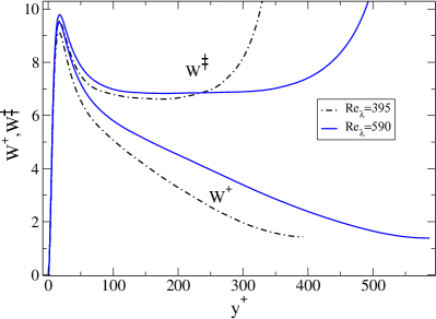
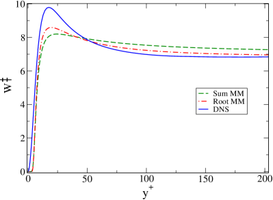
Figure 7: Upper panel: DNS profiles of the trace of the Reynolds-stress tensor (twice of the total kinetic energy densities) in two normalization, $W^{+}$ and $W^{\ddagger}$. Solid blue line: Re${}_{\tau}=590$ and dot-dashed black line – for Re${}_{\tau}=395$. Lower panel: Comparison of the DNS profile $W^{\ddagger}(y^{+})$ for Re${}_{\lambda}=590$ (blue solid line) with the results of the sum-MM (green dashed line) and the root-MM (red dot-dashed line) with constants Eq. (35).

Clearly, the minimal model with only 4 fit parameters cannot fit perfectly the profiles of all the physical quantities that can be measured. Therefore the actual values of $a$ and $\widetilde{a}$ should be determined with a choice of the characteristics of turbulent boundary layers that we desire to describe best. Foremost in any modeling should be the mean velocity profile which is of crucial importance in a wide variety of transport phenomena. Next we opt to fit well the profile of the kinetic energy density ([or, equivalently, the profile of the Reynolds stress tensor trace $W^{\ddagger}(y^{\ddagger})$] . Figure 7, upper panel, shows the DNS profiles of the trace of the Reynold-stress tensor $W^{+}(y^{+})$ for Re${}_{\lambda}=590$ (solid lower line) and Re${}_{\lambda}=395$ (dashed lower line). There are no plateau in these plots, meaning that these values of Re_λ are not large enough to have a true scale-invariant log-law region. Nevertheless, the plots of

$$W^{\ddagger}(y^{+})=(1-\frac{y^{+}}{{\rm Re}_{\lambda}})^{-1}W^{+}(y^{+})$$ (50)

(shown in the same upper panel of Fig. 7) display clear plateaus, according to the theoretical prediction for Re${}_{\lambda}\to\infty$. This means that the decay of $W^{+}(y^{+})$ is related to the decrease of the momentum flux $P(y)$ and that the dimensionless “ ^‡ ” variables, (20), that use the $y$-dependent value of the momentum flux $P(y)$ represent the asymptotic physics of the wall bounded turbulent flow, at lower values of Re_λ than the traditional “wall units” (18), which are based on the wall value of the momentum flux $P_{0}$.

To compare the model prediction with simulational results we have to relate $W^{\ddagger}_{ij}(y^{\ddagger})$ with $W^{+}_{ij}(y^{+})$ in channel flows. According to Eqs. (18) – (20):

$$W_{ij}^{+}(y^{+})=\left(1-\frac{y^{+}}{\mbox{Re}_{\lambda}}\right)W^{\ddagger}_{ij}\left(y^{+}\sqrt{1-\frac{y^{+}}{\mbox{Re}_{\lambda}}}\ \right)\,,$$ (51)

and similar Eqs. for the its trace $W^{+}(y^{+})$. Figure 7 shows a peak of $W^{\ddagger}(y^{+})$, $W^{\ddagger}_{\rm{max}}\equiv W^{\ddagger}(y_{\rm{max}})\approx 9.8$ at $y^{+}=y_{\rm{max}}\approx 18$. As one sees from the Tabl. 2, the minimal model reproduces the peak in $W^{\ddagger}(y^{\ddagger})$ with an amplitude of about $8\div 8.6$ for $a\lesssim 2$. To be specific we choose $a=1$ in both versions of the minimal model, sum-MM and root-MM. With this choice we plot in Fig. 7, lower panel, both theoretical profiles, $W^{\ddagger}_{{}_{\sum}}(y^{+})$ and $W^{\ddagger}_{{}_{\sqrt{~{}}}}(y^{+})$, in comparison with the simulational profile $W^{\ddagger}_{\scriptscriptstyle\rm{DNS}}(y^{+})$. It appears that the root-MM is in better correspondence with the simulation than the sum-MM. However, for the sake of analytic calculations, the sum-MM is simpler. Therefore, again, the choice of the version of MM depends on what is more important for a particular application: calculational simplicity or accuracy of fit.

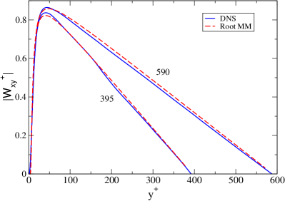
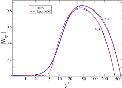
Figure 8: Comparison of the DNS Reynolds stress profiles $|W^{+}_{xy}|$ (blue solid lines) for the channel flow with Re${}_{\lambda}=395$ and $590$ with the root-MM profiles with constants (35)), red dashed lines. Upper panel: linear coordinates, lower panel: the same plots in the linear-log coordinates.

III.4 Profiles of the Reynolds stress tensor

In Fig. 8 we present (by solid lines) simulational profiles of the Reynolds stress $W^{+}_{xy}(y^{+})$ for Re${}_{\lambda}=395$ and Re${}_{\lambda}=590$ in comparison with the model predictions (dashed lines) for the root-MM. The upper panel shows the comparison in linear coordinates, the lower panel in linear-log coordinates, stressing the buffer layer region. In the model profiles we used the values of parameters (35), chosen to fit the simulational profiles for the mean velocity and the kinetic energy. In other words, in comparing the profiles of $W^{+}_{xy}(y^{+})$ in Fig. 8 no further fitting was exercised. Having this in mind, we consider the agreement as very encouraging. The only difference between the model predictions and the simulational profiles of $W^{+}_{xy}(y^{+})$ is in a steeper front of the model profiles for $y^{+}<20$. This is again because the model does not account for the energy transfer that can only flatten the front. As already mentioned, even for Re=590 the maximum value of the Reynolds stress does not reach it asymptotical value $|W^{+}_{xy}|=1$, as it should in the true log-law region. The corresponding comparison for the sum-MM looks very similar and is therefore not shown.

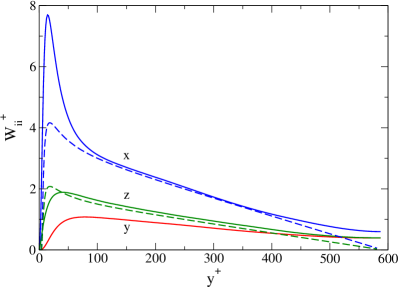
Figure 9: Comparison of the DNS (solid lines) and root-MM results (dashed lines) for partial kinetic energies profiles in the channel flow with Re${}_{\lambda}=590$. The model parameters are taken from (35).

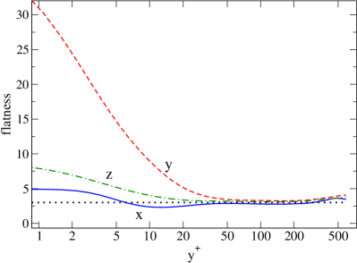
Figure 10: Profiles of the flatness of the $x$, $y$ and $z$ components of the turbulent velocity fluctuations, DNS data DNS for Re${}_{\tau}=590$. Horizontal dotted line shows Gaussian value for the flatness, equal to three.

Next, we present in Fig. 9 the simulational and root-MM profiles of the diagonal components of the Reynolds-stress tensor, $W^{+}_{ii}(y^{+})$ for the channel flow with Re${}_{\lambda}=590$. Solid lines present simulational profiles, dashed lines – the model profiles. The stream-wise and span-wise profiles, $W^{+}_{xx}(y^{+})$ and $W^{+}_{zz}(y^{+})$, are in good agreement in the most of the channel, $70<y^{+}<470$, while for the wall-normal component, the model profile $W^{+}_{yy}(y^{+})=W^{+}_{zz}(y^{+})$ and differs from the simulational one. The model also predicts semi-quantitatively increase in the streamwise part of the kinetic energy and the decrease in the span-wise and wall-normal components in the buffer layer which is observed in simulations. The physical reason of this is simple: as is well known, the energy from the mean flow is transferred only to the stream-wise component of the turbulent fluctuations. Accordingly, in the model one sees the energy production term ($-2SW_{xy}$) only in the RHS of equation for $W_{xx}$. The energy redistributes between other components due to “return-to-isotropy” term $I_{ij}$, Eq. (14b) with the isotropisation frequency $\propto 1/y$. The relative importance of $I_{ij}$ (in comparison with the energy relaxation term) decreases toward the wall due to the viscous contribution $\propto 1/y^{2}$. Accordingly, near the wall only a small part of the kinetic energy can be transferred from the streamwise to the wall-normal and the span-wise components of the velocity during the relaxation time (that $\propto 1/\Gamma$). Also, the model describes well the part (about $50\%$ in the outer layer) of the total kinetic energy that contains the streamwise components.

In the core of the flow ($y^{+}>450$) the model gives smaller values of all the components $W^{+}_{ii}$, as compared to simulations and experiments. This is again because the model neglects the energy transfer toward the centerline of the channel, where the energy input into turbulence, $-2SW_{xy}$, disappears due to the symmetry reason.

Also, there is a quantitative disagreement between the model and the simulations in the buffer layer. One can relate this with the fact that the model neglects the energy flux toward the wall, which plays a considerable role in the energy balance. The minimal models are local in space, but this effect can be effectively accounted for by an appropriate choice of the dissipation constants, taking $a_{yy}>a_{xx}=a_{zz}$. We do not propose to take this route; in the buffer layer the turbulent flow is strongly affected by highly intermittent events (coherent structures) connected with the near-wall instabilities of the laminal sub-layer. This is confirmed by the very large values of the flatness (above 30), as shown in Fig. 10. Only for $y^{+}>50$ the flatness reaches the Gaussian value of 3 and one can successfully utilize various lower-order closure model for describing wall bounded flows.

IV Summary: strength and limitations of the minimal model

The minimal model as formulated in this paper is a version of the algebraic Reynolds stress models. Its aim is to describe, for wall bounded turbulent flows, the profile of mean flow and the statistics of turbulence on the level of simultaneous, one-point, second-order velocity correlation functions, i.e. the entries of the Reynolds-stress tensor $W_{ij}$. The model was developed explicitly for plain geometry, including a wide variety of turbulent flows, like channel and plain Couette flows, to some extent fluid flows over inclined planes under gravity (modelling river flows), atmospheric turbulent boundary layers over flat planes and, in the limit of large Reynolds numbers, many other turbulent flows, including pipe, circular Couette flows, etc.

In developing a simple model one needs to decide what are the physically important aspects of the flow statistics, those which determine the mean-flow and the turbulent transport phenomena. The choice of the Reynolds-stress approach was dictated by the decision to emphasize the accurate description of $V(y)$- and $W_{ij}(y)$- profiles. The main criteria in constructing the model were simplicity, physical transparency, and maximal analytical tractability of the resulting model. That is why we took liberty to ignore the spatial energy flux, and, thanks to the plain geometry, to estimate the spatial derivatives and the outer scale of turbulence using the distance to the wall $y$. The same motivations led to choosing the simplest linear Rotta approximation of the “Return to isotropy term” 51Rot and the simplest dimensional form of the nonlinear term for energy flux down the scales, also in agreement with  51Rot .

By proper parametrization the number of fit parameters was reduced from twelve to four. Two of these, $a$ and $\widetilde{a}$ are responsible for the viscous dissipation of the diagonal, $W_{ii}$ , and the off-diagonal, $W_{xy}$, components of the Reynolds-stress tensor. The other two parameters - $b$ and $\widetilde{b}$ – control the nonlinear relaxation of $W_{ii}$ and $W_{xy}$. It appears that one cannot decrease the number of fit parameters further with impunity. The outer layer parameters $b=0.256$ and $\widetilde{b}=0.500$ where chosen to describe the observed constant values of von-Kármán in the log-law (32) and the asymptotic level of the density of kinetic energy. The viscous layer parameters were chosen to describe the observed values of the intersection $C$ in the von-Kármán log-law (32) and the peak of the kinetic energy in the buffer sub-layer. The resulting set of 5 equations for the mean shear $S(y)$, Reynolds stress $W_{xy}$ and $W_{xx}$, $W_{yy}$, $W_{zz}$ with just four fit parameters is referred to as the minimal model.

As demonstrated in Sec. III the minimal model with the given set (35) of four parameters describes five functions:

• the mean velocity profile $V(y)$ is describe with accuracy of $\simeq 1\%$ – almost throughout the channel (except of small velocity defect in the core of the flow), cf. Fig. 6;

• the Reynolds stress profile $W_{xy}(y)$ is also described with accuracy of few percents (except in the viscous layer $y^{+}<5$ in which $W_{xy}$ does not contribute to the mechanical balance), cf. Fig. 8;

• the total kinetic energy profile $\frac{1}{2}W(y)$ is reproduced with reasonable (semi-quantitative) accuracy, including the position and width of its peak in the buffer sub-layer, cf. Fig. 7;

• The profiles of the partial kinetic energies, $\frac{1}{2}W_{xx}(y)$, $\frac{1}{2}W_{yy}(y)$ and $\frac{1}{2}W_{zz}(y)$, are reproduced, see Fig. 9, including the simple $\,\frac{1}{2}\,$-$\,\frac{1}{4}\,$-$\,\frac{1}{4}\,$ distribution in the asymptotic outer region. This distribution is supported by recent experimental, DNS and LES data, as shown in Figs. 3, 4, and 5.

We consider all this as a good support of the minimal model; too much data is being reproduced to be an accident. It appears that the minimal model takes into account the essential physics almost throughout the channel flow.

On the other hand, one should accept that such a simple model cannot pretend to describe all the aspects of the turbulent statistics in wall bounded flows. For example, the minimal model ignores the quasi-two dimensional character of turbulence and the existence of coherent structures in the very vicinity of the wall. The minimal model does not attempt to take into account many-point and high-order turbulent statistics, including three-point velocity correlation functions and pressure-velocity correlations, responsible for the spatial energy flux and for the isotropization of turbulence. Finally, our choice of dissipation term definitely contradicts to the near-wall expansion, (and see Sec. 11.7.4 of  00Pope ), in disagreement with various known improvements of  51Rot . We propose that all this is a reasonable price for the simplicity and transparency of the minimal model, which is constructed with emphasis on the fundamental characteristics $V(y)$ and $W_{ij}(y)$ which are crucial for most applications.

We trust that a proper generalization of the minimal model will be found useful in the futures in studies of more complicated turbulent flows, laden with heavy particles, bubbles, etc.

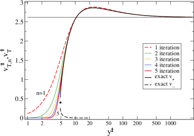
Figure 11: Log-plots of functions $v^{\ddagger}_{\infty}\approx 2.62$ (horizontal straight line), and profiles $v^{\ddagger}_{n}(y^{\ddagger})$ in the sum-MM for $n=1$ (the dashed line), $2,\,3,\,4,\,5$ together with the “exact” (numerical) solutions of Eq. (39a), $v^{\ddagger}_{+}(y^{\ddagger})$ (the thick solid line) and $v^{\ddagger}_{-}(y^{\ddagger})$ (dot-dashed line). Constants are given by (35). For this choice the critical point (designated as a black circle) corresponds to $v^{\ddagger}_{*}\approx 0.4$ at $y^{\ddagger}_{\rm{vs}}\approx 4.9$.

Appendix A Validation of the iterative procedure

To see, how the iterative procedure described in Sec. II.2.2 works, we plotted in Fig. 11 iterative profiles of the turbulent velocity $v^{\ddagger}_{n}(y^{\ddagger})$ for $n=1,\dots 5$ together with the (numerical) solutions of Eq. (39a), $v^{\ddagger}_{+}(y^{\ddagger})$ (the thick solid line) and $v^{\ddagger}_{-}(y^{\ddagger})$ (dot-dashed curve). The horizontal straight line presents the asymptotic value $v^{\ddagger}_{\infty}$. The critical point $\{v^{\ddagger}_{*},\,y^{\ddagger}_{\rm{vs}}\}$ is shown by a black circle. Our analysis shows (and see also Fig. 11), that already the simple Eq. (44a) gives the relative accuracy (with respect to $v^{\ddagger}_{\infty}$) better than 1% for $y^{\ddagger}>30$. The second iteration works with this accuracy in wider region $y^{\ddagger}>10$, the third iteration gives 1% accuracy for $y^{\ddagger}\approx 5$, which is about the critical value $y^{\ddagger}_{\rm{vs}}\approx 4.8$. Unexpectedly, the approximate solutions work even below the $y^{\ddagger}_{\rm{vs}}$, where exact solution is $v^{\ddagger}=0$. One observes with increasing $n$ the widening of the region, in which $v^{\ddagger}_{n}$ practically indistinguishable from zero. The overall conclusion from these observations is that already the fist few iterations give a very good accuracy for all practical purposes, and very often one can use only the first or the second iteration.

References

- (1) A. S. Monin and A. M. Yaglom, Statistical Fluid Mechanics (MIT, 1979, vol. 1 chapter 3).
- (2) U. Frisch, Turbulence: The Legasy of A.N. Kolmogorov (Cambridge University Press, Cambridge, 1995).
- (3) R.H. Kraichnan, Phys. Fliuds 9, 1728 (1966).
- (4) V. Yakhot and S. Orszag, Phys. Rev. Letts. 57, 1722 (1986).
- (5) Pope, S. B.: 2000, Turbulent Flows, University Press, Cambridge.
- (6) V. S. L’vov, A. Pomyalov, I. Procaccia and V. Tiberkevich, Phys. Rev. Lett., 92 244503, (2004).
- (7) E. De Angelis, C. Casciola, V. S. L’vov, A. Pomyalov, I. Procaccia and V. Tiberkevich, Phys. Rev. E, 70, 055301 (2004).
- (8) R. Benzi, V. S. L’vov, I. Procaccia and V. Tiberkevich, EuroPhysics Letters. 68, 825 (2004), DOI: 10.1209/epl/i2004-10282-6.
- (9) V S. L’vov, A. Pomyalov, I. Procaccia and V. Tiberkevich, Phys. Rev. E 71, 016305 (2005).
- (10) V. S. L’vov, A. Pomyalov, I. Procaccia and V. Tiberkevich, , Phys. Rev. Letts., 94, 174502, (2005). DOI:10.1103/PhysRevLett.94.174502.
- (11) R. Benzi, E. de Angelis, V. S. L’vov, I. Procaccia and V. Tiberkevich, “Maximum Drag Reduction Asymptotes and the Cross-Over to the Newtonian plug”, JFM, in press. Also: nlin.CD/0405033.
- (12) V. S. L’vov, A. Pomyalov and V. Tiberkevich, Simple analytical model for entire turbulent boundary layer over flat plane, Environmental Fluid Mechanics, in press. Also:nlin.CD/0404010
- (13) R. Benzi, E. S.C. Ching, T. S. Lo, V. S. L’vov, and I. Procaccia, Additive Equivalence in Turbulent Drag Reduction by Flexible and Rodlike Polymers, Phys. Rev. E., in press. Also:nlin.CD/0501027
- (14) R. Benzi, E. deAngelis, V. S. L’vov and I. Procaccia, Identification and Calculation of the Universal Maximum Drag Reduction Asymptote by Polymers in Wall Bounded Turbulence, Phys. Rev. Letts., submitted Also: nlin.CD/0505010
- (15) Moser, R. G., Kim, J., and Mansour, N. N.: 1999, Direct numerical simulation of turbulent channel flow up to , Phys. Fluids 11, 943; DNS data at http://www.tam.uiuc.edu/Faculty/Moser/channel.
- (16) C.M. Casciola, private communication, (2005)
- (17) A. Agrawal, L. Djenidi and R.A. Antonia, “Evolution of the anisotropy over a flat plane with suction”, 12th International symposium on application of the laser technology to fluid mechanics, Lisbon, Portugal, July 2004. Available at URL http://in3.dem.ist.utl.pt/lxlaser2004/pdf/paper_28_1.pdf
- (18) Zagarola, M. V. and Smits, A. J: 1997, Scaling of the Mean Velocity Profile for Turbulent Pipe Flow, Phys. Rev. Lett. 78, 239.
- (19) J.C. Rotta Z. Phys., 129, 547 (1951).