Casorati Determinant Form of Dark Soliton Solutions of the Discrete Nonlinear Schrödinger Equation

Abstract

It is shown that the $N$-dark soliton solutions of the integrable discrete nonlinear Schrödinger (IDNLS) equation are given in terms of the Casorati determinant. The conditions for reduction, complex conjugacy and regularity for the Casorati determinant solution are also given explicitly. The relationship between the IDNLS and the relativistic Toda lattice is discussed.

1 Introduction

The nonlinear Schrödinger (NLS) equation,

$${\rm i}\psi_{t}=\psi_{xx}+\alpha|\psi|^{2}\psi\,,$$ (1)

is one of most important soliton equations in mathematics and physics. The study of discrete analogues of the NLS equation has received considerable attention recently from both physical and mathematical point of view. [1, 2] The integrable discrete nonlinear Schrödinger (IDNLS) equation is given by

$${\rm i}\frac{d\psi_{n}}{dt}=\psi_{n+1}+\psi_{n-1}+\alpha|\psi_{n}|^{2}(\psi_{n+1}+\psi_{n-1})\,.$$ (2)

The IDNLS equation was originally derived by Ablowitz and Ladik using the Lax formulation. [3, 4, 1] Thus the IDNLS equation is often called the Ablowitz-Ladik lattice.

The IDNLS equation can be bilinearized into

$$D_{t}G_{n}\cdot F_{n}=G_{n+1}F_{n-1}-F_{n+1}G_{n-1}\,,$$ (3)

$$F_{n}^{2}+\alpha G_{n}G_{n}^{*}=F_{n+1}F_{n-1}\,,$$ (4)

through the dependent variable transformation $\psi_{n}=({\rm i})^{n}G_{n}/F_{n}$ where $F_{n}$ is a real function, $G_{n}$ is a complex function and $G_{n}^{*}$ is its complex conjugate. The Hirota D-operator $D_{t}$ is defined by

$$D_{t}^{n}f\cdot g=\left(\partial_{t}-\partial_{t^{\prime}}\right)^{n}f(t)g(t^{\prime})|_{t^{\prime}=t}\,\,.$$

With this bilinear forms the IDNLS equation in the case of $\alpha=1$ can be solved by the Hirota bilinear method, i.e. $N$-bright soliton solutions are obtained [5, 6, 7, 8, 9, 10].

It is well known that the NLS equation with defocusing parameter ($\alpha<0$) has dark soliton solutions. It is easily confirmed that there is a stationary dark soliton solution

$$\psi_{n}=\exp(-2{\rm i}t\,{\rm sech}^{2}(k))\frac{\tanh(k)}{\sqrt{-\alpha}}\tanh(kn)$$ (5)

by the direct substitution of an ansatz of stationary solution into eq.(2). Understanding various properties of dark solitons in discrete lattices is important from physical point of view [11, 12, 13]. There are analytical results of the IDNLS equation under non-vanishing boundary condition using the perturbative Hirota method by Narita [14] and inverse scattering theory by Vekslerchik and Konotop [15]. However, the detailed anayisis of the solution and understanding the role of a lattice space parameter in the $N$-dark soliton solutions are missing in their results. In ref.Vekslerchik2, a determinant expression of dark soliton solutions is given, however for their boundary condition there is no carrier wave of the dark soliton. Besides this is a Grammian type determinant solution. The Casorati determinant solution which is well-known in discrete integrable systems is missing.

The relationship between the IDNLS and relativistic Toda lattice (RTL) equation was also pointed out by several authors [16, 17, 10]. An interesting open problem was given in conclusion in ref.Sadakane: The 2-component Casorati determinant solution of the IDNLS equation and RTL equation in ref.Sadakane is different from the single-component Casorati determinant solution of the RTL equation which was derived in ref.OKMS. Is there any relationship between the 2-component Casorati determinant solution and single-component Casorati determinant solution?

Our goal in this paper is to construct Casorati determinant form of $N$-dark soliton solutions with a lattice space parameter, analyze the detail of behaviour of $N$-dark soliton solutions and give an answer of the above open problem. In this article, we give an explicit formula of the dark soliton solutions. It is known that the dark soliton solutions for NLS are written in terms of Wronski determinants. We show that the solution for IDNLS is given in the Casorati determinant form which is a discrete analogue of the Wronskian.

This paper is organized as follows. In the next section, we discuss about the gauge transformation and bilinearization of IDNLS equation. In §3, we give bilinear identities for Casorati determinant both for the Bäcklund transformation of Toda lattice and the discrete 2-dimensional Toda lattice equation. In §4, we perform a reduction of the Casorati determinant which derives the bilinear form for IDNLS given in §2. The complex conjugate condition is considered in §5. In §6, we give examples of dark soliton solutions. We also clarify the relationship between the IDNLS and the relativistic Toda lattice in the final section.

2 Gauge Transformation of IDNLS

First of all, we should examine the transformation of IDNLS equation by gauge. Applying the gauge transformation,

$$\psi_{n}=u_{n}A\exp({\rm i}(\theta n-\omega t)),$$

eq. (2) is transformed as

$${\rm i}\frac{du_{n}}{dt}=-\omega u_{n}+(1+\alpha A^{2}|u_{n}|^{2})(u_{n+1}\exp({\rm i}\theta)+u_{n-1}\exp(-{\rm i}\theta))\,,$$

thus we can scale $|\alpha|$ by using the amplitude $A$. To obtain the dark soliton solutions, we set $\alpha=-(a^{2}-1)/a^{2}$, $(a>1)$. We also scale $t$ by $t\to a^{2}t$, then the IDNLS eq. (2) can be bilinearized into

$$({\rm i}D_{t}+\omega)G_{n}\cdot F_{n}=G_{n+1}F_{n-1}\exp({\rm i}\theta)+G_{n-1}F_{n+1}\exp(-{\rm i}\theta)\,,$$ (6)

$$a^{2}F_{n}^{2}-(a^{2}-1)G_{n}G_{n}^{*}=F_{n+1}F_{n-1}\,,$$ (7)

through the dependent variable transformation,

$$\psi_{n}=\frac{G_{n}}{F_{n}}\exp({\rm i}(\theta n-\omega t)),$$

where $F_{n}$ is a real function, $G_{n}$ is a complex function and $G_{n}^{*}$ is its complex conjugate.

The above gauge factor $\exp({\rm i}(\theta n-\omega t))$ is nothing but the carrier wave of the dark soliton, and essentially $u_{n}=G_{n}/F_{n}$ gives the envelope of the soliton solution. In the context of NLS, in order to construct physical solutions, it is more convenient to consider the above bilinear form than the one in eqs. (3) and (4). Using the bilinear forms, eqs. (6) and (7), we present the Casorati determinant form of dark soliton solutions of the IDNLS equation. Instead of applying the Hirota bilinear method directly to eqs. (6) and (7), we rather start from the algebraic identities for Casorati determinant and derive the bilinear form of IDNLS equation by using the reduction technique.

3 Bilinear Identities for Casorati Determinant

3.1 Bäcklund transformation of Toda lattice

We have the bilinear forms for Bäcklund Transformation (BT) of Toda lattice (TL) equation,

$$(aD_{x}-1)\tau_{n+1}(k+1,l)\cdot\tau_{n}(k,l)+\tau_{n}(k+1,l)\tau_{n+1}(k,l)=0\,,$$ (8)

$$(bD_{y}-1)\tau_{n-1}(k,l+1)\cdot\tau_{n}(k,l)+\tau_{n}(k,l+1)\tau_{n-1}(k,l)=0\,,$$ (9)

where $a$ and $b$ are constants.

Consider the following Casorati determinant solution,

$$\tau_{n}(k,l)=\left|\begin{array}[]{cccc}\varphi_{1}^{(n)}(k,l)&\varphi_{1}^{(n+1)}(k,l)&\cdots&\varphi_{1}^{(n+N-1)}(k,l)\cr\varphi_{2}^{(n)}(k,l)&\varphi_{2}^{(n+1)}(k,l)&\cdots&\varphi_{2}^{(n+N-1)}(k,l)\cr\vdots&\vdots&&\vdots\cr\varphi_{N}^{(n)}(k,l)&\varphi_{N}^{(n+1)}(k,l)&\cdots&\varphi_{N}^{(n+N-1)}(k,l)\cr\end{array}\right|,$$ (14)

where $\varphi_{i}^{(n)}$’s are arbitrary functions of two continuous independent variables, $x$ and $y$, and two discrete ones, $k$ and $l$, which satisfy the dispersion relations,

$$\partial_{x}\varphi_{i}^{(n)}(k,l)=\varphi_{i}^{(n+1)}(k,l),$$ (15)

$$\partial_{y}\varphi_{i}^{(n)}(k,l)=\varphi_{i}^{(n-1)}(k,l),$$ (16)

$$\Delta_{k}\varphi_{i}^{(n)}(k,l)=\varphi_{i}^{(n+1)}(k,l),$$ (17)

$$\Delta_{l}\varphi_{i}^{(n)}(k,l)=\varphi_{i}^{(n-1)}(k,l).$$ (18)

Here $\Delta_{k}$ and $\Delta_{l}$ are the backward difference operators with difference intervals $a$ and $b$, defined by

$$\Delta_{k}f(k,l)={f(k,l)-f(k-1,l)\over a},$$ (19)

$$\Delta_{l}f(k,l)={f(k,l)-f(k,l-1)\over b}.$$ (20)

For simplicity we introduce a convenient notation,

$$|{n_{1}}_{{}_{\scriptstyle k_{1},l_{1}}},{n_{2}}_{{}_{\scriptstyle k_{2},l_{2}}},\cdots,{n_{N}}_{{}_{\scriptstyle k_{N},l_{N}}}|=\left|\begin{matrix}\varphi_{1}^{(n_{1})}(k_{1},l_{1})&\varphi_{1}^{(n_{2})}(k_{2},l_{2})&\cdots&\varphi_{1}^{(n_{N})}(k_{N},l_{N})\cr\varphi_{2}^{(n_{1})}(k_{1},l_{1})&\varphi_{2}^{(n_{2})}(k_{2},l_{2})&\cdots&\varphi_{2}^{(n_{N})}(k_{N},l_{N})\cr\vdots&\vdots&&\vdots\cr\varphi_{N}^{(n_{1})}(k_{1},l_{1})&\varphi_{N}^{(n_{2})}(k_{2},l_{2})&\cdots&\varphi_{N}^{(n_{N})}(k_{N},l_{N})\cr\end{matrix}\right|.$$ (21)

In this notation, the solution for BT of TL, $\tau_{n}(k,l)$ in eq. (14), is rewritten as

$$\tau_{n}(k,l)=|n_{k,l},n+1_{k,l},\cdots,n+N-1_{k,l}|,$$ (22)

or suppressing the index $k$ and $l$, we simply write as

$$\tau_{n}(k,l)=|n,n+1,\cdots,n+N-1|.$$

We show that the above $\tau_{n}(k,l)$ actually satisfies the bilinear eqs. (8) and (9) by using the Laplace expansion technique[19, 20]. At first we investigate the difference formula for $\tau$. From eq. (17) we have

$$a\varphi_{i}^{(n+1)}(k+1,l)=\varphi_{i}^{(n)}(k+1,l)-\varphi_{i}^{(n)}(k,l).$$

Noticing this relation, we get

$$\tau_{n}(k+1,l) = |n_{k+1,l},n+1_{k+1,l},n+2_{k+1,l},\cdots,n+N-1_{k+1,l}|$$ (23)

$$= |n_{k,l},n+1_{k+1,l},n+2_{k+1,l},\cdots,n+N-1_{k+1,l}|$$ (24)

where we have subtracted the 2nd column multiplied by $$a$$ from the 1st column, (25)

$$= |n_{k,l},n+1_{k,l},n+2_{k+1,l},\cdots,n+N-1_{k+1,l}|$$

where we have subtracted the 3rd column multiplied by $$a$$ from the 2nd column, (26)

$$\cdots$$

$$= |n_{k,l},n+1_{k,l},\cdots,n+N-2_{k,l},n+N-1_{k+1,l}|,$$ (27)

that is,

$$\tau_{n}(k+1,l)=|n_{k,l},n+1_{k,l},\cdots,n+N-2_{k,l},n+N-1_{k+1,l}|.$$ (28)

Moreover in eq. (28), multiplying the $N$-th column by $a$ and adding the $(N-1)$-th column to the $N$-th column, we get

$$a\tau_{n}(k+1,l)=|n_{k,l},n+1_{k,l},\cdots,n+N-2_{k,l},n+N-2_{k+1,l}|.$$ (29)

Differentiating eq.(29) with $x$ and using eq.(15) we obtain

$$a\partial_{x}\tau_{n}(k+1,l)=|n_{k,l},n+1_{k,l},\cdots,n+N-3_{k,l},n+N-1_{k,l},n+N-2_{k+1,l}|$$

$$\quad\quad\quad\quad\quad\quad\quad+|n_{k,l},n+1_{k,l},\cdots,n+N-3_{k,l},n+N-2_{k,l},n+N-1_{k+1,l}|$$

$$\quad=|n_{k,l},n+1_{k,l},\cdots,n+N-3_{k,l},n+N-1_{k,l},n+N-2_{k+1,l}|+\tau_{n}(k+1,l)\,.$$ (30)

We have also

$$\partial_{x}\tau_{n}(k,l)=|n_{k,l},n+1_{k,l},\cdots,n+N-2_{k,l},n+N_{k,l}|\,.$$ (31)

In short, we write

$$\tau_{n}(k+1,l)=|n,n+1,\cdots,n+N-2,n+N-1_{k+1}|\,,$$ (32)

$$a\tau_{n}(k+1,l)=|n,n+1,\cdots,n+N-2,n+N-2_{k+1}|\,,$$ (33)

$$(a\partial_{x}-1)\tau_{n}(k+1,l)=|n,n+1,\cdots,n+N-3,n+N-1,n+N-2_{k+1}|\,,$$ (34)

$$\partial_{x}\tau_{n}(k,l)=|n,n+1,\cdots,n+N-2,n+N|\,.$$ (35)

Let us introduce an identity for $2N\times 2N$ determinant,

$$\left|\begin{array}[]{cccccccccccccc}n+1&\cdots&n+N-2&\hskip-5.0pt\vbox{ \vbox{ \vbox to4.0pt{ \vbox to4.0pt{ \vbox to1.0pt{} \nointerlineskip\vbox to2.0pt{\hbox to0.1pt{\vrule width=0.1pt,height=2.0pt}} \nointerlineskip\vbox to1.0pt{} }} \nointerlineskip\vbox to4.0pt{ \vbox to4.0pt{ \vbox to1.0pt{} \nointerlineskip\vbox to2.0pt{\hbox to0.1pt{\vrule width=0.1pt,height=2.0pt}} \nointerlineskip\vbox to1.0pt{} }} \nointerlineskip\vbox to4.0pt{ \vbox to4.0pt{ \vbox to1.0pt{} \nointerlineskip\vbox to2.0pt{\hbox to0.1pt{\vrule width=0.1pt,height=2.0pt}} \nointerlineskip\vbox to1.0pt{} }} \nointerlineskip\vbox to4.0pt{ \vbox to4.0pt{ \vbox to1.0pt{} \nointerlineskip\vbox to2.0pt{\hbox to0.1pt{\vrule width=0.1pt,height=2.0pt}} \nointerlineskip\vbox to1.0pt{} }} \nointerlineskip}}\hskip-5.0pt&n+N&\hskip-5.0pt\vbox{ \vbox{ \vbox to4.0pt{ \vbox to4.0pt{ \vbox to1.0pt{} \nointerlineskip\vbox to2.0pt{\hbox to0.1pt{\vrule width=0.1pt,height=2.0pt}} \nointerlineskip\vbox to1.0pt{} }} \nointerlineskip\vbox to4.0pt{ \vbox to4.0pt{ \vbox to1.0pt{} \nointerlineskip\vbox to2.0pt{\hbox to0.1pt{\vrule width=0.1pt,height=2.0pt}} \nointerlineskip\vbox to1.0pt{} }} \nointerlineskip\vbox to4.0pt{ \vbox to4.0pt{ \vbox to1.0pt{} \nointerlineskip\vbox to2.0pt{\hbox to0.1pt{\vrule width=0.1pt,height=2.0pt}} \nointerlineskip\vbox to1.0pt{} }} \nointerlineskip\vbox to4.0pt{ \vbox to4.0pt{ \vbox to1.0pt{} \nointerlineskip\vbox to2.0pt{\hbox to0.1pt{\vrule width=0.1pt,height=2.0pt}} \nointerlineskip\vbox to1.0pt{} }} \nointerlineskip}}\hskip-5.0pt&n+N-1_{k+1}&\hskip-5.0pt\vbox{ \vbox{ \vbox to4.0pt{ \vbox to4.0pt{ \vbox to1.0pt{} \nointerlineskip\vbox to2.0pt{\hbox to0.1pt{\vrule width=0.1pt,height=2.0pt}} \nointerlineskip\vbox to1.0pt{} }} \nointerlineskip\vbox to4.0pt{ \vbox to4.0pt{ \vbox to1.0pt{} \nointerlineskip\vbox to2.0pt{\hbox to0.1pt{\vrule width=0.1pt,height=2.0pt}} \nointerlineskip\vbox to1.0pt{} }} \nointerlineskip\vbox to4.0pt{ \vbox to4.0pt{ \vbox to1.0pt{} \nointerlineskip\vbox to2.0pt{\hbox to0.1pt{\vrule width=0.1pt,height=2.0pt}} \nointerlineskip\vbox to1.0pt{} }} \nointerlineskip\vbox to4.0pt{ \vbox to4.0pt{ \vbox to1.0pt{} \nointerlineskip\vbox to2.0pt{\hbox to0.1pt{\vrule width=0.1pt,height=2.0pt}} \nointerlineskip\vbox to1.0pt{} }} \nointerlineskip}}\hskip-5.0pt&&&\hbox{\O}&&\hskip-5.0pt\vbox{ \vbox{ \vbox to4.0pt{ \vbox to4.0pt{ \vbox to1.0pt{} \nointerlineskip\vbox to2.0pt{\hbox to0.1pt{\vrule width=0.1pt,height=2.0pt}} \nointerlineskip\vbox to1.0pt{} }} \nointerlineskip\vbox to4.0pt{ \vbox to4.0pt{ \vbox to1.0pt{} \nointerlineskip\vbox to2.0pt{\hbox to0.1pt{\vrule width=0.1pt,height=2.0pt}} \nointerlineskip\vbox to1.0pt{} }} \nointerlineskip\vbox to4.0pt{ \vbox to4.0pt{ \vbox to1.0pt{} \nointerlineskip\vbox to2.0pt{\hbox to0.1pt{\vrule width=0.1pt,height=2.0pt}} \nointerlineskip\vbox to1.0pt{} }} \nointerlineskip\vbox to4.0pt{ \vbox to4.0pt{ \vbox to1.0pt{} \nointerlineskip\vbox to2.0pt{\hbox to0.1pt{\vrule width=0.1pt,height=2.0pt}} \nointerlineskip\vbox to1.0pt{} }} \nointerlineskip}}\hskip-5.0pt&n+N-1\cr\cleaders\hbox{$\mkern 1.0mu\vbox{ \vbox to0.1pt{ \hbox to4.2pt{ \hfil\vrule width=2.0pt,height=0.1pt\hfil} }}\mkern 1.0mu$}\hfill\cr&\hbox{\O}&&\hskip-5.0pt\vbox{ \vbox{ \vbox to4.0pt{ \vbox to4.0pt{ \vbox to1.0pt{} \nointerlineskip\vbox to2.0pt{\hbox to0.1pt{\vrule width=0.1pt,height=2.0pt}} \nointerlineskip\vbox to1.0pt{} }} \nointerlineskip\vbox to4.0pt{ \vbox to4.0pt{ \vbox to1.0pt{} \nointerlineskip\vbox to2.0pt{\hbox to0.1pt{\vrule width=0.1pt,height=2.0pt}} \nointerlineskip\vbox to1.0pt{} }} \nointerlineskip\vbox to4.0pt{ \vbox to4.0pt{ \vbox to1.0pt{} \nointerlineskip\vbox to2.0pt{\hbox to0.1pt{\vrule width=0.1pt,height=2.0pt}} \nointerlineskip\vbox to1.0pt{} }} \nointerlineskip\vbox to4.0pt{ \vbox to4.0pt{ \vbox to1.0pt{} \nointerlineskip\vbox to2.0pt{\hbox to0.1pt{\vrule width=0.1pt,height=2.0pt}} \nointerlineskip\vbox to1.0pt{} }} \nointerlineskip}}\hskip-5.0pt&n+N&\hskip-5.0pt\vbox{ \vbox{ \vbox to4.0pt{ \vbox to4.0pt{ \vbox to1.0pt{} \nointerlineskip\vbox to2.0pt{\hbox to0.1pt{\vrule width=0.1pt,height=2.0pt}} \nointerlineskip\vbox to1.0pt{} }} \nointerlineskip\vbox to4.0pt{ \vbox to4.0pt{ \vbox to1.0pt{} \nointerlineskip\vbox to2.0pt{\hbox to0.1pt{\vrule width=0.1pt,height=2.0pt}} \nointerlineskip\vbox to1.0pt{} }} \nointerlineskip\vbox to4.0pt{ \vbox to4.0pt{ \vbox to1.0pt{} \nointerlineskip\vbox to2.0pt{\hbox to0.1pt{\vrule width=0.1pt,height=2.0pt}} \nointerlineskip\vbox to1.0pt{} }} \nointerlineskip\vbox to4.0pt{ \vbox to4.0pt{ \vbox to1.0pt{} \nointerlineskip\vbox to2.0pt{\hbox to0.1pt{\vrule width=0.1pt,height=2.0pt}} \nointerlineskip\vbox to1.0pt{} }} \nointerlineskip}}\hskip-5.0pt&n+N-1_{k+1}&\hskip-5.0pt\vbox{ \vbox{ \vbox to4.0pt{ \vbox to4.0pt{ \vbox to1.0pt{} \nointerlineskip\vbox to2.0pt{\hbox to0.1pt{\vrule width=0.1pt,height=2.0pt}} \nointerlineskip\vbox to1.0pt{} }} \nointerlineskip\vbox to4.0pt{ \vbox to4.0pt{ \vbox to1.0pt{} \nointerlineskip\vbox to2.0pt{\hbox to0.1pt{\vrule width=0.1pt,height=2.0pt}} \nointerlineskip\vbox to1.0pt{} }} \nointerlineskip\vbox to4.0pt{ \vbox to4.0pt{ \vbox to1.0pt{} \nointerlineskip\vbox to2.0pt{\hbox to0.1pt{\vrule width=0.1pt,height=2.0pt}} \nointerlineskip\vbox to1.0pt{} }} \nointerlineskip\vbox to4.0pt{ \vbox to4.0pt{ \vbox to1.0pt{} \nointerlineskip\vbox to2.0pt{\hbox to0.1pt{\vrule width=0.1pt,height=2.0pt}} \nointerlineskip\vbox to1.0pt{} }} \nointerlineskip}}\hskip-5.0pt&n&n+1&\cdots&n+N-2&\hskip-5.0pt\vbox{ \vbox{ \vbox to4.0pt{ \vbox to4.0pt{ \vbox to1.0pt{} \nointerlineskip\vbox to2.0pt{\hbox to0.1pt{\vrule width=0.1pt,height=2.0pt}} \nointerlineskip\vbox to1.0pt{} }} \nointerlineskip\vbox to4.0pt{ \vbox to4.0pt{ \vbox to1.0pt{} \nointerlineskip\vbox to2.0pt{\hbox to0.1pt{\vrule width=0.1pt,height=2.0pt}} \nointerlineskip\vbox to1.0pt{} }} \nointerlineskip\vbox to4.0pt{ \vbox to4.0pt{ \vbox to1.0pt{} \nointerlineskip\vbox to2.0pt{\hbox to0.1pt{\vrule width=0.1pt,height=2.0pt}} \nointerlineskip\vbox to1.0pt{} }} \nointerlineskip\vbox to4.0pt{ \vbox to4.0pt{ \vbox to1.0pt{} \nointerlineskip\vbox to2.0pt{\hbox to0.1pt{\vrule width=0.1pt,height=2.0pt}} \nointerlineskip\vbox to1.0pt{} }} \nointerlineskip}}\hskip-5.0pt&n+N-1\cr\end{array}\right|=0.$$

Applying the Laplace expansion to the left-hand side, we obtain the algebraic bilinear identity for determinants,

$$|n+1,\cdots,n+N-2,n+N,n+N-1_{k+1}|\times|n,n+1,\cdots,n+N-2,n+N-1|$$ (36)

$$- |n+1,\cdots,n+N-2,n+N-1,n+N-1_{k+1}|\times|n,n+1,\cdots,n+N-2,n+N|$$ (37)

$$- |n+1,\cdots,n+N-2,n+N,n+N-1|\times|n,n+1,\cdots,n+N-2,n+N-1_{k+1}|=0,$$ (38)

which is rewritten by using eqs. (32)-(35), into the differential bilinear equation,

$$(a\partial_{x}-1)\tau_{n+1}(k+1,l)\times\tau_{n}(k,l)-a\tau_{n+1}(k+1,l)\partial_{x}\tau_{n}(k,l)+\tau_{n+1}(k,l)\tau_{n}(k+1,l)=0.$$

This equation is equal to eq. (8).

Similarly we obtain

$$(b\partial_{y}-1)\tau_{n-1}(k,l+1)\times\tau_{n}(k,l)-b\tau_{n-1}(k,l+1)\partial_{y}\tau_{n}(k,l)+\tau_{n-1}(k,l)\tau_{n}(k,l+1)=0,$$

because the role of $y$, $l$ and $b$ is parallel to that of $x$, $k$ and $a$ except that the ordering of index $n$ is reversed. The above equation is equal to eq. (9). Hence we have proved that the Casorati determinant $\tau_{n}(k,l)$ in eq. (14) gives the solution for the BT of TL equation.

3.2 Discrete 2-dimensional Toda lattice

Using the Casoratian technique, we show that the bilinear form of discrete 2-dimensional Toda lattice (D2DTL) equation,

$$\tau_{n}(k+1,l+1)\tau_{n}(k,l)-\tau_{n}(k+1,l)\tau_{n}(k,l+1)$$ (39)

$$\quad=ab(\tau_{n}(k+1,l+1)\tau_{n}(k,l)-\tau_{n+1}(k+1,l)\tau_{n-1}(k,l+1)),$$ (40)

is also satisfied by the Casorati determinant.

Let us further examine the difference formula for the Casorati determinant $\tau_{n}$ in eq. (14). Similarly to eqs. (32) and (33), we have

$$\tau_{n}(k,l+1)=|n_{l+1},n+1,\cdots,n+N-2,n+N-1|,$$ (41)

$$b\tau_{n}(k,l+1)=|n+1_{l+1},n+1,\cdots,n+N-2,n+N-1|.$$ (42)

Thus $\tau_{n}(k+1,l+1)$ is given by

$$\tau_{n}(k+1,l+1)=|n_{k+1,l+1},n+1_{k+1},\cdots,n+N-2_{k+1},n+N-1_{k+1}|.$$ (43)

In the following we show that the shifts of index $k$ is condensed into only the right-most column of the determinant. From eqs. (17) and (18), $\varphi_{i}^{(n)}$ satisfies

$$\Delta_{l}\Delta_{k}\varphi_{i}^{(n)}=\varphi_{i}^{(n)},$$ (44)

that is,

$$\varphi_{i}^{(n)}(k,l)-\varphi_{i}^{(n)}(k-1,l)-\varphi_{i}^{(n)}(k,l-1)+\varphi_{i}^{(n)}(k-1,l-1)=ab\varphi_{i}^{(n)}(k,l),$$ (45)

which is rewritten as

$$(1-ab)\varphi_{i}^{(n)}(k+1,l+1) = \varphi_{i}^{(n)}(k,l+1)+\varphi_{i}^{(n)}(k+1,l)-\varphi_{i}^{(n)}(k,l)$$ (46)

$$= \varphi_{i}^{(n)}(k,l+1)+a\varphi_{i}^{(n+1)}(k+1,l).$$ (47)

Therefore multiplying the both hand sides of eq. (43) by $(1-ab)$ and rewriting the 1st column of the determinant by the use of eq. (47), we obtain

$$(1-ab)\tau_{n}(k+1,l+1)$$ (48)

$$= |n_{k,l+1},n+1_{k+1},\cdots,n+N-2_{k+1},n+N-1_{k+1}|$$ (49)

$$+ a|n+1_{k+1,l},n+1_{k+1},\cdots,n+N-2_{k+1},n+N-1_{k+1}|.$$ (50)

The second term in r.h.s. vanishes because its 1st and 2nd columns are the same. So we get

$$(1-ab)\tau_{n}(k+1,l+1)=|n_{l+1},n+1_{k+1},\cdots,n+N-2_{k+1},n+N-1_{k+1}|.$$ (51)

In the above determinant, by subtracting the $(j+1)$-th column multiplied by $a$ from the $j$-th column for $j=2,3,\cdots,N-1$, $\tau_{n}(k+1,l+1)$ is given by

$$(1-ab)\tau_{n}(k+1,l+1)=|n_{l+1},n+1,\cdots,n+N-2,n+N-1_{k+1}|.$$ (52)

As is shown, even if the two variables $k$ and $l$ are shifted, $\tau_{n}$ is also expressed in the determinant form whose columns are almost unchanged and only edges are varied. Thus we can use the Laplace expansion technique.

We consider an identity for $2N\times 2N$ determinant,

$$\left|\begin{array}[]{cccccccccccccc}n_{l+1}&\hskip-5.0pt\vbox{ \vbox{ \vbox to4.0pt{ \vbox to4.0pt{ \vbox to1.0pt{} \nointerlineskip\vbox to2.0pt{\hbox to0.1pt{\vrule width=0.1pt,height=2.0pt}} \nointerlineskip\vbox to1.0pt{} }} \nointerlineskip\vbox to4.0pt{ \vbox to4.0pt{ \vbox to1.0pt{} \nointerlineskip\vbox to2.0pt{\hbox to0.1pt{\vrule width=0.1pt,height=2.0pt}} \nointerlineskip\vbox to1.0pt{} }} \nointerlineskip\vbox to4.0pt{ \vbox to4.0pt{ \vbox to1.0pt{} \nointerlineskip\vbox to2.0pt{\hbox to0.1pt{\vrule width=0.1pt,height=2.0pt}} \nointerlineskip\vbox to1.0pt{} }} \nointerlineskip\vbox to4.0pt{ \vbox to4.0pt{ \vbox to1.0pt{} \nointerlineskip\vbox to2.0pt{\hbox to0.1pt{\vrule width=0.1pt,height=2.0pt}} \nointerlineskip\vbox to1.0pt{} }} \nointerlineskip}}\hskip-5.0pt&n+1&\cdots&n+N-2&n+N-1_{k+1}&\hskip-5.0pt\vbox{ \vbox{ \vbox to4.0pt{ \vbox to4.0pt{ \vbox to1.0pt{} \nointerlineskip\vbox to2.0pt{\hbox to0.1pt{\vrule width=0.1pt,height=2.0pt}} \nointerlineskip\vbox to1.0pt{} }} \nointerlineskip\vbox to4.0pt{ \vbox to4.0pt{ \vbox to1.0pt{} \nointerlineskip\vbox to2.0pt{\hbox to0.1pt{\vrule width=0.1pt,height=2.0pt}} \nointerlineskip\vbox to1.0pt{} }} \nointerlineskip\vbox to4.0pt{ \vbox to4.0pt{ \vbox to1.0pt{} \nointerlineskip\vbox to2.0pt{\hbox to0.1pt{\vrule width=0.1pt,height=2.0pt}} \nointerlineskip\vbox to1.0pt{} }} \nointerlineskip\vbox to4.0pt{ \vbox to4.0pt{ \vbox to1.0pt{} \nointerlineskip\vbox to2.0pt{\hbox to0.1pt{\vrule width=0.1pt,height=2.0pt}} \nointerlineskip\vbox to1.0pt{} }} \nointerlineskip}}\hskip-5.0pt&n&\hskip-5.0pt\vbox{ \vbox{ \vbox to4.0pt{ \vbox to4.0pt{ \vbox to1.0pt{} \nointerlineskip\vbox to2.0pt{\hbox to0.1pt{\vrule width=0.1pt,height=2.0pt}} \nointerlineskip\vbox to1.0pt{} }} \nointerlineskip\vbox to4.0pt{ \vbox to4.0pt{ \vbox to1.0pt{} \nointerlineskip\vbox to2.0pt{\hbox to0.1pt{\vrule width=0.1pt,height=2.0pt}} \nointerlineskip\vbox to1.0pt{} }} \nointerlineskip\vbox to4.0pt{ \vbox to4.0pt{ \vbox to1.0pt{} \nointerlineskip\vbox to2.0pt{\hbox to0.1pt{\vrule width=0.1pt,height=2.0pt}} \nointerlineskip\vbox to1.0pt{} }} \nointerlineskip\vbox to4.0pt{ \vbox to4.0pt{ \vbox to1.0pt{} \nointerlineskip\vbox to2.0pt{\hbox to0.1pt{\vrule width=0.1pt,height=2.0pt}} \nointerlineskip\vbox to1.0pt{} }} \nointerlineskip}}\hskip-5.0pt&&\hbox{\O}&&\hskip-5.0pt\vbox{ \vbox{ \vbox to4.0pt{ \vbox to4.0pt{ \vbox to1.0pt{} \nointerlineskip\vbox to2.0pt{\hbox to0.1pt{\vrule width=0.1pt,height=2.0pt}} \nointerlineskip\vbox to1.0pt{} }} \nointerlineskip\vbox to4.0pt{ \vbox to4.0pt{ \vbox to1.0pt{} \nointerlineskip\vbox to2.0pt{\hbox to0.1pt{\vrule width=0.1pt,height=2.0pt}} \nointerlineskip\vbox to1.0pt{} }} \nointerlineskip\vbox to4.0pt{ \vbox to4.0pt{ \vbox to1.0pt{} \nointerlineskip\vbox to2.0pt{\hbox to0.1pt{\vrule width=0.1pt,height=2.0pt}} \nointerlineskip\vbox to1.0pt{} }} \nointerlineskip\vbox to4.0pt{ \vbox to4.0pt{ \vbox to1.0pt{} \nointerlineskip\vbox to2.0pt{\hbox to0.1pt{\vrule width=0.1pt,height=2.0pt}} \nointerlineskip\vbox to1.0pt{} }} \nointerlineskip}}\hskip-5.0pt&n+N-1\cr\cleaders\hbox{$\mkern 1.0mu\vbox{ \vbox to0.1pt{ \hbox to4.2pt{ \hfil\vrule width=2.0pt,height=0.1pt\hfil} }}\mkern 1.0mu$}\hfill\cr n_{l+1}&\hskip-5.0pt\vbox{ \vbox{ \vbox to4.0pt{ \vbox to4.0pt{ \vbox to1.0pt{} \nointerlineskip\vbox to2.0pt{\hbox to0.1pt{\vrule width=0.1pt,height=2.0pt}} \nointerlineskip\vbox to1.0pt{} }} \nointerlineskip\vbox to4.0pt{ \vbox to4.0pt{ \vbox to1.0pt{} \nointerlineskip\vbox to2.0pt{\hbox to0.1pt{\vrule width=0.1pt,height=2.0pt}} \nointerlineskip\vbox to1.0pt{} }} \nointerlineskip\vbox to4.0pt{ \vbox to4.0pt{ \vbox to1.0pt{} \nointerlineskip\vbox to2.0pt{\hbox to0.1pt{\vrule width=0.1pt,height=2.0pt}} \nointerlineskip\vbox to1.0pt{} }} \nointerlineskip\vbox to4.0pt{ \vbox to4.0pt{ \vbox to1.0pt{} \nointerlineskip\vbox to2.0pt{\hbox to0.1pt{\vrule width=0.1pt,height=2.0pt}} \nointerlineskip\vbox to1.0pt{} }} \nointerlineskip}}\hskip-5.0pt&&\hbox{\O}&&&\hskip-5.0pt\vbox{ \vbox{ \vbox to4.0pt{ \vbox to4.0pt{ \vbox to1.0pt{} \nointerlineskip\vbox to2.0pt{\hbox to0.1pt{\vrule width=0.1pt,height=2.0pt}} \nointerlineskip\vbox to1.0pt{} }} \nointerlineskip\vbox to4.0pt{ \vbox to4.0pt{ \vbox to1.0pt{} \nointerlineskip\vbox to2.0pt{\hbox to0.1pt{\vrule width=0.1pt,height=2.0pt}} \nointerlineskip\vbox to1.0pt{} }} \nointerlineskip\vbox to4.0pt{ \vbox to4.0pt{ \vbox to1.0pt{} \nointerlineskip\vbox to2.0pt{\hbox to0.1pt{\vrule width=0.1pt,height=2.0pt}} \nointerlineskip\vbox to1.0pt{} }} \nointerlineskip\vbox to4.0pt{ \vbox to4.0pt{ \vbox to1.0pt{} \nointerlineskip\vbox to2.0pt{\hbox to0.1pt{\vrule width=0.1pt,height=2.0pt}} \nointerlineskip\vbox to1.0pt{} }} \nointerlineskip}}\hskip-5.0pt&n&\hskip-5.0pt\vbox{ \vbox{ \vbox to4.0pt{ \vbox to4.0pt{ \vbox to1.0pt{} \nointerlineskip\vbox to2.0pt{\hbox to0.1pt{\vrule width=0.1pt,height=2.0pt}} \nointerlineskip\vbox to1.0pt{} }} \nointerlineskip\vbox to4.0pt{ \vbox to4.0pt{ \vbox to1.0pt{} \nointerlineskip\vbox to2.0pt{\hbox to0.1pt{\vrule width=0.1pt,height=2.0pt}} \nointerlineskip\vbox to1.0pt{} }} \nointerlineskip\vbox to4.0pt{ \vbox to4.0pt{ \vbox to1.0pt{} \nointerlineskip\vbox to2.0pt{\hbox to0.1pt{\vrule width=0.1pt,height=2.0pt}} \nointerlineskip\vbox to1.0pt{} }} \nointerlineskip\vbox to4.0pt{ \vbox to4.0pt{ \vbox to1.0pt{} \nointerlineskip\vbox to2.0pt{\hbox to0.1pt{\vrule width=0.1pt,height=2.0pt}} \nointerlineskip\vbox to1.0pt{} }} \nointerlineskip}}\hskip-5.0pt&n+1&\cdots&n+N-2&\hskip-5.0pt\vbox{ \vbox{ \vbox to4.0pt{ \vbox to4.0pt{ \vbox to1.0pt{} \nointerlineskip\vbox to2.0pt{\hbox to0.1pt{\vrule width=0.1pt,height=2.0pt}} \nointerlineskip\vbox to1.0pt{} }} \nointerlineskip\vbox to4.0pt{ \vbox to4.0pt{ \vbox to1.0pt{} \nointerlineskip\vbox to2.0pt{\hbox to0.1pt{\vrule width=0.1pt,height=2.0pt}} \nointerlineskip\vbox to1.0pt{} }} \nointerlineskip\vbox to4.0pt{ \vbox to4.0pt{ \vbox to1.0pt{} \nointerlineskip\vbox to2.0pt{\hbox to0.1pt{\vrule width=0.1pt,height=2.0pt}} \nointerlineskip\vbox to1.0pt{} }} \nointerlineskip\vbox to4.0pt{ \vbox to4.0pt{ \vbox to1.0pt{} \nointerlineskip\vbox to2.0pt{\hbox to0.1pt{\vrule width=0.1pt,height=2.0pt}} \nointerlineskip\vbox to1.0pt{} }} \nointerlineskip}}\hskip-5.0pt&n+N-1\cr\end{array}\right|=0.$$

By the Laplace expansion, we have

$$|n_{l+1},n+1,\cdots,n+N-2,n+N-1_{k+1}|\times|n,n+1,\cdots,n+N-2,n+N-1|$$ (53)

$$- |n,n+1,\cdots,n+N-2,n+N-1_{k+1}|\times|n_{l+1},n+1,\cdots,n+N-2,n+N-1|$$ (54)

$$+ |n+1,\cdots,n+N-2,n+N-1,n+N-1_{k+1}|\times|n_{l+1},n,n+1,\cdots,n+N-2|=0.$$ (55)

Using eqs. (32), (33), (41), (42) and (52), we obtain from eq. (55),

$$(1-ab)\tau_{n}(k+1,l+1)\tau_{n}(k,l)-\tau_{n}(k+1,l)\tau_{n}(k,l+1)$$ (56)

$$+a\tau_{n+1}(k+1,l)b\tau_{n-1}(k,l+1)=0,$$ (57)

which recovers eq. (40). This completes the proof that the Casorati determinant is indeed the solution for D2DTL equation.

For example, we can take $\varphi_{i}^{(n)}$ as

$$\varphi_{i}^{(n)}(k,l)=p_{i}^{n}(1-ap_{i})^{-k}\left(1-b{1\over p_{i}}\right)^{-l}\exp(\xi_{i})+q_{i}^{n}(1-aq_{i})^{-k}\left(1-b{1\over q_{i}}\right)^{-l}\exp(\eta_{i}),$$ (58)

$$\xi_{i}=p_{i}x+{1\over p_{i}}y+\xi_{i0},\quad\eta_{i}=q_{i}x+{1\over q_{i}}y+\eta_{i0},$$

where $p_{i}$, $q_{i}$ and $\xi_{i0}$, $\eta_{i0}$ are arbitrary constants which correspond to the wave numbers and phase parameters of solitons, respectively. It can easily be seen that $\varphi_{i}^{(n)}$ in eq. (58) actually satisfies the dispersion relations, eqs. (15)-(18).

4 Reduction to IDNLS

In this section, we give the reduction technique in order to derive the IDNLS equation from the system of BT of TL and D2DTL. In eq. (58), we apply a condition for the wave numbers,

$$q_{i}=-p_{i}{1-b{1\over p_{i}}\over 1-ap_{i}}.$$ (59)

Then we get

$$p_{i}=-q_{i}{1-b{1\over q_{i}}\over 1-aq_{i}},$$ (60)

and thus

$$p_{i}^{2}{1-b{1\over p_{i}}\over 1-ap_{i}}=q_{i}^{2}{1-b{1\over q_{i}}\over 1-aq_{i}}.$$ (61)

On this condition, $\varphi_{i}^{(n)}$ in eq. (58) satisfies

$$\varphi_{i}^{(n+2)}(k+1,l-1)=p_{i}^{2}{1-b{1\over p_{i}}\over 1-ap_{i}}\varphi_{i}^{(n)}(k,l).$$ (62)

Hence we obtain

$$\tau_{n+2}(k+1,l-1)=\left(\prod_{i=1}^{N}p_{i}^{2}{1-b{1\over p_{i}}\over 1-ap_{i}}\right)\tau_{n}(k,l).$$ (63)

By using eq. (63), the bilinear forms for BT of TL and D2DTL, eqs. (8), (9) and (40), are rewritten as

$$(aD_{x}-1)\tau_{n+1}(k+1,l)\cdot\tau_{n}(k,l)+\tau_{n}(k+1,l)\tau_{n+1}(k,l)=0\,,$$ (64)

$$(bD_{y}-1)\tau_{n+1}(k+1,l)\cdot\tau_{n}(k,l)+\tau_{n+2}(k+1,l)\tau_{n-1}(k,l)=0\,,$$ (65)

$$\tau_{n+1}(k+1,l)\tau_{n-1}(k-1,l)-\tau_{n+1}(k,l)\tau_{n-1}(k,l)$$

$$\qquad=ab(\tau_{n+1}(k+1,l)\tau_{n-1}(k-1,l)-\tau_{n}(k,l)\tau_{n}(k,l)).$$ (66)

Here we may drop $l$-dependence, thus for simplicity we take $l=0$ hereafter. Equation (66) is nothing but the bilinear form of the discrete one-dimensional TL equation.

Let us substitute

$$x={\rm i}act,\qquad y={\rm i}bdt,$$ (67)

where $c$ and $d$ are constants. Then we have

$$-{\rm i}\partial_{t}=ac\partial_{x}+bd\partial_{y},$$ (68)

and from the bilinear eqs. (64) and (65), we get

$$(-{\rm i}D_{t}-c-d)\tau_{n+1}(k+1)\cdot\tau_{n}(k)+c\tau_{n}(k+1)\tau_{n+1}(k)+d\tau_{n+2}(k+1)\tau_{n-1}(k)=0\,.$$ (69)

The Casorati determinant solution of eqs. (69) and (66) (with $l=0$) is given by

$$\tau_{n}(k)=\left|\begin{matrix}\varphi_{1}^{(n)}(k)&\varphi_{1}^{(n+1)}(k)&\cdots&\varphi_{1}^{(n+N-1)}(k)\cr\varphi_{2}^{(n)}(k)&\varphi_{2}^{(n+1)}(k)&\cdots&\varphi_{2}^{(n+N-1)}(k)\cr\vdots&\vdots&&\vdots\cr\varphi_{N}^{(n)}(k)&\varphi_{N}^{(n+1)}(k)&\cdots&\varphi_{N}^{(n+N-1)}(k)\cr\end{matrix}\right|,$$

$$\varphi_{i}^{(n)}(k)=p_{i}^{n}(1-ap_{i})^{-k}\exp(\xi_{i})+q_{i}^{n}(1-aq_{i})^{-k}\exp(\eta_{i}),$$

$$\xi_{i}={\rm i}\left(acp_{i}+{bd\over p_{i}}\right)t+\xi_{i0},\qquad\eta_{i}={\rm i}\left(acq_{i}+{bd\over q_{i}}\right)t+\eta_{i0}.$$

Here $p_{i}$ and $q_{i}$ are related by eq. (59).

By defining

$$f_{n}=\tau_{n}(0),\qquad g_{n}=\tau_{n+1}(1),\qquad h_{n}=\tau_{n-1}(-1),$$ (70)

from eqs. (66) and (69), we obtain the bilinear form of IDNLS equation,

$$(-{\rm i}D_{t}-c-d)g_{n}\cdot f_{n}+dg_{n+1}f_{n-1}+cg_{n-1}f_{n+1}=0\,,$$ (71)

$$({\rm i}D_{t}-c-d)h_{n}\cdot f_{n}+ch_{n+1}f_{n-1}+dh_{n-1}f_{n+1}=0\,,$$ (72)

$$f_{n+1}f_{n-1}-f_{n}f_{n}=(ab-1)(f_{n}f_{n}-g_{n}h_{n})\,.$$ (73)

By using the dependent variable transformation,

$$u_{n}={g_{n}\over f_{n}},\qquad v_{n}={h_{n}\over f_{n}},$$

the above bilinear equations are transformed into

$${\rm i}{du_{n}\over dt}=-(c+d)u_{n}+(ab-(ab-1)u_{n}v_{n})(du_{n+1}+cu_{n-1})\,,$$ (74)

$$-{\rm i}{dv_{n}\over dt}=-(c+d)v_{n}+(ab-(ab-1)u_{n}v_{n})(cv_{n+1}+dv_{n-1})\,.$$ (75)

5 Complex Conjugate Condition

In order to take $v_{n}$ to be the complex conjugate of $u_{n}$, we need to restrict $f_{n}$ as real and $h_{n}$ as the complex conjugate of $g_{n}$ up to gauge freedom. Moreover to take $u_{n}$ to be regular (i.e., $u_{n}$ not to diverge for real $t$), we need $f_{n}\neq 0$ for real $t$. In this section, we give the conditions for the complex conjugacy and regularity for the Casorati determinant solution.

Firstly we take

$$b=a\,,$$

for simplicity, and next we take

$$a>1\,.$$

Then the conditions for complex conjugate are given as follows:

$$p_{i}=a+\sqrt{a^{2}-1}r_{i},\qquad|r_{i}|=1\,,$$ (76)

$$\exp(\eta_{i0})=\left(\prod_{{k=1\atop k\neq i}}^{N}{p_{i}-q_{k}\over q_{i}-q_{k}}\right)\exp(-\xi_{i0}^{*})\,,$$ (77)

$$d=c^{*}\,,$$ (78)

where $r_{i}$ is a complex parameter of absolute value $1$, and ^∗ means the complex conjugate. On the condition (76), eq. (59) turns to be

$$q_{i}={1\over p_{i}^{*}}\,,$$

and eqs. (77) and (78) gives

$$\exp(\eta_{i})=\left(\prod_{{k=1\atop k\neq i}}^{N}{p_{i}-q_{k}\over q_{i}-q_{k}}\right)\exp(-\xi_{i}^{*})\,,$$

for real $t$.

Now we summarize the final result of the Casorati determinant solution for IDNLS equation. The bilinear form of IDNLS equation is given as

$$(-{\rm i}D_{t}-c-c^{*})g_{n}\cdot f_{n}+c^{*}g_{n+1}f_{n-1}+cg_{n-1}f_{n+1}=0\,,$$ (79)

$$({\rm i}D_{t}-c-c^{*})h_{n}\cdot f_{n}+ch_{n+1}f_{n-1}+c^{*}h_{n-1}f_{n+1}=0\,,$$ (80)

$$f_{n+1}f_{n-1}-f_{n}f_{n}=(a^{2}-1)(f_{n}f_{n}-g_{n}h_{n})\,,$$ (81)

where $a>1$ and t is real. The Casorati determinant solution for the above bilinear equations is given as

$$f_{n}=\left|\begin{matrix}\varphi_{1}^{(n)}(0)&\varphi_{1}^{(n+1)}(0)&\cdots&\varphi_{1}^{(n+N-1)}(0)\cr\varphi_{2}^{(n)}(0)&\varphi_{2}^{(n+1)}(0)&\cdots&\varphi_{2}^{(n+N-1)}(0)\cr\vdots&\vdots&&\vdots\cr\varphi_{N}^{(n)}(0)&\varphi_{N}^{(n+1)}(0)&\cdots&\varphi_{N}^{(n+N-1)}(0)\cr\end{matrix}\right|,$$ (82)

$$g_{n}=\left|\begin{matrix}\varphi_{1}^{(n+1)}(1)&\varphi_{1}^{(n+2)}(1)&\cdots&\varphi_{1}^{(n+N)}(1)\cr\varphi_{2}^{(n+1)}(1)&\varphi_{2}^{(n+2)}(1)&\cdots&\varphi_{2}^{(n+N)}(1)\cr\vdots&\vdots&&\vdots\cr\varphi_{N}^{(n+1)}(1)&\varphi_{N}^{(n+2)}(1)&\cdots&\varphi_{N}^{(n+N)}(1)\cr\end{matrix}\right|,$$ (83)

$$h_{n}=\left|\begin{matrix}\varphi_{1}^{(n-1)}(-1)&\varphi_{1}^{(n)}(-1)&\cdots&\varphi_{1}^{(n+N-2)}(-1)\cr\varphi_{2}^{(n-1)}(-1)&\varphi_{2}^{(n)}(-1)&\cdots&\varphi_{2}^{(n+N-2)}(-1)\cr\vdots&\vdots&&\vdots\cr\varphi_{N}^{(n-1)}(-1)&\varphi_{N}^{(n)}(-1)&\cdots&\varphi_{N}^{(n+N-2)}(-1)\cr\end{matrix}\right|,$$ (84)

where

$$\varphi_{i}^{(n)}(k)=p_{i}^{n}(-\sqrt{a^{2}-1}p_{i}^{*}r_{i})^{-k}\exp(\xi_{i})+\left({1\over p_{i}^{*}}\right)^{n}\left({\sqrt{a^{2}-1}\over p_{i}^{*}r_{i}}\right)^{-k}\left(\prod_{{k=1\atop k\neq i}}^{N}{p_{k}^{*}p_{i}-1\over p_{k}^{*}/p_{i}^{*}-1}\right)\exp(-\xi_{i}^{*}),$$

$$\xi_{i}={\rm i}a\left(cp_{i}+{c^{*}\over p_{i}}\right)t+\xi_{i0},\qquad p_{i}=a+\sqrt{a^{2}-1}r_{i},\qquad|r_{i}|=1\,,$$

where $r_{i}$ is a complex parameter of absolute value $1$ and $\xi_{i0}$ is an arbitrary complex parameter. This Casorati determinant solution gives the $N$-dark soliton solution for IDNLS equation. $r_{i}$ and $\xi_{i0}$ parametrize the wave number and phase constant of $i$-th soliton, respectively.

After a straightforward and tedious calculation of expanding the determinants, $f_{n}$, $g_{n}$ and $h_{n}$ can be expressed in an explicit way as follows:

$$f_{n}=F_{n}{\cal G}\,,\qquad g_{n}=G_{n}{\cal G}{r_{1}r_{2}\cdots r_{N}\over(\sqrt{a^{2}-1})^{N}}\,,\qquad h_{n}=H_{n}{\cal G}{(\sqrt{a^{2}-1})^{N}\over r_{1}r_{2}\cdots r_{N}}\,,$$ (85)

where ${\cal G}$ is the gauge factor defined by

$${\cal G}=\prod_{N\geq i>j\geq 1}(q_{i}-q_{j})\prod_{i=1}^{N}q_{i}^{n}\exp(\eta_{i})\,,$$

and $F_{n}$, $G_{n}$ and $H_{n}$ are given as

$$F_{n}=\sum_{M=0}^{N}\ \sum_{1\leq i_{1}<i_{2}<\cdots<i_{M}\leq N}\left|\prod_{1\leq\mu<\nu\leq M}{p_{i_{\mu}}-p_{i_{\nu}}\over p_{i_{\mu}}p_{i_{\nu}}^{*}-1}\right|^{2}\prod_{\nu=1}^{M}|p_{i_{\nu}}|^{2n}{\rm e}^{\xi_{i_{\nu}}+\xi_{i_{\nu}}^{*}}\,,$$ (86)

$$G_{n}=\sum_{M=0}^{N}\ \sum_{1\leq i_{1}<i_{2}<\cdots<i_{M}\leq N}\left|\prod_{1\leq\mu<\nu\leq M}{p_{i_{\mu}}-p_{i_{\nu}}\over p_{i_{\mu}}p_{i_{\nu}}^{*}-1}\right|^{2}\prod_{\nu=1}^{M}\left(-{p_{i_{\nu}}\over p_{i_{\nu}}^{*}r_{i_{\nu}}^{2}}\right)|p_{i_{\nu}}|^{2n}{\rm e}^{\xi_{i_{\nu}}+\xi_{i_{\nu}}^{*}}\,,$$ (87)

$$H_{n}=\sum_{M=0}^{N}\ \sum_{1\leq i_{1}<i_{2}<\cdots<i_{M}\leq N}\left|\prod_{1\leq\mu<\nu\leq M}{p_{i_{\mu}}-p_{i_{\nu}}\over p_{i_{\mu}}p_{i_{\nu}}^{*}-1}\right|^{2}\prod_{\nu=1}^{M}\left(-{p_{i_{\nu}}^{*}r_{i_{\nu}}^{2}\over p_{i_{\nu}}}\right)|p_{i_{\nu}}|^{2n}{\rm e}^{\xi_{i_{\nu}}+\xi_{i_{\nu}}^{*}}\,.$$ (88)

A proof of the above expression is given in appendix BB. Now it is clear that $F_{n}$ is real and $H_{n}=G_{n}^{*}$, thus $v_{n}$ is the complex conjugate of $u_{n}$ up to multiplication factor. Moreover since $F_{n}>1$, the regularity of $u_{n}$ is also satisfied.

From the bilinear eqs. (79)-(81), and the gauge transformation (85), the above $F_{n}$ and $G_{n}$ satisfy the bilinear equations,

$$(-{\rm i}D_{t}-c-c^{*})G_{n}\cdot F_{n}+c^{*}G_{n+1}F_{n-1}+cG_{n-1}F_{n+1}=0\,,$$ (89)

$$F_{n+1}F_{n-1}-F_{n}F_{n}=(a^{2}-1)(F_{n}F_{n}-G_{n}G_{n}^{*})\,.$$ (90)

Let us take

$$c=\exp(-{\rm i}\theta),$$

where $\theta$ is a real parameter. By the variable transformation,

$$\psi_{n}={G_{n}\over F_{n}}\exp({\rm i}(\theta n-\omega t))\,,$$

that is,

$$\psi_{n}=u_{n}{(\sqrt{a^{2}-1})^{N}\over r_{1}r_{2}\cdots r_{N}}\exp({\rm i}(\theta n-\omega t))\,,$$

where

$$\omega=\exp({\rm i}\theta)+\exp(-{\rm i}\theta)=2\cos\theta\,,$$

we finally obtain the IDNLS equation,

$${{\rm i}\over a^{2}}\frac{d\psi_{n}}{dt}=\psi_{n+1}+\psi_{n-1}-\frac{a^{2}-1}{a^{2}}|\psi_{n}|^{2}(\psi_{n+1}+\psi_{n-1})\,.$$ (91)

Thus we have completed the proof that the $N$-dark soliton solutions for the IDNLS equation are given in terms of the Casorati determinant. Here we remark that a parameter $a$ is related to a lattice space parameter $\delta=1/a\,(<1)$. Using a lattice parameter $\delta$, we can rewrite the IDNLS equation (91) into

$${\rm i}\frac{d\psi_{n}}{dt}=\frac{\psi_{n+1}+\psi_{n-1}}{\delta^{2}}-\frac{1-\delta^{2}}{\delta^{2}}|\psi_{n}|^{2}(\psi_{n+1}+\psi_{n-1})\,.$$ (92)

We see that the IDNLS equation is defocusing whenever a lattice parameter $\delta$ is smaller than 1. When $\delta=1$, the IDNLS equation reduces to a linear equation. When $\delta>1$, i.e. $a<1$, the IDNLS equation is focusing. In this case, above single component Casorati determinant solution does not satisfy the conditions for complex conjugacy (unless we admit singular solutions). However, our Casorati determinant form can be extended into the case of the focusing IDNLS equation. This is corresponding to the homoclinic orbit solution of the IDNLS equation. The detail will be discussed in elsewhere.

6 Soliton Solutions

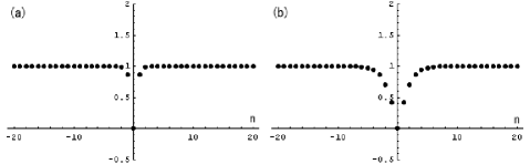
Figure 1: Plots of 1-dark soliton. The vertical axis is $|\psi_{n}|$. ((a) $a=2,r=\exp({\rm i}\pi),\theta=\pi$, (b) $a=1.1,r=\exp({\rm i}\pi),\theta=\pi$.)

In this section we give examples of dark soliton solutions for the IDNLS equation. By taking $N=1$ in eqs. (86) and (87), we get the 1-soliton solution for the IDNLS eq. (91),

$$\psi_{n}={G_{n}\over F_{n}}\exp({\rm i}(\theta n-2t\cos\theta))\,,$$

where $\theta$ is a real parameter and

$$F_{n}=1+|p_{1}|^{2n}\exp(\xi_{1}+\xi_{1}^{*})\,,\qquad G_{n}=1-{p_{1}\over p_{1}^{*}r_{1}^{2}}|p_{1}|^{2n}\exp(\xi_{1}+\xi_{1}^{*})\,,$$

where

$$\xi_{1}={\rm i}a\left({p_{1}\over\exp({\rm i}\theta)}+{\exp({\rm i}\theta)\over p_{1}}\right)t+\xi_{10},\qquad p_{1}=a+\sqrt{a^{2}-1}r_{1},\qquad|r_{1}|=1\,.$$

By rewriting as $p_{1}=p\exp({\rm i}\theta)$ and $r_{1}=r\exp({\rm i}\theta)$, we get a slightly simpler expression,

$$F_{n}=1+|p|^{2n}\exp(\xi+\xi^{*})\,,\qquad G_{n}=1-{p\over p^{*}r^{2}}|p|^{2n}\exp(\xi+\xi^{*})\,,$$

where

$$\xi={\rm i}a\left(p+{1\over p}\right)t+\xi_{0},\qquad p=a\exp(-{\rm i}\theta)+\sqrt{a^{2}-1}r,\qquad|r|=1\,.$$

Here $\arg(r)$ parametrizes the wave number of soliton, and $\Re(\xi_{0})$ gives the phase constant which parametrizes the position of soliton. Figure 1 shows a stationary 1-dark (black) soliton. When $a\,(>1)$ is getting closer to 1, the width of a dip is getting wider. Figures 2 and 3 show travelling 1-dark (gray and black) solitons.

Here we should comment about the difference of travelling velocity between black and gray solitons. In the continuous case, the NLS equation (1) is invariant under the gauge and Galilean transformations,

$$\psi(x,t)\to\psi(x-2kt,t)\exp({\rm i}(kx-k^{2}t)),$$

thus the travelling velocity of any solution can be shifted by $2k$ by using the above transformation. If we normalize the freedom of Galilean transformation by requiring that the carrier wave disappears (i.e. $k=0$) and $\psi$ represents only the envelope, then the velocity of the envelope soliton is $0$ if and only if the soliton is black. In the case of IDNLS, the situation is almost same. When $\theta=0$ (i.e. the case of carrier-wave-less) or $\theta=\pi$ (i.e. $\psi_{n}=(-1)^{n}\times\hbox{(envelope soliton)}$), then the velocity of black soliton is $0$ and the travelling dark solitons are always gray solitons. We see this fact from Figs. 1 and 3.

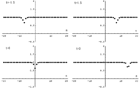
Figure 2: Plots of travelling 1-gray soliton. The vertical axis is $|\psi_{n}|$. ((a) $a=2,r=\exp(3{\rm i}\pi/4),\theta=5\pi/3$.)

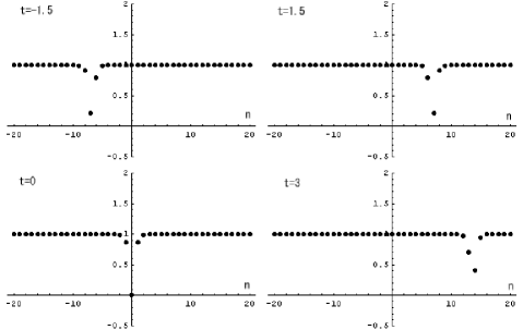
Figure 3: Plots of travelling 1-black soliton. The vertical axis is $|\psi_{n}|$. ($a=2,r=\exp(-5{\rm i}\pi/3),\theta=5\pi/3$.)

The 2-soliton solution is obtained by taking $N=2$ in eqs. (86) and (87). Similarly by rewriting as $p_{i}\to p_{i}\exp({\rm i}\theta)$ and $r_{i}\to r_{i}\exp({\rm i}\theta)$, we get an explicit expression of the 2-soliton solution for eq. (91),

$$\psi_{n}={G_{n}\over F_{n}}\exp({\rm i}(\theta n-2t\cos\theta))\,,$$

$$F_{n}=1+|p_{1}|^{2n}\exp(\xi_{1}+\xi_{1}^{*})+|p_{2}|^{2n}\exp(\xi_{2}+\xi_{2}^{*})$$

$$+\left|{p_{1}-p_{2}\over p_{1}p_{2}^{*}-1}\right|^{2}|p_{1}p_{2}|^{2n}\exp(\xi_{1}+\xi_{1}^{*}+\xi_{2}+\xi_{2}^{*})\,,$$

$$G_{n}=1-{p_{1}\over p_{1}^{*}r_{1}^{2}}|p_{1}|^{2n}\exp(\xi_{1}+\xi_{1}^{*})-{p_{2}\over p_{2}^{*}r_{2}^{2}}|p_{2}|^{2n}\exp({\xi_{2}+\xi_{2}^{*}})$$

$$\qquad+\left|{p_{1}-p_{2}\over p_{1}p_{2}^{*}-1}\right|^{2}{p_{1}\over p_{1}^{*}r_{1}^{2}}{p_{2}\over p_{2}^{*}r_{2}^{2}}|p_{1}p_{2}|^{2n}\exp(\xi_{1}+\xi_{1}^{*}+\xi_{2}+\xi_{2}^{*})\,,$$

where

$$\xi_{i}={\rm i}a\left(p_{i}+{1\over p_{i}}\right)t+\xi_{i0},\qquad p_{i}=a\exp(-{\rm i}\theta)+\sqrt{a^{2}-1}r_{i},\qquad|r_{i}|=1\,.$$

Here the carrier wave of the dark soliton solution is given by the exponential factor, $\exp({\rm i}(\theta n-2t\cos\theta))$. Figure 4 shows 2-dark soliton interaction.

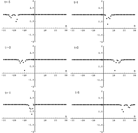
Figure 4: Plots of 2-dark soliton interaction. The vertical axis is $|\psi_{n}|$. ($a=2,r_{1}=\exp(3{\rm i}\pi/4),r_{2}=\exp({\rm i}\pi/4),\theta=5\pi/4$)

7 Concluding Remarks

We have shown that the $N$-dark soliton solutions of the IDNLS equation are given by the Casorati determinant. From the above derivation of the $N$-dark soliton solutions for the IDNLS equation, we notice that there is correspondence between the Casorati determinant solutions of the IDNLS equation and the RTL equation [18]. The RTL equation is decomposed into three bilinear equations, i.e. the Toda lattice (TL) equation, the Bäcklund transformation (BT) for TL and the DTL equation (See appendix A A). The IDNLS equation is also decomposed into three bilinear equations, i.e. two types of the BT for TL and the DTL equation.

This fact reminds us several works on the relationship between IDNLS and RTL [16, 17, 10]. Moreover, our result is an answer to an open problem of ref.Sadakane, i.e., the $N$-bright soliton solutions of IDNLS are written by the 2-component Casorati determinant in ref.Sadakane, and the $N$-dark soliton solution are written by the single-component Casorati determinant which is given in this paper and corresponds to the solution of RTL in ref.OKMS.

It is interesting to investigate $N$-dark soliton solutions of the discrete time IDNLS equation. It will be reported in the forthcoming paper.

Appendix A Relativistic Toda Lattice

In this appendix we briefly explain $\tau$-functions of the RTL equation. The RTL equation

$$\frac{d^{2}q_{n}}{dt^{2}} = (1+{1\over{\rm c}}\dot{q}_{n-1})(1+{1\over{\rm c}}\dot{q}_{n}){\exp(q_{n-1}-q_{n})\over 1+{1\over{\rm c}^{2}}\exp(q_{n-1}-q_{n})}$$ (93)

$$- (1+{1\over{\rm c}}\dot{q}_{n})(1+{1\over{\rm c}}\dot{q}_{n+1}){\exp(q_{n}-q_{n+1})\over 1+{1\over{\rm c}^{2}}\exp(q_{n}-q_{n+1})},$$

where $q_{n}$ is the coordinates of $n$-th lattice point and ${\rm c}$ is the light speed, was introduced and studied by Ruijsenaars [21]. The RTL equation (93) is transformed into the three bilinear equations,

$$D_{x}^{2}f_{n}\cdot f_{n}=2({\bar{g}}_{n}g_{n}-f_{n}^{2}),$$

$$(aD_{x}-1)f_{n}\cdot f_{n-1}+{\bar{g}}_{n-1}g_{n}=0,$$ (94)

$${\bar{g}}_{n-1}g_{n+1}-f_{n}^{2}=a^{2}(f_{n+1}f_{n-1}-f_{n}^{2}),$$

through the variable transformations,

$$q_{n}=\log{f_{n-1}\over f_{n}},$$ (95)

$$t={\sqrt{1+{\rm c}^{2}}\over{\rm c}}x,$$ (96)

$${\rm c}={\sqrt{1-a^{2}}\over a}.$$ (97)

In eqs. (94), $g$ and $\bar{g}$ are the auxiliary variables and $D$ is the bilinear differential operator defined by

$$D_{x}^{k}f\cdot g=(\partial_{x}-\partial_{y})^{k}f(x)g(y)|_{y=x}.$$

Letting

$$f_{n}=\tau_{n}(n),\quad g_{n}=\tau_{n-1}(n),\quad{\bar{g}}_{n}=\tau_{n+1}(n),$$ (98)

we have three bilinear equations, the TL equation, the Bäcklund transformation (BT) for TL and the DTL equation,

$$D_{x}^{2}\tau_{n}(k)\cdot\tau_{n}(k)=2(\tau_{n+1}(k)\tau_{n-1}(k)-\tau_{n}(k)\tau_{n}(k)),$$

$$(aD_{x}-1)\tau_{n}(k)\cdot\tau_{n-1}(k-1)+\tau_{n}(k-1)\tau_{n-1}(k)=0,$$ (99)

$$\tau_{n}(k+1)\tau_{n}(k-1)-\tau_{n}(k)\tau_{n}(k)$$

$$\quad\quad=a^{2}(\tau_{n+1}(k+1)\tau_{n-1}(k-1)-\tau_{n}(k)\tau_{n}(k)).$$

Appendix B Proof of Eqs. (86)-(88)

Let us first consider the Casorati determinant $\displaystyle D=\det_{1\leq i,j\leq N}(p_{i}^{j-1}A_{i}+q_{i}^{j-1}B_{i})$. Since each row is sum of two vectors, the determinant is given by the sum of $2^{N}$ terms,

$$D=\left|\begin{matrix}B_{1}&q_{1}B_{1}&\cdots&q_{1}^{N-1}B_{1}\cr B_{2}&q_{2}B_{2}&\cdots&q_{2}^{N-1}B_{2}\cr\vdots&\vdots&&\vdots\cr B_{N}&q_{N}B_{N}&\cdots&q_{N}^{N-1}B_{N}\cr\end{matrix}\right|+\sum_{i_{1}=1}^{N}\left|\begin{matrix}B_{1}&q_{1}B_{1}&\cdots&q_{1}^{N-1}B_{1}\cr\vdots&\vdots&&\vdots\cr A_{i_{1}}&p_{i_{1}}A_{i_{1}}&\cdots&p_{i_{1}}^{N-1}A_{i_{1}}\cr\vdots&\vdots&&\vdots\cr B_{N}&q_{N}B_{N}&\cdots&q_{N}^{N-1}B_{N}\cr\end{matrix}\right|$$

$$+\sum_{1\leq i_{1}<i_{2}\leq N}\left|\begin{matrix}B_{1}&q_{1}B_{1}&\cdots&q_{1}^{N-1}B_{1}\cr\vdots&\vdots&&\vdots\cr A_{i_{1}}&p_{i_{1}}A_{i_{1}}&\cdots&p_{i_{1}}^{N-1}A_{i_{1}}\cr\vdots&\vdots&&\vdots\cr A_{i_{2}}&p_{i_{2}}A_{i_{2}}&\cdots&p_{i_{2}}^{N-1}A_{i_{2}}\cr\vdots&\vdots&&\vdots\cr B_{N}&q_{N}B_{N}&\cdots&q_{N}^{N-1}B_{N}\cr\end{matrix}\right|+\cdots+\left|\begin{matrix}A_{1}&p_{1}A_{1}&\cdots&p_{1}^{N-1}A_{1}\cr A_{2}&p_{2}A_{2}&\cdots&p_{2}^{N-1}A_{2}\cr\vdots&\vdots&&\vdots\cr A_{N}&p_{N}A_{N}&\cdots&p_{N}^{N-1}A_{N}\cr\end{matrix}\right|$$

$$=\Delta(q_{1},q_{2},\cdots,q_{N})\prod_{i=1}^{N}B_{i}+\sum_{i_{1}=1}^{N}\Delta(q_{1},\cdots,p_{i_{1}},\cdots,q_{N})A_{i_{1}}\prod_{{i=1\atop i\neq i_{1}}}^{N}B_{i}$$

$$+\sum_{1\leq i_{1}<i_{2}\leq N}\Delta(q_{1},\cdots,p_{i_{1}},\cdots,p_{i_{2}},\cdots,q_{N})A_{i_{1}}A_{i_{2}}\prod_{{i=1\atop i\neq i_{1},i_{2}}}^{N}B_{i}+\cdots$$

$$+\sum_{1\leq i_{1}<i_{2}<\cdots<i_{M}\leq N}\Delta(q_{1},\cdots,p_{i_{1}},\cdots,p_{i_{2}},\cdots,p_{i_{M}},\cdots,q_{N})A_{i_{1}}A_{i_{2}}\cdots A_{i_{M}}\prod_{{i=1\atop i\neq i_{1},i_{2},\cdots,i_{M}}}^{N}B_{i}$$

$$+\cdots+\Delta(p_{1},p_{2},\cdots,p_{N})\prod_{i=1}^{N}A_{i}$$

$$=\Delta(q_{1},q_{2},\cdots,q_{N})\prod_{i=1}^{N}B_{i}\left(1+\sum_{i_{1}=1}^{N}\frac{\Delta(q_{1},\cdots,p_{i_{1}},\cdots,q_{N})}{\Delta(q_{1},\cdots,q_{N})}\frac{A_{i_{1}}}{B_{i_{1}}}\right.$$

$$+\sum_{1\leq i_{1}<i_{2}\leq N}\frac{\Delta(q_{1},\cdots,p_{i_{1}},\cdots,p_{i_{2}},\cdots,q_{N})}{\Delta(q_{1},\cdots,q_{N})}\frac{A_{i_{1}}A_{i_{2}}}{B_{i_{1}}B_{i_{2}}}+\cdots$$

$$+\sum_{1\leq i_{1}<i_{2}<\cdots<i_{M}\leq N}\frac{\Delta(q_{1},\cdots,p_{i_{1}},\cdots,p_{i_{2}},\cdots,p_{i_{M}},\cdots,q_{N})}{\Delta(q_{1},\cdots,q_{N})}\prod_{\nu=1}^{M}\frac{A_{i_{\nu}}}{B_{i_{\nu}}}$$

$$\left.+\cdots+\frac{\Delta(p_{1},\cdots,p_{N})}{\Delta(q_{1},\cdots,q_{N})}\prod_{i=1}^{N}\frac{A_{i}}{B_{i}}\right),$$

where $\Delta$ is the Vandermonde determinant defined by

$$\Delta(x_{1},x_{2},\cdots,x_{N})=\prod_{N\geq i>j\geq 1}(x_{i}-x_{j}).$$

By rewriting as

$$B_{i}=\left(\prod_{{k=1\atop k\neq i}}^{N}{p_{i}-q_{k}\over q_{i}-q_{k}}\right)B^{\prime}_{i},$$

each term of the summation is given by

$$\frac{\Delta(q_{1},\cdots,p_{i_{1}},\cdots,p_{i_{2}},\cdots,p_{i_{M}},\cdots,q_{N})}{\Delta(q_{1},\cdots,q_{N})}\prod_{\nu=1}^{M}\frac{A_{i_{\nu}}}{B_{i_{\nu}}}$$

$$=\frac{\Delta(p_{i_{1}},p_{i_{2}},\cdots,p_{i_{M}})}{\Delta(q_{i_{1}},q_{i_{2}},\cdots,q_{i_{M}})}\left(\prod_{\nu=1}^{M}\prod_{{j=1\atop j\neq i_{1},i_{2},\cdots,i_{M}}}^{N}{p_{i_{\nu}}-q_{j}\over q_{i_{\nu}}-q_{j}}\right)\prod_{\nu=1}^{M}\left(\prod_{{k=1\atop k\neq{i_{\nu}}}}^{N}{q_{i_{\nu}}-q_{k}\over p_{i_{\nu}}-q_{k}}\right)\frac{A_{i_{\nu}}}{B^{\prime}_{i_{\nu}}}$$

$$=\frac{\Delta(p_{i_{1}},p_{i_{2}},\cdots,p_{i_{M}})}{\Delta(q_{i_{1}},q_{i_{2}},\cdots,q_{i_{M}})}\left(\prod_{\nu=1}^{M}\prod_{{\mu=1\atop\mu\neq\nu}}^{M}{q_{i_{\nu}}-q_{i_{\mu}}\over p_{i_{\nu}}-q_{i_{\mu}}}\right)\prod_{\nu=1}^{M}\frac{A_{i_{\nu}}}{B^{\prime}_{i_{\nu}}}=\left(\prod_{1\leq\mu<\nu\leq M}{(p_{i_{\mu}}-p_{i_{\nu}})(q_{i_{\mu}}-q_{i_{\nu}})\over(p_{i_{\mu}}-q_{i_{\nu}})(q_{i_{\mu}}-p_{i_{\nu}})}\right)\prod_{\nu=1}^{M}\frac{A_{i_{\nu}}}{B^{\prime}_{i_{\nu}}},$$

thus we obtain

$$D=\left(\Delta(q_{1},q_{2},\cdots,q_{N})\prod_{i=1}^{N}B_{i}\right)\sum_{M=0}^{N}\ \sum_{1\leq i_{1}<i_{2}<\cdots<i_{M}\leq N}\left(\prod_{1\leq\mu<\nu\leq M}{(p_{i_{\mu}}-p_{i_{\nu}})(q_{i_{\mu}}-q_{i_{\nu}})\over(p_{i_{\mu}}-q_{i_{\nu}})(q_{i_{\mu}}-p_{i_{\nu}})}\right)\prod_{\nu=1}^{M}\frac{A_{i_{\nu}}}{B^{\prime}_{i_{\nu}}}.$$

The prefactor of above summation gives the gauge factor in eq. (85), and from the summation part, $F_{n}$, $G_{n}$ and $H_{n}$ in eqs. (86)-(88) are derived by taking

$$q_{i}={1\over p_{i}^{*}},\qquad p_{i}=a+\sqrt{a^{2}-1}r_{i},\qquad|r_{i}|=1,$$

and

$$\begin{array}[]{lll}A_{i}=p_{i}^{n}\exp(\xi_{i}),&\displaystyle B^{\prime}_{i}={1\over{p_{i}^{*}}^{n}}\exp(-\xi_{i}^{*}),&\hbox{for }F_{n},\\[10.0pt] \displaystyle A_{i}={p_{i}^{n+1}\over 1-ap_{i}}\exp(\xi_{i}),&\displaystyle B^{\prime}_{i}={1\over{p_{i}^{*}}^{n+1}(1-a/p_{i}^{*})}\exp(-\xi_{i}^{*}),&\hbox{for }G_{n},\\[10.0pt] A_{i}=p_{i}^{n-1}(1-ap_{i})\exp(\xi_{i}),&\displaystyle B^{\prime}_{i}={1-a/p_{i}^{*}\over{p_{i}^{*}}^{n-1}}\exp(-\xi_{i}^{*}),&\hbox{for }H_{n}.\end{array}$$

References

- [1] M. J. Ablowitz, B. Prinari and A. D. Trubatch: Discrete and Continuous Nonlinear Schrödinger Systems (Cambridge University Press, 2004).
- [2] P. G. Kevrekidis, K. O. Rasmussen and A. R. Bishop: Int. J. Mod. Phys. B, 15 (2001) 2833.
- [3] M. J. Ablowitz and J. F. Ladik: J. Math. Phys. 16 (1975) 598.
- [4] M. J. Ablowitz and J. F. Ladik: J. Math. Phys. 17 (1976) 1011.
- [5] R. Hirota: The Direct Method in Soliton Theory (Cambridge University Press, Cambridge, 2004).
- [6] R. Hirota: unpublished work.
- [7] S. Tsujimoto: Applied Integrable Systems, ed. Y. Nakamura (Shokabo, Tokyo, 2000) Chapter 1 [in Japanese].
- [8] K. Narita, J. Phys. Soc. Jpn. 59 (1990) 3528.
- [9] Y. Ohta: Chaos, Solitons & Fractals, 11 (2000) 91.
- [10] T. Sadakane: J. Phys. A: Math. Gen. 36 (2003) 87.
- [11] Y. Kivshar and W. Królikowski: Phys. Rev. E 50 (1994) 5020.
- [12] B. Sanchez-Rey and M. Johansson: Phys. Rev. E 71 (2005) 036627.
- [13] P. G. Kevrekidis, R. Carretero-González, G. Theocharis, D. J. Frantzeskakis and B. A. Malomed: Phys. Rev. E 68 (2003) 035602.
- [14] K. Narita: J. Phys. Soc. Jpn. 60 (1991) 1497.
- [15] V. E. Vekslerchik and V. V. Konotop: Inv. Prob. 8 (1992) 889.
- [16] V. E. Vekslerchik: Inv. Prob. 11 (1995) 463.
- [17] S. Kharchev, A. Mironov and A. Zhedanov: Int. J. Mod. Phys. A, 12 (1997) 2675.
- [18] Y. Ohta, K. Kajiwara, J. Matsukidaira and J. Satsuma: J. Math. Phys. 34 (1993) 5190.
- [19] N. C. Freeman and J. J. C. Nimmo: Phys. Lett. A 95 (1983) 1.
- [20] N. C. Freeman and J. J. C. Nimmo: Proc. Roy. Soc. London Ser. A 389 (1983) 319.
- [21] S. N. M. Ruijsenaars: Commun. Math. Phys. 133 (1990) 217.