Correlation functions of impedance and scattering matrix elements in chaotic absorbing cavities

Abstract

Wave scattering in chaotic systems with a uniform energy loss (absorption) is considered. Within the random matrix approach we calculate exactly the energy correlation functions of different matrix elements of impedance or scattering matrices for systems with preserved or broken time-reversal symmetry. The obtained results are valid at any number of arbitrary open scattering channels and arbitrary absorption. Elastic enhancement factors (defined through the ratio of the corresponding variance in reflection to that in transmission) are also discussed.

1 Introduction

Propagation of electromagnetic or ultrasonic waves in billiards [1], scattering of light in random media and transport of electrons through quantum dots [2, 3] share at least one feature in common: In all these situations one deals with an open wave-chaotic system studied by means of a scattering experiment, see Fig. 1 for an illustration. Here, we have a typical transport problem where the fundamental object of interest is the scattering matrix $S$, which relates linearly the amplitudes of incoming and outgoing fluxes. However, under real laboratory conditions there is a number of different sources which cause that a part of the flux gets irreversibly lost or dissolved in the environment. As a result, we encounter absorption and have to handle the $S$-matrix, which is no longer unitary. Statistics of different scattering observables in the presence of absorption are nowadays under intense experimental and theoretical studies. One should mention, in particular, experiments on energy correlations of the $S$-matrix [4, 5] and total cross-sections [6], distributions of reflection [4, 7] and transmission [8] as well as that of the complete $S$ matrix [9] in microwave cavities, properties of resonance widths [10] in such systems at room temperatures, dissipation of ultrasonic energy in elastodynamic billiards [11], fluctuations in microwave networks [12] (see also references in these papers). Theoretically, statistics of reflection, delay times and related quantities were considered first in the strong [13] or weak [14] absorption limits at perfect coupling, and very recently at arbitrary absorption and coupling [15, 16, 17, 18, 19].

Another insight to the same problem comes by considering it not from the “outside”, but rather from “inside”. Then the impedance relating linearly a voltage to a current turns out to be the prime object of interest [20, 21], see Fig. 1. It turns out that after proper taking into account of the wave nature of the current [22, 23], the cavity impedance becomes an electromagnetic analogue of Wigner’s reaction ($R$) matrix of the scattering theory. This can be understood qualitatively through the well-known equivalence of the two-dimensional Maxwell equations to the Schrödinger equation, the role of the wave function being played by the field (the voltage in our case). Then the definition of the impedance becomes formally similar to the definition of the $R$-matrix (which relates linearly the normal derivative of the wave function to the wave function itself on the boundary). The impedance is, therefore, related to the local Green function of the closed cavity and fluctuates strongly due to chaotic internal dynamics.

The imaginary part of the local Green function (which is proportional to the real part of the impedance) is known in the context of mesoscopics as the local density of states and has a long story of study, see [24] for a recent review. Actually, a closely related quantity in the context of spectra of complex atoms and molecules has the meaning of the total cross-section of indirect photoabsorption, see e.g. [25]. As to the real part, it seems to have no direct physical meaning in mesoscopics while it has the meaning of reactance in electromagnetics, where both real and imaginary parts are experimentally studied. Very recently an approach [26, 27] has been developed by us which allows one to study the (joint) distribution function of these real and imaginary parts at arbitrary absorption and to relate it to the reflection distribution, thus linking somewhat complementary experiments [9] and [20] together.

 

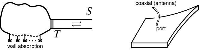
Figure 1: A sketch of a typical experimental setup with microwave billiards. A flat chaotic cavity is feeded with microwaves through an attached coaxial cable (i.e. a scattering channel). On average, $1-T$ part of the incoming flux, where $T\leq 1$ is the so-called transmission coefficient, is reflected back directly from the cable-cavity interface (port) without exciting long-lived resonances in the cavity. If the cavity is thin enough then only a transverse electric wave can propagate inside. The electric field has only a vertical component, which is uniform in vertical direction and distributed nontrivially in the plane. Therefore, there is a voltage between plates as well as a current due to the in-plane magnetic field. The impedance is a quantity which relates linearly the port voltage to the port current. Fluctuations of eigenmodes and eigenfrequencies result in fluctuations of the impedance or $S$-matrix, as the driving frequency or port position is changed.

Due to a strong resonance energy dependence the impedance and $S$-matrix as well as any scattering observable exhibit strong fluctuations over a smooth regular background as the scattering energy (or another external parameter) is varied. These two variations occurring on different energy scales are usually decomposed into a mean and a fluctuating part by means of the spectral or (assumed to be equivalent) ensemble average $\langle\cdots\rangle$. In this paper we consider statistics as determined by a two-point correlation function of the fluctuating parts (also called a “connected” correlator): $\left\langle AB\right\rangle_{\mathrm{conn}}=\left\langle AB\right\rangle-\left\langle A\right\rangle\left\langle B\right\rangle$. We restrict ourselves below to the cases of preserved and broken time-reversal symmetry (TRS).

2 Scattering, RMT and absorption

The resonance energy dependence of observables becomes explicit in the well-known Hamiltonian approach to quantum scattering, which was developed first in the context of nuclear physics [28, 29, 30] and adopted later for the needs of mesoscopic physics, see e.g. [3, 31, 32]. This framework is adequate to take finite absorption into account as well. We have the following relation between the resonance part of the scattering matrix and Wigner’s reaction matrix:

$$S(E)=\frac{1-\rmi K(E)}{1+\rmi K(E)}\,,\qquad K(E)={\textstyle\frac{1}{2}}V^{{\dagger}}(E-H)^{-1}V\,.$$ (1)

The Hamiltonian $H$ of the closed system gives rise to $N$ levels (eigenfrequencies) which are coupled to $M$ continuum channels via the $N{\times}M$ matrix $V$ of coupling amplitudes $V^{c}_{n}$ ($n=1\ldots N$, $c=1\ldots M$). Performing for $S$ a Taylor series expansion in $K$ and regrouping the terms, one comes to another well-known expression for the $S$ matrix

$$S(E)=1-\rmi V^{{\dagger}}\frac{1}{E-\mathcal{H}_{\mathrm{eff}}}V\,,\qquad\mathcal{H}_{\mathrm{eff}}=H-{\textstyle\frac{\rmi}{2}}VV^{{\dagger}}\,.$$ (2)

in terms of the effective Hamiltonian $\mathcal{H}_{\mathrm{eff}}$ of the open system, which is non-Hermitian contrary to the Hermitian $H$. The factorized structure of the anti-Hermitian part ensures the unitarity of $S(E)$ at real values of $E$. In a resonance approximation of the energy-independent amplitudes the complex eigenvalues $\mathcal{E}_{n}=E_{n}-{\textstyle\frac{\rmi}{2}}\Gamma_{n}$ of $\mathcal{H}_{\mathrm{eff}}$ are the only singularities of the $S$ matrix in the complex energy plane. As required by causality [33], they are located in the lower half plane and correspond to the long-lived resonance states, with energies $E_{n}$ and escape widths $\Gamma_{n}>0$, which are formed on the intermediate stage of a scattering process.

To mimic chaotic nature of the intrinsic motion we adopt, as usual, the random matrix theory (RMT) [2, 34, 35] and replace the actual Hamiltonian with a random Hermitian matrix $H$. It turns out that spectral fluctuations possess a large degree of universality in the limit $N{\to}\infty$: being expressed (“unfolding”) in units of the mean level spacing $\Delta$ they become independent of microscopic details (i.e. a particular form of the distribution of $H$) and get uniformly distributed throughout the whole spectrum [35]. That amounts usually to considering local fluctuations at the center of the spectrum ($E=0$) and to restricting ourselves to the simplest case of Gaussian ensembles. On has the Gaussian Orthogonal Ensemble (GOE, the Dyson’s symmetry index $\beta=1$ and $H$ symmetric) for chaotic systems with preserved time-reversal symmetry (TRS) and the Gaussian Unitary Ensemble (GUE, $\beta=2$ and $H$ Hermitian) for those with fully broken TRS. For similar reasons the approach is independent of particular statistical assumptions on coupling amplitudes $V^{a}_{n}$ (as long as $M\ll N$ [36, 37]), which may be chosen as fixed [29] or random [30] variables. They enter final expressions only by means of $M$ transmission coefficients (also so-called sticking probabilities)

$$T_{c}\equiv 1-|\overline{S^{cc}}|^{2}=\frac{4\kappa_{c}}{(1+\kappa_{c})^{2}}\,,\qquad\kappa_{c}=\frac{\pi\|V^{c}\|^{2}}{2N\Delta}\,.$$ (3)

where $\overline{S^{cc}}$ stands for the average (or “optical”) $S$ matrix. They are assumed to be input parameters of the theory. $T_{c}\ll 1$ or $T_{c}=1$ corresponds to an almost closed or perfectly open channel “c”, respectively.

Absorption is usually seen as a dissipation process, which evolves exponentially in time. Strictly speaking, different spectral components of the field have different dissipation rates. However, this rather weak energy dependence can easily be neglected as long as local fluctuations on much finer energy scale $\sim\Delta$ are considered. As a result, all the resonances acquire additionally to their escape widths one and the same absorption width $\Gamma>0$. The dimensionless parameter $\gamma\equiv 2\pi\Gamma/\Delta$ characterizes then the absorption strength, with $\gamma\ll 1$ or $\gamma\gg 1$ corresponding to the weak or strong absorption limit, respectively. (Microscopically, it can be modelled by means of a huge number of weakly open parasitic channels [5, 38] or by additional coupling to very complicated background with almost continuous spectrum [15], see also [39].)

Treating $\Gamma$ phenomenologically, one sees that such a uniform absorption can equivalently be taken into account by a purely imaginary shift of the scattering energy $E\to E+{\textstyle\frac{\rmi}{2}}\Gamma\equiv E_{\gamma}$, so that the $S$-matrix $S_{\gamma}(E)\equiv S(E_{\gamma})$ becomes subunitary. The reflection matrix $S_{\gamma}^{{\dagger}}S_{\gamma}<1$ provides then a natural measure of the mismatch between incoming and outgoing fluxes [14, 15]. At last but not least, the matrix $Z\equiv\rmi K(E_{\gamma})$ has the meaning of the normalized cavity impedance in such a setting, see [22, 23] for further details.

3 Correlation functions

3.1 Impedance

Let us consider first the simplest case of the impedance when the problem can be fully reduced to that of spectral correlations determined by the two-point cluster function $Y_{2,\beta}(\omega)=\delta(\omega)-\Delta^{2}\left\langle\rho(E_{1})\rho(E_{2})\right\rangle_{\mathrm{conn}}$, where $\omega=(E_{2}-E_{1})/\Delta$ and $\rho(E)$ being the spectral density. It is easy to find $\left\langle Z^{ab}\right\rangle=\kappa_{a}\delta^{ab}$ for the mean impedance at $E=0$. To calculate the energy correlation function

$$C^{abcd}_{Z}(\omega)\equiv\left\langle Z^{ab*}(E_{1})Z^{cd}(E_{2})\right\rangle_{\mathrm{conn}}$$ (4)

it is instructive to write $Z^{ab}(E)={\textstyle\frac{\rmi}{2}}\sum_{n}\frac{v^{a*}_{n}v^{b}_{n}}{E-E_{n}+\rmi\Gamma/2}$ in the eigenbasis of the closed system. The rotation that diagonalizes the random $H$ transforms the (fixed) coupling amplitudes $V^{a}_{n}$ to gaussian distributed random coupling amplitudes $v^{a}_{n}$ with the zero mean and the second moment $\left\langle v^{a*}_{n}v^{b}_{m}\right\rangle=(2\kappa_{a}\Delta/\pi)\delta^{ab}\delta_{nm}$. In such a representation (4) acquires the following form:

$$C^{abcd}_{Z}(\omega)=\sum_{n,m}\frac{1}{4}\left\langle v^{a}_{n}v^{b*}_{n}v^{c*}_{m}v^{d}_{m}\right\rangle\left\langle\frac{1}{E_{1}-E_{n}-{\textstyle\frac{\rmi}{2}}\Gamma}\frac{1}{E_{2}-E_{m}+{\textstyle\frac{\rmi}{2}}\Gamma}\right\rangle_{\mathrm{conn}}$$ (5)

so that averaging over coupling amplitudes (i.e. eigenfunctions) and that over the spectrum can be done independently. The gaussian statistics of $v$ results in

$${\textstyle\frac{1}{4}}({\textstyle\frac{\pi}{\Delta}})^{2}\left\langle v^{a}_{n}v^{b*}_{n}v^{c*}_{m}v^{d}_{m}\right\rangle=\kappa_{a}\kappa_{c}\delta^{ab}\delta^{cd}+\kappa_{a}\kappa_{b}(\delta^{ac}\delta^{bd}+\delta_{1\beta}\delta^{ad}\delta^{bc})\delta_{nm}$$ (6)

where $\delta_{1\beta}$ term accounts for the presence of TRS, when all $v^{a}_{n}$ are real and $Z$ is symmetric. It is useful then to represent the spectral correlator in the form of the Fourier integral $\int_{0}^{\infty}\rmd t_{1}\int_{0}^{\infty}\rmd t_{2}e^{-\Gamma(t_{1}+t_{2})/2}e^{\rmi E(t_{2}-t_{1})}e^{\rmi(E_{2}-E_{1})(t_{1}+t_{2})/2}\left\langle e^{\rmi(E_{n}t_{1}-E_{m}t_{2})}\right\rangle_{\mathrm{conn}}$. Due to the uniformity of local fluctuations in the bulk of the spectrum, one can integrate additionally over the position $E$ of the mean energy: $\int\!\frac{\rmd E}{N\Delta}e^{\rmi E(t_{2}-t_{1})}={\textstyle\frac{1}{N}}\delta(\frac{t_{2}-t_{1}}{t_{H}})$, where $t_{H}\equiv 2\pi/\Delta$ is the Heisenberg time. From the known RMT spectral fluctuations one also has $(1-N)\left\langle e^{\rmi(E_{n}-E_{m})t}\right\rangle_{\mathrm{conn}}=b_{2,\beta}(t/t_{H})$ for $n{\neq}m$, where $b_{2,\beta}(\tau)$ is the spectral form factor defined through the Fourier transform of $Y_{2,\beta}(\omega)$ [34, 35]:

$$b_{2,\beta=1}(\tau)=[1-2\tau+\tau\log(1+2\tau)]\Theta(1-\tau)+[\tau\log({\textstyle\frac{2\tau+1}{2\tau-1}})-1]\Theta(\tau-1)$$ (7a)

$$b_{2,\beta=2}(\tau)=(1-\tau)\Theta(1-\tau)$$ (7b)

at $\tau>0$ and $b_{2,\beta}(-\tau)=b_{2,\beta}(\tau)$, so that $Y_{2,\beta}(\omega)=\int_{-\infty}^{\infty}\!\rmd\tau e^{2\pi\rmi\omega\tau}b_{2,\beta}(\tau)$. Combining all these results together and measuring the time in units of the Heisenberg time ($\tau=t/t_{H}$), we arrive finally at

$$C^{abcd}_{Z}(\omega)=\int_{0}^{\infty}\!\!\!\rmd\tau e^{2\pi\rmi\omega\tau}C^{abcd}_{Z}(\tau)$$ (7ha)

$$C^{abcd}_{Z}(\tau)=4\,e^{-\gamma\tau}\,[\kappa_{a}\kappa_{c}(1-b_{2,\beta}(\tau))\delta^{ab}\delta^{cd}+\kappa_{a}\kappa_{b}(\delta^{ac}\delta^{bd}+\delta_{1\beta}\delta^{ad}\delta^{bc})]\,.$$ (7hb)

Similar in spirit calculations were done earlier a context of reverberation in complex structures in [40, 41] and in a context of chaotic photodissociation in [42, 43].

The form factor (7hb) is simply related to that of $K$ matrix elements at zero absorption as $C^{abcd}_{Z}(\tau)=e^{-\gamma\tau}C^{abcd}_{K}(\tau)$. Such a relationship between the corresponding form factors with and without absorption is generally valid for any correlation function which may be reduced to the two-point correlator of resolvents (see [6] and below, e.g., for the case of the $S$ matrix). This can be easily understood as the result of the analytic continuation $2\pi\omega\to 2\pi\omega+i\gamma$ of the energy difference $\omega$ when absorption is switched on (see the previous section).

 

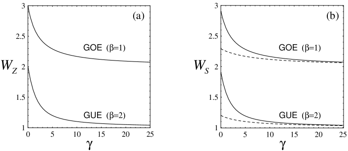
Figure 2: The impedance (a) and $S$-matrix (b) enhancement factors for chaotic systems with preserved ($\beta=1$) or broken ($\beta=2$) time-reversal symmetry as functions of the absorption strength $\gamma$. The case (b) corresponds to the many-channel limit with isolated ($\sum_{c}T_{c}=0.2$, solid lines) or overlapping resonances ($\sum_{c}T_{c}=5$, dashed lines).

The obtained expressions describe a decorrelation process of the $Z$ matrix elements as the energy difference grows, generally, $C_{Z}(\omega{\to}\infty)\to 0$. At $\omega=0$, (7ha) provides us with impedance variances $C_{Z}^{abab}(0)=\mathrm{var}(Z^{ab})\equiv\langle|Z^{ab}|^{2}\rangle-|\langle{Z^{ab}}\rangle|^{2}$, which were recently studied in [44] (see also [45]). In analogy with the so-called elastic enhancement factor considered frequently in nuclear physics [46], one can define the following ratio of variances in reflection ($a{=}b$) to that in transmission ($a{\neq}b$):

$$W_{Z,\beta}\equiv\frac{\sqrt{\mathrm{var}(Z^{aa})\mathrm{var}(Z^{bb})}}{\mathrm{var}(Z^{ab})}=2+\delta_{1\beta}-\int_{0}^{\infty}\!\!\rmd s\,e^{-s}b_{2,\beta}({\textstyle\frac{s}{\gamma}})$$ (7hi)

where the second equality follows easily from (7hb) (note that the coupling constants $\kappa_{a,b}$ are mutually cancelled here). Making use of $b_{2,\beta}(\infty){=}0$ and $b_{2,\beta}(0){=}1$, one can readily find $W_{Z,\beta}$ in the limiting cases of weak or strong absorption as:

$$W_{Z,\beta}=\cases{2+\delta_{1\beta}&at $\gamma\ll 1$\\ 1+\delta_{1\beta}&at $\gamma\gg 1$\\ }\,.$$ (7hj)

$W_{Z,\beta}$ decays monotonically as absorption grows, see Fig. 1a. In the case of unitary symmetry, (7b) and (7hi) yield explicitly $W_{Z,2}=1+{\textstyle\frac{1}{\gamma}}(1-e^{-\gamma})$ in agreement with [44]. It is hardly possible to get a simple explicit expression at finite $\gamma$ in the case of orthogonal symmetry. However, a reasonable approximation can be found if one notices that the integration in (7hi) is determined mainly by the region $s\leq 1$, so that one can approximate $b_{2,1}(s)\approx(1-2s+2s^{2})\Theta(1-s)$ through its Taylor expansion. Performing the integration, one arrives at $W_{Z,1}\approx 3-\gamma^{-2}[(4+\gamma^{2})(1-e^{-\gamma})-2\gamma(1+e^{-\gamma})]$, which turns out to be a good approximation to the exact answer at moderate absorption (deviations are seen numerically only at $\gamma\sim 1$).

3.2 $S$-matrix elements

The energy correlation function of the scattering matrix elements

$$C^{abcd}_{S}(\omega)\equiv\left\langle S_{\gamma}^{ab*}(E_{1})S_{\gamma}^{cd}(E_{2})\right\rangle_{\mathrm{conn}}=\int_{0}^{\infty}\!\!\rmd\tau e^{2\pi\rmi\omega\tau}C^{abcd}_{S}(\tau)$$ (7hk)

is a much more complicated object for an analytical treatment as (4). The reason becomes clearer if one considers again the pole representation of the $S$ matrix which follows from (2): $S^{ab}(E)=\delta^{ab}-\rmi\sum{w^{a}_{n}\tilde{w}^{b}_{n}}/(E-\mathcal{E}_{n})$. Due to a unitarity constraint imposed on $S$ (at real $E$), the residues and complex energies get mutually correlated [30] with a generally unknown joint distribution. The separation like (5) into a “coupling” and “spectral” average in no longer possible and can be done only by involving some approximations [47]. The powerful supersymmetry method [29, 48] turns out to be an appropriate technique to perform the statistical average in this case. In their seminal paper [29], Verbaarschot, Weidenmüller and Zirnbauer performed the exact calculation of (7hk) at arbitrary transmission coefficients (and zero absorption) in the case of orthogonal symmetry. This finding was later adopted [6] to include absorption. The corresponding exact result for unitary symmetry is still lacking in the literature (see, however, [49] concerning the $S$-matrix variance in the GOE-GUE crossover at perfect coupling) and will be presented below.

The calculation proceeds alone the same line as in [29], we indicate only essential differences. As usual, the representation of resolvents and thus (7hk) in the form of gaussian integrals over auxiliary “supervectors” consisting of both commuting and anticommuting (Grassmann) variables allows one to perform statistical averaging exactly. In the limit $N\to\infty$, the rest integration over the auxiliary field can be done in the saddle-point approximation. The final expression for both the correlator and its form factor (7hk) can be equally represented as follows:

$$C^{abcd}_{S}=\delta^{ab}\delta^{cd}T_{a}T_{c}\sqrt{(1-T_{a})(1-T_{c})}J_{ac}+(\delta^{ac}\delta^{bd}+\delta_{1\beta}\delta^{ad}\delta^{bc})T_{a}T_{b}P_{ab}\,.$$ (7hl)

Here, the $\delta_{1\beta}$ term accounts trivially for the symmetry property $S^{ab}=S^{ba}$ in the presence of TRS. $J_{ac}$ and $P_{ab}$ defined below are some functions (of the energy difference $\omega$ or the time $\tau$), which depend also on TRS, coupling and absorption but already in a nontrivial way. As a result, the elastic enhancement factor $W_{S,\beta}\equiv\sqrt{\mathrm{var}(S^{aa})\mathrm{var}(S^{bb})}/\mathrm{var}(S^{ab})$ is generally a complicated function of all these parameters, in contrast to (7hi). In the particular case of perfect coupling, all $T_{c}=1$, one has obviously from (7hl) that $W_{S,\beta}=1+\delta_{1\beta}$ at any absorption strength.

The saddle-point integration turns out to have a nontrivial saddle-point manifold [48] over which one needs to integrate exactly. This task can be accomplished by making use of the “angular” parametrization [29] of the manifold in terms of the $\frac{4}{\beta}{\times}\frac{4}{\beta}$ supermatrices $t_{12}$ and $t_{21}$. We consider first real $\omega$ (no absorption). Then the functions $J_{ac}$ and $P_{ab}$ have in the energy domain the following representation:

$$J_{ac}(\omega)=\frac{\beta^{2}}{16}\left\langle\mathrm{str\,}\Bigl{[}\frac{t_{12}t_{21}}{1+T_{a}t_{12}t_{21}}k\Bigr{]}\,\mathrm{str\,}\Bigl{[}\frac{t_{21}t_{12}}{1+T_{c}t_{21}t_{12}}k\Bigr{]}\mathcal{F}^{(\beta)}_{M}\right\rangle_{\mu}$$ (7hma)

$$P_{ab}(\omega)=\frac{\beta}{16}\left\langle\mathrm{str\,}\Bigl{[}t_{21}\frac{(1+t_{12}t_{21})^{1/2}}{1+T_{a}t_{12}t_{21}}kt_{12}\frac{(1+t_{21}t_{12})^{1/2}}{1+T_{b}t_{21}t_{12}}k\Bigr{]}\mathcal{F}^{(\beta)}_{M}\right\rangle_{\mu}$$ (7hmb)

that is completely in a parallel with [29] (the diagonal matrix $k=1$ ($-1$) in the subspace of commuting (anticommuting) variables). This result has the form of an expectation value $\langle(\cdots)\rangle_{\mu}\equiv\int\!\rmd\mu_{(\beta)}(\cdots)e^{\rmi\mathcal{L_{\beta}}(\omega)}$ in the field theory (nonlinear “zero-dimensional” supersymmetric $\sigma$-model) characterized by the Lagrangian $\mathcal{L}_{\beta}(\omega)=\beta\pi\omega\,\mathrm{str\,}(t_{12}t_{21})$. The so-called channel factor $\mathcal{F}^{(\beta)}_{M}=\prod_{c=1}^{M}\mathrm{sdet\,}(1+T_{c}t_{12}t_{21})^{-\beta/2}$ accounts for system openness. We refer the reader to [29, 50] for a definition of the supertrace and superdeterminant as well as for a general discussion of the superalgebra. An explicit parametrization of matrices $t_{12},t_{21}$ and the integration measure $\rmd\mu_{(\beta)}$ over them depend on the symmetry case considered; it can be found in [29] for $\beta=1$ and in [51, 52] for $\beta=2$. Essential is that the final expressions are determined only by real “eigenvalues” $\mu_{0}$ and $\mu_{1,2}$ of the angular matrices. Finally, one can cast resulting expressions as follows

$$J_{ac}(\omega)=\textstyle\left\langle\bigl{(}\frac{\mu_{1}}{1+T_{a}\mu_{1}}+\frac{\mu_{2}}{1+T_{a}\mu_{2}}+\frac{\mu_{0}}{1-T_{a}\mu_{0}}\bigr{)}\bigl{(}\frac{\mu_{1}}{1+T_{c}\mu_{1}}+\frac{\mu_{2}}{1+T_{c}\mu_{2}}+\frac{\mu_{0}}{1-T_{c}\mu_{0}}\bigr{)}\mathcal{F}_{M}\right\rangle_{\mu}$$ (7hmna)

$$\textstyle P_{ab}(\omega)=\textstyle\left\langle\bigl{(}\frac{\mu_{1}(1+\mu_{1})}{(1+T_{a}\mu_{1})(1+T_{b}\mu_{1})}+\frac{\mu_{2}(1+\mu_{2})}{(1+T_{a}\mu_{2})(1+T_{b}\mu_{2})}+\frac{\mu_{0}(1-\mu_{0})}{(1-T_{a}\mu_{0})(1-T_{b}\mu_{0})}\bigr{)}\mathcal{F}_{M}\right\rangle_{\mu}$$ (7hmnb)

with $\mathcal{F}_{M}=\prod_{c}[\frac{(1-T_{c}\mu_{0})^{2}}{(1+T_{c}\mu_{1})(1+T_{c}\mu_{2})}]^{1/2}$ in the $\beta=1$ case of orthogonal symmetry [29], and

$$J_{ac}(\omega)=\textstyle\left\langle\bigl{(}\frac{\mu_{1}}{1+T_{a}\mu_{1}}+\frac{\mu_{0}}{1-T_{a}\mu_{0}}\bigr{)}\bigl{(}\frac{\mu_{1}}{1+T_{c}\mu_{1}}+\frac{\mu_{0}}{1-T_{c}\mu_{0}}\bigr{)}\mathcal{F}_{M}\right\rangle_{\mu}$$ (7hmnoa)

$$\textstyle P_{ab}(\omega)=\textstyle\left\langle\bigl{(}\frac{\mu_{1}(1+\mu_{1})}{(1+T_{a}\mu_{1})(1+T_{b}\mu_{1})}+\frac{\mu_{0}(1-\mu_{0})}{(1-T_{a}\mu_{0})(1-T_{b}\mu_{0})}\bigr{)}\mathcal{F}_{M}\right\rangle_{\mu}$$ (7hmnob)

with $\mathcal{F}_{M}=\prod_{c}\frac{1-T_{c}\mu_{0}}{1+T_{c}\mu_{1}}$ in the $\beta=2$ case of unitary symmetry. Here, the corresponding integration $\langle(\cdots)\rangle_{\mu}$ is to be understood explicitly for these two respective cases as

$$\frac{1}{8}\int_{0}^{\infty}\!\rmd\mu_{1}\!\int_{0}^{\infty}\!\rmd\mu_{2}\!\int_{0}^{1}\!\rmd\mu_{0}\frac{(1-\mu_{0})\mu_{0}|\mu_{1}-\mu_{2}|\,e^{\rmi\pi\omega(\mu_{1}+\mu_{2}+2\mu_{0})}}{[(1+\mu_{1})\mu_{1}(1+\mu_{2})\mu_{2}]^{1/2}(\mu_{0}+\mu_{1})^{2}(\mu_{0}+\mu_{2})^{2}}\left(\ldots\right)$$ (7hmnop)

and

$$\int_{0}^{\infty}\!\rmd\mu_{1}\int_{0}^{1}\!\rmd\mu_{0}(\mu_{1}+\mu_{0})^{-2}\,e^{\rmi 2\pi\omega(\mu_{1}+\mu_{0})}\left(\ldots\right)\,.$$ (7hmnoq)

In the important particular case of the single open channel (elastic scattering), the general expression for the $\beta=2$ case simplifies further to

$$\left\langle S^{*}(E_{1})S(E_{2})\right\rangle_{\mathrm{conn}}=T^{2}\int_{0}^{\infty}\!\rmd\mu_{1}\int_{0}^{1}\!\frac{\rmd\mu_{0}}{\mu_{1}+\mu_{0}}\frac{1+(2-T)\mu_{1}}{(1+T\mu_{1})^{3}}\,e^{\rmi 2\pi\omega(\mu_{1}+\mu_{0})}\,.$$ (7hmnor)

Finally, putting above $\omega\to\omega+\rmi\gamma/2\pi$ accounts for the finite absorption strength $\gamma$.

To consider (7hl) in the time domain, i.e. the form factor $C^{abcd}_{S}(\tau)$, we notice that the variable $\tau={\textstyle\frac{1}{2}}(\mu_{1}+\mu_{2}+2\mu_{0})$ for $\beta=1$ or $\tau=\mu_{1}+\mu_{0}$ for $\beta=2$ plays the role of the dimensionless time. The corresponding expressions for $P_{ab}(\tau)$ and $J_{ac}(\tau)$ can be investigated using the methods developed in [46, 47, 53]. For orthogonal symmetry it was done in [6], where the overall decaying factor $e^{-\gamma\tau}$ due to absorption was also confirmed by comparison to the experimental result for the form factor measured in microwave cavities. It is useful for the qualitative description to note that $P_{ab}(\tau)$ and $2J_{ac}(\tau)$ are quite similar to the “norm leakage” decay function [54] and the form factor of the Wigner’s time delays [37], respectively (they would coincide exactly at $\gamma=0$, if we put $T_{a,b,c}=0$ appearing explicitly in denominators of (7hma) and thereafter). Then one can follow analysis performed in these papers, see also [53], to find qualitatively $P_{ab}(\tau)\sim e^{-\gamma\tau}(1+{\textstyle\frac{2}{\beta}}T_{a}\tau)^{-1}(1+{\textstyle\frac{2}{\beta}}T_{b}\tau)^{-1}\prod_{c}(1+{\textstyle\frac{2}{\beta}}T_{c}\tau)^{-\beta/2}$ and $J_{ab}(\tau)\sim[1-b_{2,\beta}(\tau)]P_{ab}(\tau)$. One has $P_{ab}(\tau)\approx e^{-\gamma\tau}$ and $J_{ab}(\tau)\approx(2\tau/\beta)e^{-\gamma\tau}$ as exact asymptotic at small times [47], they both being $\sim e^{-\gamma\tau}\tau^{-M\beta/2-2}$ at large times.

Such a power law is characteristic for open systems [31, 53, 54]. Physically, it results from width fluctuations, which diminish as the number $M$ of open channels grows [32, 54]. In the limiting case $M\to\infty$ and $T_{c}\to 0$, all the resonances acquire just the same escape width (in units of $t_{H}^{-1}$) $\sum_{c}T_{c}$ , which is often called the Weisskopf’s width [55], so that the total width is $\gamma_{T}=\sum_{c}T_{c}+\gamma$. Then further simplifications occur: $P_{ab}(\tau)=e^{-\gamma_{T}\tau}$ and $J_{ab}(\tau)=[1-b_{2,\beta}(\tau)]e^{-\gamma_{T}\tau}$, that results finally in

$$C^{abcd}_{S}(\omega)=\frac{(\delta^{ac}\delta^{bd}+\delta_{1\beta}\delta^{ad}\delta^{bc})T_{a}T_{b}}{\gamma_{T}-2\pi\rmi\omega}+\delta^{ab}\delta^{cd}T_{a}T_{c}\int_{0}^{\infty}\!\rmd\tau[1-b_{2,\beta}(\tau)]e^{-(\gamma_{T}-2\pi\rmi\omega)\tau}.$$ (7hmnos)

For the case of $\beta=1$ this result (at zero absorption) was obtained earlier by Verbaarschot [46]. In the limit considered, expression (7hmnos) is very similar to (7ha), (7hb), so that the enhancement factor $W_{S,\beta}$ is given by the same (7hi) where $\gamma$ is to be substituted with $\gamma_{T}$, see Fig. 1(b) for an illustration. At $\gamma_{T}\gg 1$ (large resonance overlapping or strong absorption, or both) the dominating term in (7hmnos) is the first one, which is known as the Hauser-Feshbash relation [56], see [57, 58, 59] for discussion. Then $W_{S,\beta}=2/\beta=W_{Z,\beta}$ that can be also understood as the consequence of the gaussian statistics of $S$ (as well as of $Z$) in the limit of strong absorption [59].

4 Conclusions

For open wave chaotic systems with preserved or broken TRS we have calculated exactly the energy correlation function of impedance matrix elements at arbitrary absorption and coupling. This function is found to be related to the two-level cluster function, or to its form factor in the time domain. The overall exponential decay due to uniform absorption is shown to be the generic feature of any correlation function reduced to a two-point spectral (resolvent) correlator, that follows simply from analytic properties of the latter in the complex energy plane. The elastic enhancement factor defined though the ratio of variances in reflection to that in transmission diminishes gradually from the value $1+2/\beta$ at weak absorption to $2/\beta$ at strong absorption.

The similar exact calculation for $S$-matrix elements has been performed in the case of broken TRS, thus completing the well-known result [29] of preserved TRS. The corresponding enhancement factor never reaches the maximum value $1+2/\beta$ at any finite resonance overlapping. It attains the value $2/\beta$ in the limit of strong absorption (independent of coupling) or at perfect coupling (independent of absorption).

We thank S. Anlage, U. Kuhl and H.-J. Stöckmann for useful discussions. The financial support by the SFB/TR 12 der DFG (D.V.S. and H.-J.S.) and EPSRC grant EP/C515056/1 (Y.V.F.) is acknowledged.

References

- [1] Stöckmann H J 1999 Quantum Chaos: An Introduction (Cambridge, UK: Cambridge University Press).
- [2] Beenakker C W J 1997 Rev. Mod. Phys. 69 731.
- [3] Alhassid Y 2000 Rev. Mod. Phys. 72 895.
- [4] Doron E, Smilansky U and Frenkel A 1990 Phys. Rev. Lett. 65 3072.
- [5] Lewenkopf C H, Müller A and Doron E 1992 Phys. Rev. A 45 2635.
- [6] Schäfer R, Gorin T, Seligman T H and Stöckmann H J 2003 J. Phys. A: Math. Gen. 36 3289.
- [7] Méndez-Sánchez R A, Kuhl U, Barth M, Lewenkopf C H and Stöckmann H J 2003 Phys. Rev. Lett. 91 174102.
- [8] Schanze H, Stöckmann H J, Martínez-Mares M and Lewenkopf C H 2005 Phys. Rev. E 71 016223.
- [9] Kuhl U, Martínez-Mares M, Méndez-Sánchez R A and Stöckmann H J 2005 Phys. Rev. Lett. 94 144101.
- [10] Barthélemy J, Legrand O and Mortessagne F 2005 Phys. Rev. E 71 016205.
- [11] Lobkis O I, Rozhkov I S and Weaver R L 2003 Phys. Rev. Lett. 91 194101.
- [12] Hul O, Bauch S, Pakonski P, Savytskyy N, Zyczkowski K and Sirko L 2004 Phys. Rev. E 69 056205.
- [13] Kogan E, Mello P A and Liqun H 2000 Phys. Rev. E 61 R17.
- [14] Beenakker C W J and Brouwer P W 2001 Physica E 9 463.
- [15] Savin D V and Sommers H J 2003 Phys. Rev. E 68 036211.
- [16] Fyodorov Y V 2003 JETP Lett. 78 250.
- [17] Savin D V and Sommers H J 2004 Phys. Rev. E 69 035201(R).
- [18] Rozhkov I, Fyodorov Y V and Weaver R L 2003 Phys. Rev. E 68 016204.
- [19] Rozhkov I, Fyodorov Y V and Weaver R L 2004 Phys. Rev. E 69 036206.
- [20] Hemmady S, Zheng X, Ott E, Antonsen T M and Anlage S M 2005 Phys. Rev. Lett. 94 014102.
- [21] Hemmady S, Zheng X, Antonsen T M, Ott E and Anlage S M 2005 Phys. Rev. E 71 056215.
- [22] Zheng X, Antonsen T M and Ott E 2004 e-print cond–mat/0408327.
- [23] Zheng X, Antonsen T M and Ott E 2004 e-print cond–mat/0408317.
- [24] Mirlin A D 2000 Phys. Rep. 326 259.
- [25] Fyodorov Y V and Alhassid Y 1998 Phys. Rev. A 58 R3375.
- [26] Fyodorov Y V and Savin D V 2004 JETP Lett. 80 725. [Pis’ma v ZhETP 80, 855 (2004)].
- [27] Savin D V, Sommers H J and Fyodorov Y V 2005 e-print cond–mat/0502359.
- [28] Mahaux C and Weidenmüller H A 1969 Shell-model Approach to Nuclear Reactions (Amsterdam: North-Holland).
- [29] Verbaarschot J J M, Weidenmüller H A and Zirnbauer M R 1985 Phys. Rep. 129 367.
- [30] Sokolov V V and Zelevinsky V G 1989 Nucl. Phys. A 504 562.
- [31] Lewenkopf C H and Weidenmüller H A 1991 Ann. Phys. (N.Y.) 212 53.
- [32] Fyodorov Y V and Sommers H J 1997 J. Math. Phys. 38 1918.
- [33] Nussenzveig H M 1972 Causality and Dispersion Relations (New York: Academic Press).
- [34] Mehta M L 1991 Random Matrices. 2nd edn. (New York: Academic Press).
- [35] Guhr T, Müller-Groeling A and Weidenmüller H A 1998 Phys. Rep. 299 189.
- [36] Lehmann N, Saher D, Sokolov V V and Sommers H J 1995 Nucl. Phys. A 582 223.
- [37] Lehmann N, Savin D V, Sokolov V V and Sommers H J 1995 Physica D 86 572.
- [38] Brouwer P W and Beenakker C W J 1997 Phys. Rev. B 55 4695.
- [39] Sokolov V V 2004 e-print cond–mat/0409690.
- [40] Davy J L 1987 J. Sound Vib. 115 145.
- [41] Lobkis O I, Weaver R L and Rozhkov I S 2000 J. Sound Vib. 237 281.
- [42] Alhassid Y and Levine R D 1992 Phys. Rev. A 46 4650.
- [43] Alhassid Y and Fyodorov Y V 1998 J. Phys. Chem. A 102 9577.
- [44] Zheng X, Hemmady S, Antonsen T M, Anlage S M and Ott E 2005 e-print cond–mat/0504196.
- [45] Hemmady S, Zheng X, Antonsen T M, Ott E and Anlage S M 2005 e-print nlin.CD/0506025; to be published in Acta Phys. Pol. A (Proceedings of the 2nd Workshop on Quantum Chaos and Localization Phenomena, May 19–22, 2005, Warsaw).
- [46] Verbaarschot J J M 1986 Ann. Phys. (N.Y.) 168 368.
- [47] Gorin T and Seligman T H 2002 Phys. Rev. E 65 026214.
- [48] Efetov K B 1983 Adv. Phys. 32 53.
- [49] Pluhař Z, Weidenmüller H A, Zuk J A, Lewenkopf C H and Wegner F J 1995 Ann. Phys. (N.Y.) 243 1.
- [50] Efetov K B 1996 Supersymmetry in Disorder and Chaos (Cambridge, UK: Cambridge University Press).
- [51] Zuk J A 1994 e-print cond–mat/0412060.
- [52] Fyodorov Y V 1995 In E Akkermans, G Montambaux, J L Pichard and J Zinn-Justin, eds., Mesoscopic Quantum Physics, Proceedings of the Les-Houches Summer School, Session LXI, p. 493 (Elsevier).
- [53] Dittes F M 2000 Phys. Rep. 339 215.
- [54] Savin D V and Sokolov V V 1997 Phys. Rev. E 56 R4911.
- [55] Blatt J M and Weisskopf V F 1979 Theoretical Nuclear Physics (Berlin: Springer-Verlag).
- [56] Hauser W and Feshbach H 1952 Phys. Rev. 87 366.
- [57] Moldauer P A 1975 Phys. Rev. C 11 426.
- [58] Agassi D, Weidenmüller H A and Mantzouranis G 1975 Phys. Rep. 22 146.
- [59] Friedman W A and Mello P A 1985 Ann. Phys. (N.Y.) 161 276.