Chaos in computer performance

Abstract

Modern computer microprocessors are composed of hundreds of millions of transistors that interact through intricate protocols. Their performance during program execution may be highly variable and present aperiodic oscillations. In this paper, we apply current nonlinear time series analysis techniques to the performances of modern microprocessors during the execution of prototypical programs. Our results present pieces of evidence strongly supporting that the high variability of the performance dynamics during the execution of several programs display low-dimensional deterministic chaos, with sensitivity to initial conditions comparable to textbook models. Taken together, these results show that the instantaneous performances of modern microprocessors constitute a complex (or at least complicated) system and would benefit from analysis with modern tools of nonlinear and complexity science.

Modern microprocessor architectures rely on impressive numbers of transistors (up to a billion) that interact through intricate rules. As a consequence, the performance of these microprocessors during the execution of certain programs displays complex non-repetitive variations that challenge traditional analysis. Yet, comparable complex behaviors are observed in many other systems ranging from physics to biology and social sciences and have been successfully described using nonlinear and chaotic data analysis. In this paper, we apply these methods to analyze modern microprocessor performances. We collect several measures characterizing the architectural state and performance during the execution of several prototypical programs and apply current techniques of nonlinear analysis to the resulting time-varying signals. Our results show that for several programs, the complex and highly variable dynamics observed result from deterministic chaos. This suggests that detailed predictions of microprocessor performance is unlikely with these programs. Taken together, these results show that the instantaneous performances during program executions on modern microprocessor architectures form a byzantine system that should benefit from analysis with modern tools of nonlinear and complexity science.

I Introduction

Modern computer architectures result from a rapidly growing evolution that can be traced back to the 1960’s, when Moore observed that the number of transistors per integrated circuit displayed an exponential growth and predicted that this trend would continue Moore (1965). The so-called Moore’s Law has indeed been maintained during the last 40 years, as transistor density doubled approximately every 18 months. Consequently, today computer processors rely on amazingly high numbers of transistors: the widespread Intel®  Pentium®  4 contains 42 million transistors but the more recent Itanium®  2 possesses 410 million of them. Furthermore, a constant of this evolution is that processor speed (especially, its clock rate) by far outperforms memory operations. Hence, most recent advances in the field have mainly aimed at hiding memory latencies using engineering solutions (parallel executions, pipelining, cache memory systems). But this necessarily came with further increases of the processor complexity.
As a consequence, predicting the precise performance of microprocessors (the number of instructions executed each second) during execution of programs running on modern computer architectures has become increasingly difficult. For instance, one efficient way to optimize computer performance for a given program consists in fine-tuning the compiler options to adapt the compiler work to the considered architecture. Yet the complexity of modern architectures is such that rational optimizations, guided by a thorough knowledge of the architecture, are now less efficient, up to the point that more systematic automated search methods based on machine-learning Stephenson and Amarasinghe (2005), genetic algorithms Kulkarni et al. (2004) or iterative trial-and-error techniques Fursin et al. (2002) are being investigated as possible replacements.
Hence, on the basis of the high number of their components dedicated to performance improvement and the intricacy of their interactions, the instantaneous performance of modern microprocessors may be viewed as a complex system. As a consequence, performance recordings during the execution of certain programs can be highly variable Duesterwald et al. (2003) and difficult to predict Annavaram et al. (2004). Analyzing and predicting performance (i.e. the rate at which the microprocessor will execute a given program) has proven increasingly difficult.
Early on, computer architects dismissed modeling as inappropriate because it was too inaccurate to capture the slight performance differences between two architecture mechanisms. For instance, even modeling of a single non-trivial architecture component such as a cache memory spawned decades of research Slingerland and Smith (2001); Lam et al. (1991); Coleman and McKinley (1995); Gluhovsky and O’Krafka (2005), and proved only partially successful a few years ago for a range of programs with fairly regular behavior and simplistic architectures Abella et al. (2001). Instead, computer architects have always relied upon detailed simulators which describe the architecture behavior on every cycle Burger et al. (1996). As a consequence, simulators execute a program about 10000 times slower than on a real architecture, and this technique is now becoming overly time-consuming and inappropriate for complex processors and future processors with a large number of cores. Consequently, novel approaches to understanding and anticipating system behavior are currently sought in the computer architecture community Karkhanis and Smith (2004).
In the present paper, we study the time-evolution of the performance during execution of several prototypical programs on prototypical modern microprocessors. We record several metrics characterizing execution performance (number of instruction executed at each processor cycle) and memory operations (cache misses). Treating these traces as time-varying signals, we analyze them using current techniques from nonlinear time series analysis. Besides regular periodic behaviors, we evidence highly variable performance evolutions for several programs. More interestingly, we show that, although the high variability displayed by several programs can be attributed to stochastic-like sources, the evolution of performance during the execution of several others displays clear evidences of deterministic chaos, with sensitivities to initial conditions that are comparable to textbook chaotic systems.
The remaining of the paper is organized as follows. Section II describes the setup and methodologies used to obtain the time series we analyzed. Because of the interdisciplinary relevance of this work and considering that we applied a variety of methods, we present in section III a rapid overview of the time series analysis techniques we employed. Section IV.1 illustrates the existence of chaotic performance trace with the example of the execution of the program bzip2. Stochastic-like performances are also evidenced in section IV.2 and the example of the program vpr. Finally, we present for comparison in section IV.3 the performance displayed during applu execution, as a prototype of regular periodic evolution. Section V discusses possible explanations for the observed behaviors and present potential implications in practical applications.

II Program traces

The time series shown in this article were obtained using a processor simulator. A simulator is a large program that implements a detailed description of the computer microarchitecture (at the level of a clock cycle and bits), and it is the tool used by computer architects to design and try out various processor options. The simulator is fed with an instruction trace, corresponding to a given program executing a given data set. And the purpose of the simulator is to understand how many cycles are necessary to execute this instruction trace, as well as to expose the internal operations of the processor for analysis.
A real processor, such as the Pentium 4, also embeds hardware counters that collect some statistics on its internal operations. However statistics are sampled infrequently (and thus too coarsely) in order to avoid disrupting normal processor operations, which is not appropriate in our case. Also, such counters make it hard to distinguish between the multiple programs (and the operating system) which time-share the processor, so that it is not obvious or just impossible to reconstruct the time series for a single program.
Still, the simulator we used, called SimpleScalar Burger et al. (1996), corresponds to the architecture of a typical modern superscalar processor (the Pentium 4 is also a superscalar processor). It is currently used in more than 50% of computer architecture research articles. It has been validated at 15% accuracy against a fairly recent superscalar processor (the HP Alpha 21264) used in many servers Burger et al. (2004).
On this simulator, we ran the 26 Spec benchmark programs composing the so-called Spec suite (we used the Spec2000 version of the benchmark suite). A benchmark is a program selected as “representative” of an application domain. And the Spec benchmark suite is the most widely used to evaluate and compare the performance of new computer and processor architectures. Each benchmark comes with three data sets, with two data sets being voluntarily small and medium size (respectively labeled test and train). All experiments in this article were conducted with the third and most realistic data set, called ref (for “reference”). In some cases (e.g. bzip2), the ref data set proposes several input data.
During the execution, we collected 3 performance metrics: the IPC, the L1 and L2 miss rates. The IPC stands for the average number of Instructions Per Cycle and is the typical global performance metric for superscalar processors. L1 and L2 respectively correspond to the first-level and second-level cache, small and fast memories used in all processors and aiming at hiding the main memory latency. The L1 and L2 form a memory hierarchy, with the L1 being closer to the processor, and smaller but faster than the L2. The miss rate is the percentage of processor requests that cannot be served by the cache (the request is then sent to the lower level of the hierarchy), and it thus characterizes the cache efficiency. The cache behavior has a strong impact on performance, so besides the global IPC metric, the caches miss rates are key performance metrics.
Running an entire program requires the execution of several billion instructions, so that it is technically impossible to handle execution traces that would both cover the entire program execution and display the value of the chosen metric for each clock cycle. Furthermore, modern microprocessors rely heavily on speculative execution: upon encounter of a conditional branching, the microprocessor begins to execute one of the branch alternative before the outcome of the conditional branch test is known (i.e. before the microprocessor knows which branch should actually be taken). In other words, at a given clock cycle, the microprocessor might be executing several instructions that can possibly be discarded from the program flow a moment later. In this framework, measuring performance is meaningful only if measurements are time averages. Accordingly, our execution traces present averages of the metric over a certain number $\tau_{av}$ of consecutively executed instructions (where we have used $\tau_{av}=10^{6},\,10^{7}\,\mathrm{or}\,10^{8}$ instructions).

III Time series methods

Nonlinear time series methods are based around dynamical systems (continuous-time ordinary differential equations and iterated maps). Hence, they can be powerful tools for analyzing microprocessor behaviors only if they display the same computation power as microprocessors. More specifically, because microprocessors are capable of universal computing (they are Turing machines), they should also be universal. Recent works have clearly stated that dynamical systems are indeed capable of universal computation. For instance, discrete-time dynamical systems are computationally universal, as several of them have been demonstrated to be able to simulate the computation of a Turing machine. This is the case of piecewise-linear maps in $\mathds{R}^{2}$ Koiran et al. (1994), cellular automata Cook (2004), and neural networks (especially recurrent networks with rational or real weights and saturated linear Kilian and Siegelmann (1993) or sigmoid Siegelmann and Sontag (1991) activation function). Universal computation has also been evidenced for several continuous-time dynamical systems, including ordinary differential equations Branicky (1995), partial differential equations Omohundro (1984), and continuous-time Hopfield neural networks Ŝíma and Orponen (2003). Hence, analysis techniques based on dynamical systems, such as nonlinear time series methods, are susceptible to be powerful tools for analyzing microprocessor behaviors.
The program traces were analyzed using a variety of methods for nonlinear time series analysis that we briefly present in this section. Note that for most of these methods, we used the TISEAN routine package Hegger et al. (1999); Schreiber (1999).
Let $\left\{x(1),x(2),x(3),\ldots x(N)\right\}$ be the time series under consideration. Each value $x(n)$ of the time series is the average of the metric over a number $\tau_{av}$ of consecutively executed instructions (see III). In other words, $x(n)$ represents the average value of the metric between the execution of instruction number $n\tau_{av}$ and that of instruction number $(n+1)\tau_{av}$. For this reason, we can reasonably consider that the state-space of our time series is continuous. Accordingly, the continuous nature of our measurements can readily be judged from visual inspection of these time series. Indeed, in every figure of the paper, we plot the obtained values as isolated dots, i.e. we do not join successive values with lines. Hence, the continuous aspect of the curves plotted on Figure 1 A & B, for instance, is not a plotting artifact, but reflects the continuity of the values adopted by the successive values of the time series.

III.1 Temporal correlations

To study the presence of temporal correlations amongst time series, we used two complementary methods: spectral analysis and detrended fluctuation analysis. Spectral analysis is based on the Fourier spectrum of the time series. If a sequence has long-range (power-law) correlations, its power spectrum $S(f)$ is related to the frequency $f$ through a power law

$$S(f)\propto f^{-\beta}$$ (1)

where $\beta$ is the spectral exponent. Uncorrelated white noise contains all possible frequencies and is characterized by the exponent $\beta=0$. So called ”fractal” time series display strictly positive $\beta$. For instance, $1/f$-noise defines signals with $\beta\approx 1$ while $\beta=2$ for Brown noise Yamamoto (1999).
Contrarily to spectral analysis, detrended fluctuation analysis (DFA) permits the detection of long-range correlations in nonstationary data (i.e. signals that do not display a constant mean value) and avoids spurious detections of apparent long-range correlations that are possible with spectral analysis Peng et al. (1995). The time series is first integrated: $y(k)=\sum_{i=1}^{k}\left[x(i)-\overline{x}\right]$, where $x(i)$ is the $i$th value of the time series and $\overline{x}$ its average over the series. The integrated time series is then divided into time windows of equal duration $n$. In each window, the least-squares fitted line (the local trend) is computed. The $y$ coordinate of the straight line segments is denoted by $y_{n}(k)$. The integrated signal $y(k)$ is next detrended by subtracting the local linear trend $y_{n}(k)$ in each window. The average root-mean-square fluctuation of this integrated and detrended time series is computed as

$$F(n)=\sqrt{\frac{1}{N}\sum_{i=1}^{N}[y(i)-y_{n}(i)]^{2}}$$ (2)

The procedure is repeated over all time scales (window duration) $n$. Typically for fractal time series, $F(n)$ increases as a power-law of $n$

$$F(n)\propto n^{\alpha}$$ (3)

A value of $\alpha=0.5$ characterizes an uncorrelated signal, such as a white noise, whereas $\alpha>0.5$ indicates the presence of long-range positive (persistent) temporal correlations. Note that periodic signals have $\alpha=0$ for time scales larger than their period of repetition.
These tests are complementary because it has been evidenced that, using one of these methods alone, the presence of long-range correlations may be artifactually detected, while agreement between independently obtained values of $\alpha$ and $\beta$ according to theoretically derived relationships limits the risk of spurious determinations Rangarajan and Ding (2000).

III.2 Embedding

Most dynamical systems possess many degrees of freedom and take place in multi-dimensional phase space. Yet, the vast majority of real-life time series are single-valued, and even if multiple simultaneous measurements are available, they rarely are in sufficient number to cover all the degrees of freedom of the system. However the missing information can be recovered by reconstructing the original attractor on the basis of a single-valued time series. Actually, the evolution of any single variable of a dynamical system is determined by the other variables with which it interacts. The basic idea of embedding methods for attractor reconstruction is thus that information about the relevant variables is implicitly contained in the history of any single variable. A delay reconstruction with delay time $\tau$ and embedding dimension $m$ is obtained by forming a new vector time series ${\mathbf{X}(t)}$ in an $m$-dimensional embedding space according to

$$\mathbf{X}(t)=\left(x(t),x(t+\tau),\ldots,x(t+(m-1)\tau)\right)$$ (4)

Takens’ embedding theorem Takens (1981) states that, for sufficiently large $m$, the geometry of ${\mathbf{X}(t)}$ in the embedding space captures the topological properties of the original attractor in its natural phase-space. Hence, characterization methods originally dedicated to the original attractor can identically be applied to the reconstructed one Packard et al. (1980).
The determination of ”optimal” values for the embedding parameters is a delicate step in attractor reconstruction because this procedure can amplify noise in real-life time series Casdagli et al. (1991). There are currently two major methods for estimating the time delay $\tau$. The first consists in setting $\tau$ as the time necessary to cancel the correlation between two time series values and thus selecting the first zero-crossing of the signal auto-correlation function or the time at which it has dropped to $1-1/e$ of its initial value Rosenstein et al. (1993). An alternative approach sets $\tau$ as the first minimum of the time delayed (average) mutual information function Hegger et al. (1999). The question of which of these two methods should be used is still an open problem Abarbanel (1996); Kantz and Schreiber (1996). In this paper, we estimated for each data sets both the first zero-crossing of the autocorrelation function and the first minimum of the average mutual information. In the rare cases where the corresponding estimates were not similar, we set $\tau$ to the value given by the latter method.
The most frequent method for determining the embedding dimension $m$ is called the false nearest neighbor method Hegger et al. (1999). Briefly, suppose the correct embedding dimension is $m_{0}$, i.e. for $m=m_{0}$, the reconstructed attractor is a one-to-one image of the original one. If one attempts to embed the time series in a $m$-dimensional space with $m<m_{0}$, the topology of the attractor will not be conserved, so that several points will be projected into neighborhoods of other points, to which they would not belong in higher dimensions. Hence, if two points are found in proximity in the embedding space, this can be due either to the dynamics that brought them close, or to an overlap resulting from the projection of the attractor to an insufficient dimension, in which case these points are referred to as ‘false neighbors’. By comparing the Euclidean distance between two points in consecutive embedding dimensions $m$ and $m+1$, it is possible to quantify the percentage of false neighbors at embedding dimension $m$ Kennel et al. (1992). The optimal dimension is then defined as the minimal dimension for which the percentage of false neighbors is zero or at least, sufficiently small.

III.3 Recurrence plot

Recurrence plots are graphical representations suited to qualitatively assess the presence of patterns and nonlinearities, even in short and nonstationary time series Eckmann et al. (1987). It consists in computing the distances between all pairs of vectors in the embedded time series, applying a threshold $\xi$ to the resulting distance matrix

$$\mathbf{R}_{i,j}=\Theta\left(\xi-\parallel\mathbf{X}(i)-\mathbf{X}(j)\parallel\right)\qquad i,j=1,\ldots,p$$ (5)

where $p$ is the number of points of the attractor, $\Theta(\cdots)$ is the Heaviside threshold function:

$$\Theta(x)=\left\{\begin{array}[]{ll}1&x\geq 0\\ 0&x<0\end{array}\right.$$

and $\parallel\cdots\parallel$ denotes 2-norm. Recurrence plots are two-dimensional graphical representations of this thresholded distance matrix that assign ”black” dots to the value one, and ”white” dots to the zero value. The value of the threshold $\xi$ was estimated according to Zbilut et al., 2002 Zbilut et al. (2002). In the case of a deterministic signal, whenever a point $\mathbf{X}(i)$ is found close to another point $\mathbf{X}(j)$ in the embedding space, then the points $\mathbf{X}(i+1),\mathbf{X}(i+2),\ldots,\mathbf{X}(i+k)$ will likely be close to $\mathbf{X}(j+1),\mathbf{X}(j+2),\ldots,\mathbf{X}(j+k)$. Hence, deterministic signals are characterized by recurrence plots with black diagonal lines parallel to the minor diagonal. Alternatively, stochastic processes manifest as single isolated black points forming more homogeneous and random patterns. Chaotic signals are deterministic systems with high sensitivity to initial conditions (see below). Accordingly, their recurrence plots are characterized by broken diagonal lines beside single isolated points. Plots with fading to the upper left and lower right corner usually indicate a drift, i.e. nonstationarity in the time series.

III.4 Poincaré sections

The goal of Poincaré section is also to detect structures in the attractor. It consists in building $m-1$-dimensional cross-sections transverse to the $m$-dimensional attractor and collecting the corresponding successive intersections according to one direction (crossing from the “bottom” side to the “top” side for example). The corresponding Poincaré map (or first-return map) is obtained as a plot of each intersection as a function of the next one. Alternatively, it is possible to define the cross-section surface by the zero crossing of the temporal derivative of the signal, thus collecting maxima or minima Hegger et al. (1999). In the present paper, Poincaré maps were constructed using minima. Roughly speaking, Poincaré maps of stochastic systems show homogeneously distributed and space filling patterns while deterministic components form extended low-dimensional structures.

III.5 Correlation dimension and entropy

Chaotic trajectories in dissipative systems must overcome two opposite constraints in the phase space. In the one hand, dissipation contracts volume elements under the action of the dynamics, so that the distance between two neighbors in the phase space must globally diminish with the dynamics. On the other hand, these systems display a high sensitivity to initial conditions (see below), meaning that two neighbor trajectories in the phase space diverge exponentially with time (at least locally). Hence, to accommodate these two constraints, most strange attractors present a heavily folded and complex structure, which is very often self-similar and fractal. The correlation dimension $D_{2}$ is one measure of the attractor fractality and is usually determined by computing the correlation sum. Briefly, it consists in determining the average probability to find two data points belonging to the attractor in a neighborhood of size $\epsilon$ in the $m$-dimensional embedding space

$$C(m,\epsilon)=\frac{2}{p(p-1)}\sum_{i=1}^{n}\sum_{j>i}^{n}\Theta\left(\epsilon-\parallel\mathbf{X}(i)-\mathbf{X}(j)\parallel\right)$$ (6)

Note the similarity with the definition of the recurrence plots (Eq. 5). Indeed, estimation of correlation dimension and entropy on the basis of recurrence plots has recently been proposed Thiel et al. (2004).
If the time series is characterized by an (possibly strange) attractor, then for sufficiently small $\epsilon$ values and when $m>D_{2}$

$$C(m,\epsilon)\approx\mathrm{e}^{-mh_{2}}\epsilon^{D_{2}}$$ (7)

Alternatively, stochastic systems form trajectories that uniformly fill the $m$-dimensional embedding space so that in this case, the correlation sum is expected to scale with the embedding dimension $C(m,\epsilon)\propto\epsilon^{m}$. Hence, log-log representations of the correlation sums $C$ against $\epsilon$ for increasing $m$ values should display linear zones with saturating slopes at high $m$ (scaling region) in the case of chaotic dynamics, or increasingly large ones in the case of stochastic dynamics. A more accurate way to detect these scaling regions is to estimate the corresponding local slopes given by $d\ln C(m,\epsilon)/d\ln\epsilon$ and plot them against the corresponding $\epsilon$ values Hegger et al. (1999). In the case of chaotic dynamics, the corresponding curves at various $m$ should collapse onto an $m$ and $\epsilon$-independent behavior (in the scaling regions) that directly yields $D_{2}$. Such a collapse is not observed with stochastic signals. Note that an important precaution in computing the correlation sums is to exclude temporally correlated points from the pair counting in eq.6 Theiler (1990) by ignoring all pairs of points with time indices differing by less than $w$ (the so-called Theiller windows $w$). In this paper, we have used $w=20$ million instructions.
Another quantifier of the attractor is the correlation (order-2 Rény) entropy $h_{2}$, which is obtained through the $m$-dependence of Eq 7 inside the scaling regime. The correlation entropy is usually considered as a lower bound of the sum of the positive Lyapunov exponents Hegger et al. (1999).

III.6 Largest Lyapunov exponent

Sensitivity to initial conditions is a hallmark of chaotic systems. Its implies that two trajectories found in an arbitrary small neighborhood of the phase (or embedding) space diverge exponentially with time, thus abolishing predictability in these systems. Consider two neighbor points $\mathbf{X}(i)$ and $\mathbf{X}(j)$ in the embedding space and denote their distance $\delta_{0}=\parallel\mathbf{X}(i)-\mathbf{X}(j)\parallel$. After a time $t$, their distance $\delta_{t}$ is expected to grow exponentially

$$\delta_{t}=\parallel\mathbf{X}(i+t)-\mathbf{X}(j+t)\parallel\approx\delta_{0}\mathrm{e}^{\lambda_{max}t}$$ (8)

where $\lambda_{max}$ is the largest Lyapunov exponent. In general, in a $m$-dimensional space, the rate of expansion and contraction of the trajectories is described for each dimension by a different Lyapunov exponent. However, estimation of the largest one is both much easier to compute than the whole spectrum and sufficient to decide about the presence of deterministic chaos in the data (i.e. the largest Lyapunov exponent is expected to quickly dominate the distance growth). To estimate $\lambda_{max}$, Kantz’s method Kantz (1994) consists in selecting a point $\mathbf{X}(i)$ and searching all the points $\mathbf{X}(j)$ present in a neighborhood $\mathcal{U}_{i}$ of $\mathbf{X}(i)$. One then computes the average quantity $S$ (stretching factor)

$$S\left(\epsilon,m,t\right)=\left\langle\ln\left(\frac{1}{p_{i}}\sum_{\mathbf{X}(j)\in\mathcal{U}_{i}}\parallel\mathbf{X}(i+t)-\mathbf{X}(j+t)\parallel\right)\right\rangle$$ (9)

where $p_{i}$ is the number of points in $\mathcal{U}_{i}$ and $\epsilon$ its size, and $\left\langle\right\rangle$ indicates averaging over all the points in the time series. In the case of chaotic dynamics, a plot of $S\left(\epsilon,m,t\right)$ against time $t$ will yield a linear increase at short times for a reasonable range of $\epsilon$ and sufficiently large $m$. The slope of this linear regime can be used as an estimate of the largest Lyapunov exponent $\lambda_{max}$. An alternative method, proposed by Rosenstein Rosenstein et al. (1993), only considers the closest point $\mathbf{X}(j)$ of each reference point $\mathbf{X}(i)$ in Eq 9.

III.7 Surrogate data testing

Surrogate data testing is a method to statistically infer the presence of nonlinear processes in time series. The idea is to generate artificial linear time series (surrogates) with the same power spectrum, the same correlations, and the same distribution of values than the series to be tested Schreiber and Schmitz (2000). The two time series are then characterized by a statistics that quantifies nonlinearity in time series with a single number. In the present work, we have used two statistics: a nonlinear (locally constant) predictor error statistics and a time-reversal asymmetry (third order) one Schreiber and Schmitz (2000). These results are then used to perform a statistical test in which the null hypothesis states that the series to be tested could be generated by a linear process such as that used to generate the surrogate Schreiber and Schmitz (2000).

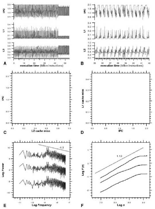
Figure 1: Execution traces for the program bzip2. (A) Evolution of the number of instructions executed per cycle (IPC), the rate of L1 cache misses (L1) and that of L2 cache misses (L2) during the first 54 billion instructions and (B) enlargement of the part comprised between 35 and 42 billion instructions. Also shown are projections of the dynamics attractor (C) in the IPC-L2 cache miss rate phase plan and (D) in the L1-IPC phase plan. The presence of long term correlations in these signals was sought for by Power Spectrum and Detrended Fluctuation Analysis (DFA). The power spectrum is presented in (E) as a log-log plot of the data concerning, from bottom to top, L1, L2 and IPC traces, respectively. The curves have been arbitrarily shifted along the y-axis to avoid overlap. Frequency is expressed in $instruction^{-1}$. The dashed line indicates a power-law decrease with exponent 1.3. The DFA graph (F) displays on a log-log scale the detrended fluctuations $F(n)$ as a function of the time scale $n$ (in instructions) for, from bottom to top, L1, L2 and IPC traces, respectively. Here, the dashed line indicate power-law growth with exponent 1.13. Note that the three DFA curves flatten when $n$ becomes higher than the major repetition period ($\approx 0.6$ billion instructions, see B).

IV Results

IV.1 First example: bzip2 time series

Figure 1 displays performance statistics for the program bzip2 acting on the source input of the ref data set (see II). We focus here on three statistics that are particularly relevant to computer performance: the number of instruction executed at each computer cycle (IPC), the instantaneous rate of L1 cache miss rate (L1) and that concerning L2 cache (L2). For readability, we only display in Figure 1A the traces obtained for the first 54 billion executed instructions (i.e. approximately one half of the total program execution). The three traces show two distinct phases: a first one with higher variability and lower frequency (up to circa 43 billion instructions), followed by a phase characterized by higher frequency and lower variability (from 43 to 54 billion instructions). Note that the second part of the total execution trace (not presented in Figure 1) essentially consists of a repetition of these two consecutive phases. In the remaining of this section we treat the entire ($\approx 110$ billion instruction long) trace as a single entity. Note however that we have also studied the two bzip2 execution phases separately (i.e. restraining the time series to the first phase, from 1 to 50 billion instructions, or to the second one, from 50 to 54 billion instructions) and obtained qualitatively similar results (though sensitivity to initial conditions seems higher in the second phase).

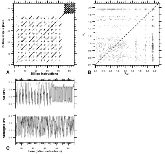
Figure 2: Study of the IPC trace for bzip2 after attractor reconstruction by embedding. (A) Recurrence plot corresponding to Figure 1A (thresholded at 0.136) (B) First return map for the Poincaré section at IPC minima. The dashed line indicates the first diagonal. (C) Surrogates data generated from the complete IPC trace. Shown are enlargements of the part comprised between 37 and 47 billion instructions of the original IPC time series (upper trace) and the corresponding surrogate trace (lower trace). Embedding parameters: delay $d=153$ million instructions, dimension $m=14$.

Although some regularity is readily seen in these time series, the two phases clearly display irregular or noisy dynamics. This is especially visible from the enlargement displayed Figure 1B. The dynamics present bounded and somewhat regular variations together with a large amount of variability. In particular, this figure evidences a major period of repetition of $\approx 0.6\times 10^{9}$ instructions. Figure 1C and D show projections of these dynamics in the IPC-L2 and L1-IPC phase plans. The resulting attractor projections display a characteristic mixture of regular structured zones together with ”cloudy” areas, hence confirming the high variability of the time series.
The observed variability could be imputed to a noise source (as part of the dynamics itself or resulting from the sampling method). Alternatively, it could be a direct result of deterministic chaotic dynamics. To discriminate between both possibilities, several tests are available in the time series analysis literature. These tests are usually individually conclusive when employed on long and perfect synthetic time series. Real world time series however, usually incorporate high levels of noise stemming from experimental measurements, and are often much smaller, so that conclusive decisions generally need the investigation of the results provided by several of these tests. Thus, several converging approaches are necessary to identify nonlinear patterns and avoid spurious determinations.
We first sought for long term correlations in the time series of Figure 1 using spectral and detrended fluctuation analysis (see III.1). Figure 1E shows the power spectrum $S(f)$ variations with the frequency $f$ on a log-log scale. First, we note that the power spectrum has a broadband characteristic, typical of stochastic and chaotic signals. Furthermore, for the three statistics tested, the power spectrum scales as a power-law of the frequency, for frequencies $f\gtrapprox 2\times 10^{-9}\quad instruction^{-1}$ (i.e. for periods lower than the major period of repetition) with spectral exponent $\beta\approx 1.3$. Detrended fluctuation analysis for the three time series is presented Figure 1F. Here again, for time scales lower than the major period of repetition, we observe for the three time series a power-law relationship between $F(n)$ and $n$, with an exponent $\alpha\approx 1.13$.

Figure 3: Characterization of the attractor for bzip2 after reconstruction by embedding of the IPC trace. (A) Log-log plot of the correlation sums $C(m,\epsilon)$ as a function of the considered neighborhood $\epsilon$, with $m$ ranging, from top to bottom, from $1$ to $25$ (with increment of 1). (B) Corresponding local slopes $d\ln C(m,\epsilon)/d\ln\epsilon$ with $m$ ranging, from top to bottom, from $25$ to $7$ (with decrement of 1). The dashed line indicates the value estimated for the correlation dimension $D_{2}=2.3\pm 0.3$ (C) Corresponding estimates of the correlation entropy $h_{2}$. The dashed line indicates the value 0.125, yielding $h_{2}\approx 1.2$ bits/billion instructions. (D) Estimation of the largest Lyapunov exponent (see  III.6) using the Rösenstein’s (bottom trace) or Kantz’s (top traces) method with $m=12$ to $15$ (from top to bottom). The dashed line indicates a power-law growth with exponent 0.42, yielding an estimate of $\lambda_{max}\approx 0.60$ bits/billion instructions. Embedding parameters are those of figure 2.

Note that the two independently-obtained exponent values satisfy the relationship $\alpha=(1+\beta)/2$ Buldyrev et al. (1995); Heneghan and McDarby (2000), which is an indication of the consistency of these values Rangarajan and Ding (2000).
These results first show that bzip2 performance statistics display $1/f^{\beta}$-noise. This reveals the absence of a characteristic time scale for the duration and recurrence of the performance variations (at least for those variations with time-scales shorter than the major period of repetition). Hence bzip2 performance time series display a high level of self-similarity. Furthermore, the value obtained for $\alpha$ is greater than 0.5 (and $\beta>1$). This is a sign of the existence of persistent long-range correlations inside the time series i.e. a large (compared to the average) IPC or cache miss rate value is more likely to be followed by a large IPC or cache miss rate value and vice versa. The presence of these correlations is a first argument to exclude the possibility of (noncorrelated) noise as a source of variability of the traces.
To study further the dynamics, we reconstructed its attractor through embedding of the IPC time series. The embedding parameters (delay $d$ and dimensions $m$ see III.2) were estimated to $d=153$ million instructions and $m=14$. Figure 2A presents the thresholded recurrence plot. We first note that the two consecutive phases displayed by bzip2 (see Figure 1A) are clearly recognizable from the recurrence plot, indicating that their recurrence rates may be significantly different. Interestingly, the plot presents many interrupted diagonal lines beside single isolated points. Furthermore, these lines exhibit some level of periodicity, which could be a sign that the system contains unstable periodic orbits (UPOs) Bradley and Mantilla (2002). This kind of structure is typical of chaotic systems Eckmann et al. (1987). We also present in Figure 2B the first-return map of the Poincaré section at IPC minima of the reconstructed attractor. The map is highly structured, with several mono-dimensional parts, which is another sign of low dimensional chaotic dynamics.
Thus, these first elements plead in favor of a chaotic component in bzip2 performance time series. Chaotic dynamics being a manifestation of nonlinear systems, we next sought the presence of nonlinearities in this time series using surrogates data (see III.7). Figure 2C shows a segment of the time series (upper trace) together with the corresponding surrogate (lower trace). Visual comparison of these two signals already suggests their dissimilarity. To confirm visual inspection, we performed statistical tests, quantifying nonlinearity with two different statistics. The null hypothesis was that the IPC trace could be generated by a linear, possibly rescaled, Gaussian random process. Both quantification statistics yield to reject the null hypothesis at the 95% level of significance, hence confirming the nonlinear nature of the IPC execution trace.
To study the reconstructed attractor in more details, we next characterized its geometrical properties. Figure 3A displays a log-log plot of the correlation sums $C(m,\epsilon)$ obtained for various dimensions $m$, versus the neighborhood size $\epsilon$. A power-law regime between $\epsilon\approx 0.02$ and $\epsilon\approx 0.3$ is apparent for high $m$ values. Furthermore, the corresponding slopes in this regime (the exponents of the power-laws) seem to tend to a rather constant value at high $m$. This scaling is confirmed in Figure 3B that shows the local slopes $d\ln C(m,\epsilon)/d\ln\epsilon$ of the curves of Figure 3A. For $0.03\lessapprox\epsilon\lessapprox 0.3$ and $m\gtrapprox 9$, the local slopes collapse to a $m$- and $\epsilon$-independent value of $\approx 2.3$. The occurrence of such a scaling regime is a strong sign that the observed variability in the dynamics is not caused by a random source, thus confirming the hypothesis of a chaotic behavior. The value in the scaling regime is an estimation of the correlation dimension of the attractor, $D_{2}=2.3\pm 0.3$. The correlation dimension is one measure of the attractor fractality. Thus, its non-integer value might be an indication that the attractor for bzip2 performance dynamics is a fractal object, like most of the chaotic strange attractors. However, as is very often the case with real-life systems, our estimation of $D_{2}$ is not precise enough to exclude an integer value, so that the attractor fractality cannot be asserted in the light of our present results. However, the (low) value of $D_{2}$ remains a strong indication the bzip2 performance displays low-dimensional chaos.

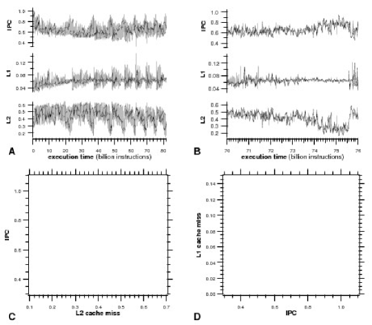
Figure 4: Execution traces for the program vpr. (A) Evolution of the number of instructions executed per cycle (IPC), the rate of L1 cache misses (L1) and that of L2 cache misses (L2) over the complete program execution and (B) enlargement of the segment comprised between 70 and 76 billion instructions. Also shown are projections of the dynamics attractor (C) in the IPC-L2 cache miss rate phase plan and (D) in the L1-IPC phase plan.

The correlation sums can also be used to estimate the corresponding correlation entropy $h_{2}$. Figure 3C presents the resulting estimates as a function of $\epsilon$ and for $m$ varying from 7 to 25. The value of $h_{2}$ can be estimated in the scaling regime observed in Figure 3B, but must be extrapolated at large $m$. Accordingly, our estimate on the basis of Figure 3C (dashed line) yields $h_{2}\approx 1.2$ bits/billion instructions.
A very strong indication of chaotic dynamics is sensitivity to initial conditions (SCI). To quantify SCI in our systems, we tried to estimate the largest Lyapunov exponent from our reconstructed attractor (Figure 3C) using both Kantz’s Kantz (1994) (top four curves) and Rösenstein’sRosenstein et al. (1993) (bottom curve) methods. The occurrence of a positive Lyapunov exponent is amongst the strongest indications of chaotic dynamics. Both methods result in similar curve shapes. Although the data are far from ideal, a linear part at short times can be distinguished in all these curves. The slope of these linear parts provides us with an estimate for the largest Lyapunov exponent $\lambda_{max}\approx 0.60$ bits/billion instructions. Alternatively, the largest Lyapunov exponent can also be measured from the Poincaré map. Our estimations on the basis of Figure 2B (data not shown) yield a somewhat higher, but comparable estimate ($\lambda_{max}\approx 1.22$ bits/billion instructions). These estimates can be compared to the correlation entropy $h_{2}$, which is a lower bound of the sum of all the positive Lyapunov exponents of the system (see III.5). Hence our estimates for $h_{2}$ and $\lambda_{max}$ are readily comparable, thereby further supporting the consistency of our measurements.
The measurements and analysis presented so far were essentially obtained on the basis of a reconstruction of the attractor using the IPC time series. We also carried out most of these analyzes using the other two time series (L2 and L1 cache miss rates) for attractor reconstruction and varied the averaging window $\tau_{av}$ ($\tau_{av}=10^{6},\,10^{7}\,\mathrm{or}\,10^{8}$ instructions, see II). All these conditions yielded comparable values and confirmed that bzip2 performance dynamics display low dimensional deterministic chaos. Furthermore, we analyzed bzip2 performance dynamics with another data input (namely, the program input of the ref data set, see  II). Although these dynamics displayed possibly lower SCI ($\lambda_{max}\approx 0.5$ bits/billion instructions), all tested indicators confirmed the presence of chaotic dynamics, indicating that their origin is more probably rooted into the program/architecture interaction than to be found in a data-dependent mechanism.

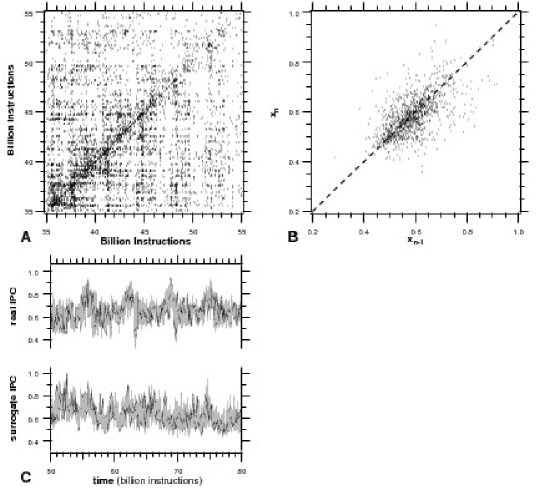
Figure 5: Study of the IPC trace for vpr after attractor reconstruction by embedding. (A) Recurrence plot thresholded at 0.079. Note that, for readability, we only present the data obtained for the segment ranging from 35 to 55 billion instructions. (B) First return map for the Poincaré section at IPC minima. The dashed line indicates the first diagonal. (C) Surrogates data developed from the complete IPC trace. Shown are enlargements of the part comprised between 50 and 80 billion instructions of the original IPC time series (upper trace) and corresponding surrogate trace (lower trace). Embedding parameters: delay $d=350$ million instructions, dimension $m=5$.

The magnitude of the largest Lyapunov exponent quantifies the attractor’s dynamics in information theoretic terms. As a crude interpretation, it measures the rate at which the system destroys information. For instance, suppose one knows the number of instruction executed per cycle for bzip2 at some initial time $t_{0}$ with good accuracy, say $0.01\%$ (13 bits). Because of the intrinsic sensitivity to initial conditions (say, in average, $\lambda_{max}\approx 0.9$ bits/$10^{9}$ instructions), 0.9 bits of this information will be lost, in average, every billion instructions. In other words, after 15 billion instructions (i.e. $\approx 1/8$ of the total program execution length), the IPC number would be no more predictable. Note however that the magnitudes of the Lyapunov exponents quantify average convergence or divergence rates (over the phase space), but in fact, the degree of predictability can vary considerably throughout phase space Abarbanel et al. (1991). Hence it is possible to loose predictability exponentially fast in some part of the dynamics, while regaining it later on.
To compare with other chaotic systems, these values must be related to the duration of an average orbit around the attractor, which is $\approx 430$ million instructions, yielding a value ranging from 0.26 to 0.52 bits/average orbit. Although lower than that of the Lorenz system ($\lambda_{max}=1.36$ bits/orbits), this value is comparable to that obtained for the Rössler system ($\lambda_{max}=0.78$ bits/orbits) Wolf et al. (1985), a classical model for deterministic chaos.
Finally, we note that this kind of dynamics is not restricted to bzip2. Amongst the tested Spec benchmarks, we evidenced deterministic chaos with other programs including galgel and fma3d, and obtained some indications of it (albeit not conclusively) for gzip and ammp.

Figure 6: Characterization of the attractor for vpr after reconstruction by embedding of the IPC trace. (A) Log-log plot of the correlation sums $C(m,\epsilon)$ as a function of the considered neighborhood $\epsilon$, with $m$ ranging, from top to bottom, from $1$ to $20$ (with increment of 1). (B) Corresponding local slopes $d\ln C(m,\epsilon)/d\ln\epsilon$ with $m$ ranging, from top to bottom, from $20$ to $1$ (with increment of 1). Embedding parameters are those of figure 5.

IV.2 Second example: vpr time series

Evolution of the three studied performance statistics for the program vpr are shown Figure 4. As compared to bzip2, the dynamics are much more variable and lack real regular behaviors. Likewise, the projections onto phase plans display clouds of points lacking clear inner structures. We reconstructed the attractor of the dynamics through embedding of the IPC time series (with $d=350$ million instructions and $m=5$).
Figure 5A presents the thresholded recurrence plot for this embedding. In opposition to the recurrence plot obtained for bzip2 (Figure 2A), vpr recurrence plot only displays isolated points (no diagonal lines) that are much more homogeneously distributed (distribution structures are not easily visible). Likewise, the Poincaré map presented Figure 5B displays a rather homogeneous scattering of the points over the first diagonal. The aspect of these two figures are first indications that vpr variability is neither periodic, nor the result of chaotic dynamics. In agreement with these conclusions, we note that, even if the corresponding surrogates (Figure 5C) are visually similar to the original IPC time series, statistical tests for the presence of nonlinearities in vpr performance dynamics could not decide between the presence or the absence of nonlinearity in the original trace. This can be considered as a first indication that, while not chaotic nor periodic, this time series might neither result from a really stochastic process.

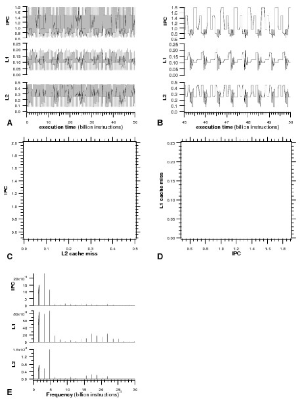
Figure 7: Execution traces for the program applu. (A) Evolution of the number of instructions executed per cycle (IPC), the rate of L1 cache misses (L1) and that of L2 cache misses (L2) over the first 50 billion instructions (the entire program execution consists of circa 220 billion instructions) and (B) enlargement of the segment comprised between 45 and 50 billion instructions. Also shown are projections of the dynamics attractor (C) in the IPC-L2 cache miss rate phase plan and (D) in the L1-IPC phase plan. The power spectra for the three time series are presented in (E)

Figure 6 shows the corresponding correlation sums for $m$ ranging (from top to bottom) from 1 to 20. Although a regime with power-law behavior is observed for each curve, the slopes of the corresponding linear parts do not seem to saturate to a constant value with increasing $m$. This is confirmed by examination of the respective local slopes presented Figure 6B. In opposition to the corresponding plot for bzip2 (Figure 3B), this figure fails to show any scaling regime, whatever the $\epsilon$- or $m$-range considered. Absence of saturation of the correlation sum exponents at high $m$ is another indication that, contrarily to bzip2, the high variability and irregularity of vpr performance dynamics are not imputable to chaotic dynamics, but result from some “high dimensional” non chaotic process.
Amongst the Spec benchmarks we inspected, a similar behavior was also observed for art, and suspected for several other programs, such as crafty, and (albeit to a lesser extend) ammp, gcc, or gzip.

IV.3 Third example: applu time series

Our last example concerns the program applu, a scientific computing application. A simple inspection of the time series is enough to evidence the regularity of the three performance statistics (Figure 7A and B). Projections in the phase plans (Figure 7C and D) provide a striking representation of a multiply folded one-dimensional attractor, reminiscent of multi-dimensional limit cycles. These periodic oscillations are so regular that the folded attractors display an almost null noise level. In agreement with these observations the power spectra for the three statistics (Figure 7E) are typical of periodic patterns, with a major frequency ($f\approx 1.6\times 10^{-9}$ instructions corresponding to a period of $\approx 0.6$ billion instructions, compare with Figure 7B) and its harmonics dominating the spectrum.
Taken together, these results unambiguously show the existence of programs with highly regular performance traces. Besides applu, such a behavior was also evidenced for other Spec benchmark programs such as apsi.

V Discussion

V.1 Potential sources of seemingly stochastic dynamics

An intriguing result of this paper is that the performance traces of several program are not periodic nor chaotic, but display a high level of aperiodic fluctuations (such as vpr), that appear similar to stochastic dynamics from the point of view of the nonlinear methods we used. This may sound counterintuitive because the underlying microprocessor operations are deterministic by nature. Several sources of aperiodic variability in the performances can be evoked.
First, a potential source of aperiodicity resides in the simulated programs themselves. A great number of the programs from the SPEC benchmark are scientific codes and many of them use pseudo-random numbers. Albeit pseudo-random number generators are also purely deterministic routines, their output is hardly distinguishable from truly random numbers. This could in part be implied in the apparently stochastic behaviors we observed. Second, one must not forget that the metrics we studied are indirect measurements of the microprocessor state. In other words, while the microprocessor deterministically processes the program flow, we only record its performance. It has recently been remarked that the correlation between the code being executed and the performance can vary widely Annavaram et al. (2004). In other words, for some programs, performance metrics are highly dependent on the execution history, so that two executions of the same code piece during a single program can have performance metrics that vary considerably. This source of variability could also in part explain the behavior of “high dimensional” traces such as vpr.
Furthermore, recall that to distinguish between chaotic and stochastic signals, nonlinear time series methods usually make use of the fact that, contrarily to stochastic dynamics, chaotic ones are “bounded” (their attractor have a finite dimension). In the same way that these methods could not distinguish purely random numbers from pseudo-random numbers generated by modern libraries, the vpr traces could abusively appear stochastic to them. In fact, even simple deterministic processes can yield behaviors that appear stochastic to visual inspections (see for example Chapter 4 in Wolfram (2002)). Incidentally, we note that the IPC time series of vpr is strikingly similar to the apparently stochastic fluctuations of the simple deterministic recursive iteration presented page 130 (bottom trace) in Wolfram (2002). Hence, what can rigorously be said of the vpr case is that it is highly fluctuating, and that these fluctuations are neither regular (periodic) nor chaotic, but result of a “high dimensional” process.

V.2 Chaotic performance time series and predictability

The other specific conclusion drawn by this study is that the high variability in the time-evolution of the performances during the execution of several programs can be imputed to deterministic chaos. This result seems important because it implies that performance predictability based on short sampled sequences might be impossible and because in a more general perspective, it reveals the high intricacy of the processes determining instantaneous microprocessor performances. However, its interpretation must be handled with great care. First, the obtained results apply to instantaneous performances only and do not imply other aspects of microprocessor operations. For instance, they neither imply that program execution itself (i.e. the instruction flow handled by the processor) is chaotic or unpredictable. In particular, they do not imply that the program final result might be variable nor unpredictable.
Chaotic dynamics are known to occur in systems where the variables are in great number and/or interact through nonlinear relationships. Modern microprocessors include a large number of hardware mechanisms that are dedicated to improve performance (speculative execution, branch predictors, prefetchers, memory and instruction caches, pipelines…). As a result, the precise number of cycles needed to execute a given instruction sequence depends on a huge number of internal states of hardware components. For instance, the precise number of clock cycles needed to execute a simple instruction sequence including at least one conditional branch and one load/store instruction depends, among others, on the state of the branch predictor mechanism (which is usually history-dependent) corresponding to this branch, on the states of the different caches of the memory hierarchy (presence or absence of the data), the precise state of all instructions in all stages of the execution pipeline and in the numerous buffers included in the processors. Furthermore, these different internal states are usually related through nonlinear relationships (for instance, a branch prediction error can lead to a complete flush of the execution pipeline, which may, in turn modify this branch predictor state).
Hence, exact knowledge of the state of the set of performance-determining mechanisms at a given time is unattainable. This property is so strong that it has recently been used to build powerful pseudo-random number generators based on the unpredictability of the internal microprocessor states Seznec and Sendrier (2003). As a result, two states of the performance-determining mechanisms that appear arbitrarily close with respect to the partial information possessed by the observer, can in fact be different. Because performance critically depends on the global state, the performance evolutions starting from these two seemingly similar states can be highly different. This might account for the observed sensitivity to initial conditions (i.e. chaos). Note however that further work is needed to understand why these properties manifest during the execution of certain programs only, while it seems not to be prominent for others.

V.3 Relevance to practical applications

Finally our results may have some practical importance in the field of performance modeling. To predict the effect of a given hardware mechanism, computer architects use detailed simulations of the microprocessor performance during program execution. Because these detailed simulations are highly demanding on calculation time, several methods have been developed to estimate the average performance on the basis of a subsample of the entire execution trace. Our result that several program traces (such as vpr) display dynamics that are closed to stochastic ones could be useful in this framework. Indeed, this usually means that the obtained surrogates data are very similar to the corresponding real traces (see figure 5C, for instance). Hence, for these programs, it is possible to consider generating long surrogates data (at very low computational costs) from a short sample of the real trace, and use these synthetic traces to estimate the average metric (average ipc, for example) during a real execution of the program.
Conversely, our results indicate that for those programs endowed with chaotic behaviors (such as bzip2 or galgel), it might be very delicate to predict the actual evolution of the considered performance metric on the basis of extrapolations from a short sequence of the real trace. Hence, for these programs, our results suggest that an efficient strategy for predicting the actual average value of the metric under consideration on the ground of a sample of its real trace would be to base the estimation on several samples extracted from the real trace, even in a random way. Actually this method is used by one of the most powerful tool developed for performance prediction Wunderlich et al. (2003). Yet, it should be recalled that variations on a strange attractor are bounded so that the existence of these difficulties does not exclude the possibility to predict accurate average values, which is the aim of most of these methods Sherwood et al. (2002); Perelman et al. (2003). Finally, the necessity to adapt the performance simulation/sampling technique as a function of the program under consideration has recently been pointed out Annavaram et al. (2004). We think our results might account for a rationale of this necessity.

References

- Moore (1965) G. E. Moore, Electronics 38 (1965).
- Stephenson and Amarasinghe (2005) M. Stephenson and S. Amarasinghe, in Proc. International Symposium on Code Generation and Optimization (CGO) (2005).
- Kulkarni et al. (2004) P. Kulkarni, S. Hines, J. Hiser, D. Whalley, J. Davidson, and D. Jones, in Proc. ACM SIGPLAN Conference on Programming Language Design and Implementation (PLDI) (2004).
- Fursin et al. (2002) G. Fursin, M. O’Boyle, and P. Knijnenburg, in Proc. Languages and Compilers for Parallel Computers (LCPC) (2002), pp. 305–315.
- Duesterwald et al. (2003) E. Duesterwald, C. Cascaval, and S. Dwarkadas, in Proc. 12th International Conference on Parallel Architectures and Compilation Techniques (PACT’03) (New Orleans, Louisiana, 2003), pp. 220–231.
- Annavaram et al. (2004) M. Annavaram, R. Rakvic, M. Polito, J.-Y. Bouguet, R. Hankins, and B. Davies, in Proc. 37th annual IEEE ACM International Symposium on Microarchitecture (MICRO-37) (Portland, OR, 2004), pp. 93–104.
- Slingerland and Smith (2001) N. T. Slingerland and A. J. Smith, in ICS ’01: Proceedings of the 15th international conference on Supercomputing (ACM Press, New York, NY, USA, 2001), pp. 204–217, ISBN 1-58113-410-X.
- Lam et al. (1991) M. D. Lam, E. E. Rothberg, and M. E. Wolf, in ASPLOS-IV: Proceedings of the fourth international conference on Architectural support for programming languages and operating systems (ACM Press, New York, NY, USA, 1991), pp. 63–74, ISBN 0-89791-380-9.
- Coleman and McKinley (1995) S. Coleman and K. McKinley, in Proc. PLDI (1995), pp. 279–290.
- Gluhovsky and O’Krafka (2005) I. Gluhovsky and B. O’Krafka, ACM Trans. Comput. Syst. 23, 111 (2005), ISSN 0734-2071.
- Abella et al. (2001) J. Abella, A. Gonzalez, J. Llosa, and X. Vera, Near-optimal loop tiling by means of cache miss equations and genetic algorithms (2001), URL citeseer.csail.mit.edu/abella01nearoptimal.html.
- Burger et al. (1996) D. Burger, T. M. Austin, and S. Bennett, Tech. Rep. CS-TR-1996-1308 (1996), URL citeseer.ist.psu.edu/burger96evaluating.html.
- Karkhanis and Smith (2004) T. S. Karkhanis and J. E. Smith, in ISCA ’04: Proceedings of the 31st annual international symposium on Computer architecture (IEEE Computer Society, Washington, DC, USA, 2004), p. 338, ISBN 0-7695-2143-6.
- Burger et al. (2004) D. Burger, T. M. Austin, and S. W. Keckler, SIGMETRICS Perform. Eval. Rev. 31, 4 (2004), ISSN 0163-5999.
- Koiran et al. (1994) P. Koiran, M. Cosnard, and M. H. Garzon, Theor. Comput. Sci. 132, 113 (1994).
- Cook (2004) M. Cook, Complex Systems 15, 1 (2004).
- Kilian and Siegelmann (1993) J. Kilian and H. Siegelmann, in Proceedings of the sixth annual ACM conference on computational learning theory (Santa Cruz, CA, USA, 1993).
- Siegelmann and Sontag (1991) H. Siegelmann and E. Sontag, Appl. Math. Lett 4, 77 (1991).
- Branicky (1995) M. Branicky, Theor. Comput. Sci. 138, 67 (1995).
- Omohundro (1984) S. Omohundro, Physica D 10, 128 (1984).
- Ŝíma and Orponen (2003) J. Ŝíma and P. Orponen, Neural Comput. 15, 693 (2003).
- Hegger et al. (1999) R. Hegger, H. Kantz, and T. Schreiber, CHAOS 9, 413 (1999).
- Schreiber (1999) T. Schreiber, Phys. Rep. 308, 2 (1999).
- Yamamoto (1999) Y. Yamamoto, Modern techniques in neuroscience research (Springer-Verlag, Berlin, 1999), chap. Detection of chaos and fractals from experimental time series, pp. 669–687.
- Peng et al. (1995) C.-K. Peng, S. Havlin, H. Stanley, and A. Goldberger, CHAOS 5, 82 (1995).
- Rangarajan and Ding (2000) G. Rangarajan and M. Ding, Phys. Rev. E 61, 4991 (2000).
- Takens (1981) F. Takens, in Dynamical Systems and Turbulence, edited by D. Rand and L.-S. Young (Springer-Verlag, 1981), vol. 898 of Lecture Notes in Math., pp. 366–381.
- Packard et al. (1980) N. Packard, J. P. Crutchfield, J. D. Farmer, and R. S. Shaw, Phys. Rev. Lett. 45, 712 (1980).
- Casdagli et al. (1991) M. Casdagli, S. Eubank, J. D. Farmer, and J. Gibson, Physica D 51, 52 (1991).
- Rosenstein et al. (1993) M. Rosenstein, J. Collins, and C. D. Luca, Physica D 65, 117 (1993).
- Abarbanel (1996) H. Abarbanel, Analysis of observed chaotic data (Springer-Verlag, New-York, 1996).
- Kantz and Schreiber (1996) H. Kantz and T. Schreiber, Nonlinear time series analysis (Cambridge University Press, Cambridge, 1996).
- Kennel et al. (1992) M. Kennel, R. Brown, and H. Abarbanel, Phys. Rev. A 45, 3403 (1992).
- Eckmann et al. (1987) J.-P. Eckmann, S. O. Kamphorst, and D. Ruelle, Europhysics Letters 5, 973 (1987).
- Zbilut et al. (2002) J. Zbilut, N. Thomasson, and C. Webber, Med. Eng. Phys. 24, 53 (2002).
- Thiel et al. (2004) M. Thiel, M. Romano, J. Kurths, and P. Read, CHAOS 14, 234 (2004).
- Theiler (1990) J. Theiler, J. Opt. Soc. Am. A 7, 1055 (1990).
- Kantz (1994) H. Kantz, Phys. Lett. A 185, 177 (1994).
- Schreiber and Schmitz (2000) T. Schreiber and A. Schmitz, Physica D 142, 346 (2000).
- Buldyrev et al. (1995) S. V. Buldyrev, A. L. Goldberger, S. Havlin, R. N. Mantegna, M. E. Matsa, C.-K. Peng, M. Simons, and H. E. Stanley, Phys. Rev. E 51, 5084 (1995).
- Heneghan and McDarby (2000) C. Heneghan and G. McDarby, Phys. Rev. E 62, 6103 (2000).
- Bradley and Mantilla (2002) E. Bradley and R. Mantilla, CHAOS 12, 596 (2002).
- Abarbanel et al. (1991) H. D. I. Abarbanel, R. Brown, and M. B. Kennel, J. Nonlinear Sci. 1, 175 (1991).
- Wolf et al. (1985) A. Wolf, J. Swift, H. Swinney, and J. Vastano, Physica D 16, 285 (1985).
- Wolfram (2002) S. Wolfram, A New Kind of Science (Wolfram Media, 2002), URL http://www.wolframscience.com.
- Seznec and Sendrier (2003) A. Seznec and N. Sendrier, ACM Transactions Modeling Computer Simulation 13, 334 (2003).
- Wunderlich et al. (2003) R. E. Wunderlich, T. F. Wenisch, B. Falsafi, and J. C. Hoe, in ISCA ’03: Proceedings of the 30th annual international symposium on Computer architecture (ACM Press, 2003), pp. 84–97, ISBN 0-7695-1945-8.
- Sherwood et al. (2002) T. Sherwood, E. Perelman, G. Hamerly, and B. Calder, SIGOPS Oper. Syst. Rev. 36, 45 (2002), ISSN 0163-5980.
- Perelman et al. (2003) E. Perelman, G. Hamerly, M. V. Biesbrouck, T. Sherwood, and B. Calder, in ACM SIGMETRICS the International Conference on Measurement and Modeling of Computer Systems (2003).