Generalized synchronization: a modified system approach

Abstract

The universal mechanism resulting in the generalized synchronization regime arising in the chaotic oscillators with the dissipative coupling has been described. The reasons of the generalized synchronization occurrence may be clarified by means of a modified system approach. The main results are illustrated by unidirectionally coupled Rössler systems, Rössler and Lorenz systems and logistic maps.

Chaotic synchronization is one of the fundamental phenomena, widely studied recently A. Pikovsky, M. Rosenblum, J. Kurths (2001), having both theoretical and applied significance (e.g., for information transmission by means of deterministic chaotic signals K. Murali, M. Lakshmanan (1994); T. Yang, C.W. Wu and L.O. Chua (1997), in biological and physiological L. Glass (2001) tasks, etc.). Several different types of chaotic synchronization of coupled oscillators, i.e. generalized synchronization (GS) P. Paoli, A. Politi, R. Badii (1989); N.F. Rulkov, M.M. Sushchik, L.S. Tsimring, H.D.I. Abarbanel (1995), phase synchronization (PS) A. Pikovsky, M. Rosenblum, J. Kurths (2001), lag synchronization (LS) M.G. Rosenblum, A.S. Pikovsky, J. Kurths (1997) and complete synchronization (CS) L.M. Pecora, T.L. Carroll (1990) are well known. There are also attempts to find unifying framework for chaotic synchronization of coupled dynamical systems R. Brown, L. Kocarev (2000); S. Boccaletti, J. Kurths, G. Osipov, D.L. Valladares, C.S. Zhou (2002); S. Boccaletti, L.M. Pecora, A. Pelaez (2001); A.E. Hramov, A.A. Koronovskii (2004).

One of the interesting and intricate types of the synchronous behavior of unidirectionally coupled chaotic oscillators is the generalized synchronization. The presence of GS between the response $\mathbf{x}_{r}(t)$ and drive $\mathbf{x}_{d}(t)$ chaotic systems means that there is some functional relation ${\mathbf{x}_{r}(t)=\mathbf{F}[\mathbf{x}_{d}(t)]}$ between system states after the transient finished. This functional relation $\mathbf{F}[\cdot]$ may be smooth or fractal. According to the properties of this relation, GS may be divided into the strong synchronization and week synchronization, respectively K. Pyragas (1996). There are several methods to detect the presence of GS between chaotic oscillators, such as the auxiliary system approach H.D.I. Abarbanel, N.F. Rulkov, M.M. Sushchik (1996) or the method of nearest neighbors N.F. Rulkov, M.M. Sushchik, L.S. Tsimring, H.D.I. Abarbanel (1995); L.M. Pecora, T.L. Carroll, J.F. Heagy (1995). It is also possible to calculate the conditional Lyapunov exponents (CLEs) L.M. Pecora, T.L. Carroll (1991); K. Pyragas (1996) to detect GS. The regimes of LS and CS are also the particular cases of GS.

This paper aims to explain GS arising. We show the physical reasons leading to GS appearance in unidirectionally coupled chaotic systems. The causes of the generalized synchronization arising may be clarified by means of a modified system approach.

Let us consider the behavior of two unidirectionally coupled chaotic oscillators

$$\begin{split}&\mathbf{\dot{x}}_{d}=\mathbf{H}(\mathbf{x}_{d},\mathbf{g}_{d})\\ &\mathbf{\dot{x}}_{r}=\mathbf{G}(\mathbf{x}_{r},\mathbf{g}_{r})+\varepsilon\mathbf{P}(\mathbf{x}_{d},\mathbf{x}_{r}),\\ \end{split}$$ (1)

where $\mathbf{x}_{d,r}$ are the state vectors of the drive and response systems, respectively; $\mathbf{H}$ and $\mathbf{G}$ define the vector fields of these systems, $\mathbf{g}_{d}$ and $\mathbf{g}_{r}$ are the controlling parameter vectors, $\mathbf{P}$ denotes the coupling term and $\varepsilon$ is the scalar coupling parameter. If the dimensions of the drive and response systems are $N_{d}$ and $N_{r}$ respectively, the behavior of the unidirectionally coupled oscillators (1) is characterized by the Lyapunov exponent (LEs) spectrum ${\lambda_{1}\geq\lambda_{2}\geq\dots\geq\lambda_{N_{d}+N_{r}}}$. Due to the independence of the drive system dynamics on the behavior of the response one, the Lyapunov exponent spectrum may be divided into two parts: LEs of the drive system ${\lambda^{d}_{1}\geq\dots\geq\lambda^{d}_{N_{d}}}$ and the CLEs L.M. Pecora, T.L. Carroll (1991); K. Pyragas (1997) ${\lambda^{r}_{1}\geq\dots\geq\lambda^{r}_{N_{r}}}$. The condition of GS is $\lambda^{r}_{1}<0$ (see K. Pyragas (1996) for detail).

The GS manifestation is mostly considered for two identical systems with equal or mismatched parameters and diffusive type of unidirectional coupling. Therefore, let us consider such systems first, while the case of different systems and others coupling types will be briefly discussed later. In the case of identical systems the dimensions of the drive and response oscillators are equal ($N_{d}=N_{r}=N$) and the equations (1) may be rewritten as

$$\begin{split}&\mathbf{\dot{x}}_{d}=\mathbf{H}(\mathbf{x}_{d},\mathbf{g}_{d})\\ &\mathbf{\dot{x}}_{r}=\mathbf{H}(\mathbf{x}_{r},\mathbf{g}_{r})+\varepsilon\mathbf{A}(\mathbf{x}_{d}-\mathbf{x}_{r}),\end{split}$$ (2)

where $\mathbf{A}={\{\delta_{ij}\}}$ is the coupling matrix, $\delta_{ii}=0$ or $1$ and $\delta_{ij}=0$ ($i\neq j$). It is clear, that the dynamics of the response system may be considered as the non-autonomous dynamics of the modified system

$$\mathbf{\dot{x}}_{m}=\mathbf{H}^{\prime}(\mathbf{x}_{m},\mathbf{g}_{r},\varepsilon)$$ (3)

under the external force $\varepsilon\mathbf{A}\mathbf{x}_{d}$

$$\mathbf{\dot{x}}_{m}=\mathbf{H}^{\prime}(\mathbf{x}_{m},\mathbf{g}_{r},\varepsilon)+\varepsilon\mathbf{A}\mathbf{x}_{d},$$ (4)

where $\mathbf{H}^{\prime}(\mathbf{x},\mathbf{g})=\mathbf{H}(\mathbf{x},\mathbf{g})-\varepsilon\mathbf{A}\mathbf{x}$. Note, that the term $-\varepsilon\mathbf{A}\mathbf{x}$ brings the dissipation into the modified system (3).

So, GS arising in (2) with parameter $\varepsilon$ increasing may be considered as a result of two cooperative processes taking place simultaneously. The first of them is the growth of the dissipation in the system (3) and the second one is the increasing of the amplitude of the external signal. Both processes are correlated with each other by means of the parameter $\varepsilon$ and can not be realized in the coupled oscillators system (2) independently. Nevertheless, let us consider these processes separately to understand better the mechanisms of GS arising. We start our considering with the autonomous dynamics of the modified system (3).

For this modified system, $\mathbf{x}_{m}(t)$, the quantity $\varepsilon$ is the dissipation parameter. When $\varepsilon$ is equal to zero the dynamics of the modified system $\mathbf{x}_{m}(t)$ coincides with the response system $\mathbf{x}_{r}(t)$ without coupling. With increasing of the dissipation parameter $\varepsilon$ the dynamics of the modified system (3) should be simplified. Therefore, the system $\mathbf{x}_{m}(t)$ has to undergo a transition from chaotic oscillations to periodic ones, and, perhaps, to the stationary state (if the dissipation is large enough). In this case one of the Lyapunov exponent, $\lambda_{0}^{m}$, of the modified system is equal to zero (or negative if the stationary state takes place), all other Lyapunov exponents are negative (${0>\lambda^{m}_{1}\geq\dots\geq\lambda^{m}_{N-1}}$). It is important to note, that the Lyapunov exponent spectrum of the modified system (3) differs from CLE spectrum ${\lambda^{r}_{1}\geq\dots\geq\lambda^{r}_{N}}$ of the system (2), as CLEs depend on the drive system dynamics in contrast to Lyapunov exponents of the modified system $\mathbf{x}_{m}(t)$. Therefore, nobody can draw a conclusion about the appearance of GS in the coupled oscillators system (2) taking into account only Lyapunov exponents of the modified system (3).

On the contrary, the external signal in (4) tends to impose the dynamics of the drive chaotic oscillator $\mathbf{x}_{d}(t)$ on the modified system $\mathbf{x}_{m}(t)$, and, correspondingly, complicate its dynamics. Obviously, GS may take place only if proper chaotic dynamics of the system $\mathbf{x}_{m}(t)$ is suppressed by the dissipation. Only under this condition the current state $\mathbf{x}_{m}(t)$ of the modified system will be determined completely by the external signal, i.e. $\mathbf{x}_{m}(t)=\mathbf{F}[\mathbf{x}_{d}(t)]$. According to the equation (4), the functional relation $\mathbf{x}_{r}(t)=\mathbf{F}[\mathbf{x}_{d}(t)]$ between the response and drive systems will also take place, and, therefore, GS will be observed.

So, GS arising in the system (2) is possible for such values of $\varepsilon$ parameter when the modified system $\mathbf{x}_{m}(t)$ demonstrates the periodic oscillations or the stationary state. It is well known, that even the harmonic external signal can cause the chaotic oscillations in the dynamical system with periodical dynamics. Therefore, the periodic regime should be stable enough for the external force not to excite proper chaotic dynamics of the modified system. So, the difference between the parameter values $\varepsilon_{p}$ when the periodic oscillations take place in the system (3) and $\varepsilon_{GS}$ when GS in the system (2) can be observed has to be large enough. At the same time, the amplitude of the external signal is small enough in comparison with the amplitude of periodic oscillations in the modified system $\mathbf{x}_{m}(t)$ (in the case when the periodical regime takes place in (3)). So, the generalized synchronization looks like the week chaotic excitation of the periodical motion.

The similar conclusion is also correct for the stationary regime of the system $\mathbf{x}_{m}(t)$ when GS manifests itself as chaotic perturbation of the fixed state. The system dynamics can be considered as transient converging to the “fixed” point moving under the external force in the phase space of the modified system (3). Let us suppose now that controlling parameters $\mathbf{g}_{r,d}$ of the considered response and drive systems differ from each other slightly and the value of parameter $\varepsilon$ is large enough. In this case the transient is very short and the state of the modified system follows the perturbed “fixed” state essentially small time $\tau$ of delay, therefore the regime of LS can be observed.

Let us consider several examples of GS to illustrate the concept described above. As the first system we have selected two unidirectionally coupled Rössler oscillators

$$\begin{array}[]{l}\dot{x}_{d}=-\omega_{d}y_{d}-z_{d},\\ \dot{y}_{d}=\omega_{d}x_{d}+ay_{d},\\ \dot{z}_{d}=p+z_{d}(x_{d}-c),\\ \\ \dot{x}_{r}=-\omega_{r}y_{r}-z_{r}+\varepsilon(x_{d}-x_{r}),\\ \dot{y}_{r}=\omega_{r}x_{r}+ay_{r},\\ \dot{z}_{r}=p+z_{r}(x_{r}-c),\end{array}$$ (5)

where $\varepsilon$ is a coupling parameter, $\omega_{r}=0.95$. The control parameter values have been selected by analogy with Z. Zheng, G. Hu (2000) as $a=0.15$, $p=0.2$, $c=10.0$. Correspondingly, the modified Rössler system is

$$\begin{array}[]{l}\dot{x}_{m}=-\omega_{r}y_{m}-z_{m}-\varepsilon x_{m},\\ \dot{y}_{m}=\omega_{r}x_{m}+ay_{m},\\ \dot{z}_{m}=p+z_{m}(x_{m}-c).\end{array}$$ (6)

In Fig 1,a the bifurcation diagram for the system (6) is shown. It is clear that this system undergoes the transition from chaotic to periodic oscillations through the inverse cascade of period doubling. The dependence of two largest Lyapunov exponents $\lambda^{m}_{0,1}$ on the parameter $\varepsilon$ is presented in Fig. 1,b. One can easily see, that starting from the value $\varepsilon_{p}\approx 0.06$ the periodic oscillations take place in the modified system (6).

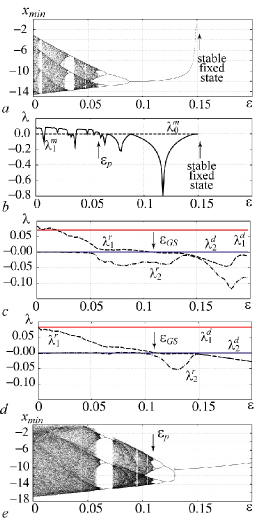
Figure 1: The bifurcation diagram (a) and the dependence of two Lyapunov exponent $\lambda^{m}_{0,1}$ (b) of the modified Rössler system (6) on the parameter $\varepsilon$. The third Lyapunov exponent is about $\lambda^{m}_{2}\approx-9.7$ and is not significant for our considering. The value of parameter $\varepsilon_{p}$ when the modified system starts demonstrating the periodic dynamics is shown by an arrow. (c,d) The dependence of the Lyapunov exponent spectrum on the parameter $\varepsilon$ for slightly ($\omega_{d}=0.99$) and greatly ($\omega_{d}=1.3$) detuned Rössler systems, respectively. The onset of GS is marked by an arrow. Conditional Lyapunov exponents are presented by dashed ($\lambda^{r}_{1}$) and dotted ($\lambda^{r}_{2}$) lines. (e) The bifurcation diagram for the non-autonomous modified system. The first equation in (6) is replaced by ${\dot{x}_{m}=-\omega_{r}y_{m}-z_{m}-\varepsilon x_{m}+A\cos(\Omega t)}$ where $A=1.32$, $\Omega=1.0$ that simulates the parameters of the drive Rössler system. The value of parameter $\varepsilon_{p}$ corresponding to the onset of the periodic oscillation is shown by an arrow

Fig 1,c demonstrates the dependence of the fourth largest Lyapunov exponents of coupled Rössler oscillators (5) with the slight mistuning of the control parameter $\omega_{d}$ (${\omega_{d}=0.99}$) on the coupling strength $\varepsilon$. Two of them, $\lambda^{d}_{1}$ and $\lambda^{d}_{2}$ correspond to the behavior of the drive system, therefore they do not depend on $\varepsilon$. Two other quantities $\lambda_{1,2}^{r}$ are the conditional Lyapunov exponents. When the coupling parameter $\varepsilon$ is equal to zero, $\lambda^{r}_{1}>0$ and $\lambda^{r}_{2}=0$. With parameter $\varepsilon$ increasing the second CLE $\lambda_{2}^{r}$ becomes negative ($\varepsilon\approx 0.04$), but the dynamics of the modified system (6) remains still chaotic ($\lambda^{m}_{1}>0$). With further increasing of $\varepsilon$ value the dynamics of the modified system (6) becomes periodical (see Fig. 1,a,b), but GS is not yet observed. It takes place only when the periodical regime of the modified system (6) is stable enough ($\varepsilon_{GS}\approx 0.11$). In this case the period-1 cycle is realized in the modified Rössler system. Below the critical value $\varepsilon_{c}\approx 0.15$ the modified Rössler system comes to the stationary state. Note, that when the periodical regimes take place in the modified system, the value of the highest CLE is slightly negative if GS is realized. As soon as the stationary state of the modified system (6) becomes stable the value of $\lambda_{1}^{m}$ starts to decrease rapidly.

Note also, that the onset of GS is determined by the stability of the periodic regimes of the modified system (3) which does not depend on the mismatch of the control parameters $\mathbf{g}_{d,r}$ of the unidirectionally coupled oscillators. The stability of the periodical regimes is caused by the property of the modified system only. Therefore, the value of $\varepsilon_{GS}$ should not depend greatly on the parameter mistuning (compare the values of $\varepsilon_{GS}$ for the $\omega_{d}=0.99$ (Fig. 1,c) and $\omega_{d}=1.3$ (Fig. 1,d)). This conclusion agrees well with numerical results of Z. Zheng, G. Hu (2000).

Let us briefly discuss why the onset of GS does not coincide with any bifurcation point of the modified system (compare Fig. 1, a,b with Fig. 1, c,d). The cause of this non-coincidence is the influence of the external signal on the modified system. As it has already been discussed above the external signal (even if it is harmonic) can excite proper chaotic oscillations in the dynamical system with periodic dynamics. Therefore, the bifurcation points of the modified system under the external signal will be shifted in the direction of the large values of the $\varepsilon$-parameter in comparison with the autonomous dynamics of the modified system. It is clear that the onset $\varepsilon_{GS}$ of GS can not coincide with bifurcation point of the autonomous modified system.

This statement is illustrated in Fig. 1, e where the bifurcation diagram for the response system (6) under the external harmonic signal simulating the drive system signal is shown. One can see that all bifurcation points of the modified system in the non-autonomous regime are shifted in the direction of the larger values of $\varepsilon$-parameter (compare Fig. 1, a and Fig. 1, e).

The same effects take place when GS is observed in the discrete maps. For example, GS takes place for the coupling parameter values $\varepsilon\geq\varepsilon_{GS}\approx 0.32$ (see K. Pyragas (1996) for detail) in two unidirectional coupled logistic maps

$$\begin{array}[]{l}x_{n+1}=f(x_{n}),\\ y_{n+1}=f(y_{n})+\varepsilon(f(x_{n})-f(y_{n})),\end{array}$$ (7)

where $f(x)=4x(1-x)$. Following the concept described above one can construct the modified system

$$z_{n+1}=(1-\varepsilon)f(z_{n})=az_{n}(1-z_{n})$$ (8)

(where $a=4(1-\varepsilon)$) and obtain that the value $\varepsilon_{GS}$ corresponds to the value of $a\approx 2.72$ of the equation (8). For such $a$ value parameter an attractor of the logistic map is the stable fixed point ${x^{0}=(a-1)/a}$.

Let us briefly discuss now the case of GS between oscillators of different types or when the coupling between oscillators is not diffusion. Several examples of such systems are known (see, e.g., K. Pyragas (1996); H.D.I. Abarbanel, N.F. Rulkov, M.M. Sushchik (1996)). Obviously, if the coupling type is diffusion the difference of the system types does not matter and all reasons mentioned above remain true. But what happens when GS takes place in the systems coupled in different way, rather than in (2)? One of the examples of such systems (see K. Pyragas (1996) for detail) is the coupled Rössler (drive)

$$\begin{array}[]{l}\dot{x}_{d}=-\alpha(y_{d}+z_{d}),\\ \dot{y}_{d}=\alpha(x_{d}+ay_{d},\\ \dot{z}_{d}=\alpha(p+z_{d}(x_{d}-c))\end{array}$$ (9)

($\alpha=6$, $a=0.2$, $p=0.2$, $c=5.7$) and Lorenz (response)

$$\begin{array}[]{l}\dot{x}_{r}=\sigma(y_{r}-x_{r}),\\ \dot{y}_{r}=rx_{r}-y_{r}-x_{r}z_{r}+\varepsilon y_{d},\\ \dot{z}_{r}=-bz_{r}+x_{r}y_{r}\end{array}$$ (10)

systems, where $\sigma=10$, $r=28$, $b=8/3$. It is known K. Pyragas (1996), that the value of the coupling strength corresponding to the onset of GS is $\varepsilon_{GS}\approx 6.66$. The amplitude of oscillations of the $y_{d}$-coordinate of the Rössler system for selected parameter values is about 10, the amplitude of the $y_{r}$-coordinate of the Lorenz system being in autonomous regime ($\varepsilon=0$) is about 20. Obviously, the amplitude of the external signal $\varepsilon_{GS}y_{d}$ introduced into the response system (near the threshold of GS regime arising) is about 60. So, the magnitude of the external force exceeds the level of proper system oscillations in several times. This situation is illustrated in Fig. 2 where the time series of $y_{r}(t)$ corresponding to the autonomous dynamics of the response system (10) and the external force $\varepsilon_{GS}y_{d}(t)$ are shown. It is clear, that the great external force destroys completely proper dynamics of the response system, the phase trajectory of the Lorenz system is moved into the regions of the phase space with the strong dissipation and the mechanism discussed above causes the appearance of GS.

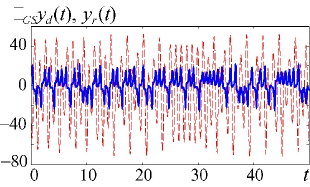
Figure 2: Time realization $y_{r}(t)$ corresponding to the autonomous dynamics of the Lorenz system (solid line) and $\varepsilon_{GS}y_{d}(t)$ (dashed line) corresponding to the external signal introduced into the response system near the onset of GS

In conclusion, we have explained GS appearance. The modified system approach has been proposed to demonstrate the reasons of GS arising. We have shown that the behavior of the response chaotic system is equal to the dynamics of the modified system (with the additional dissipation) under the external chaotic force. The coupling parameter increase is equivalent to the simultaneous growth of the dissipation and the amplitude of the external signal.

We thank Anastasiya E. Khramova, Olga I. Moskalenko and Alexander A. Tyschenko for the help in numerical experiments. We thank also Svetlana V. Eremina for English support. This work has been supported by U.S. Civilian Research & Development Foundation for the Independent States of the Former Soviet Union (CRDF, grant REC–006), Russian Foundation of Basic Research (project 05–02–16273), the Supporting program of leading Russian scientific schools (project NSch-1250.2003.2) and the Scientific Program “Universities of Russia” (project UR.01.01.371). We also thank “Dynastiya” Foundation.

References

- A. Pikovsky, M. Rosenblum, J. Kurths (2001) A. Pikovsky, M. Rosenblum, J. Kurths, Synchronization: a universal concept in nonlinear sciences (Cambridge University Press, 2001).
- K. Murali, M. Lakshmanan (1994) K. Murali, M. Lakshmanan, Phys. Rev. E 48, R1624 (1994).
- T. Yang, C.W. Wu and L.O. Chua (1997) T. Yang, C.W. Wu and L.O. Chua, IEEE Trans. Circuits and Syst. 44, 469 (1997).
- L. Glass (2001) L. Glass, Nature 410 (2001).
- P. Paoli, A. Politi, R. Badii (1989) P. Paoli, A. Politi, R. Badii, Physica D 36, 263 (1989).
- N.F. Rulkov, M.M. Sushchik, L.S. Tsimring, H.D.I. Abarbanel (1995) N.F. Rulkov, M.M. Sushchik, L.S. Tsimring, H.D.I. Abarbanel, Phys. Rev. E 51, 980 (1995).
- M.G. Rosenblum, A.S. Pikovsky, J. Kurths (1997) M.G. Rosenblum, A.S. Pikovsky, J. Kurths, Phys. Rev. Lett. 78, 4193 (1997).
- L.M. Pecora, T.L. Carroll (1990) L.M. Pecora, T.L. Carroll, Phys. Rev. Lett. 64, 821 (1990).
- R. Brown, L. Kocarev (2000) R. Brown, L. Kocarev, Chaos 10, 344 (2000).
- S. Boccaletti, J. Kurths, G. Osipov, D.L. Valladares, C.S. Zhou (2002) S. Boccaletti, J. Kurths, G. Osipov, D.L. Valladares, C.S. Zhou, Physics Reports 366, 1 (2002).
- S. Boccaletti, L.M. Pecora, A. Pelaez (2001) S. Boccaletti, L.M. Pecora, A. Pelaez, Phys. Rev. E 63, 066219 (2001).
- A.E. Hramov, A.A. Koronovskii (2004) A.E. Hramov, A.A. Koronovskii, Chaos 14, 603 (2004).
- K. Pyragas (1996) K. Pyragas, Phys. Rev. E 54, R4508 (1996).
- H.D.I. Abarbanel, N.F. Rulkov, M.M. Sushchik (1996) H.D.I. Abarbanel, N.F. Rulkov, M.M. Sushchik, Phys. Rev. E 53, 4528 (1996).
- L.M. Pecora, T.L. Carroll, J.F. Heagy (1995) L.M. Pecora, T.L. Carroll, J.F. Heagy, Phys. Rev. E 52, 3420 (1995).
- L.M. Pecora, T.L. Carroll (1991) L.M. Pecora, T.L. Carroll, Phys. Rev. A 44, 2374 (1991).
- K. Pyragas (1997) K. Pyragas, Phys. Rev. E 56, 5183 (1997).
- Z. Zheng, G. Hu (2000) Z. Zheng, G. Hu, Phys. Rev. E 62, 7882 (2000).