Energy localization in two chaotically coupled systems

Abstract

We set up and analyze a random matrix model to study energy localization and its time behavior in two chaotically coupled systems. This investigation is prompted by a recent experimental and theoretical study of Weaver and Lobkis on coupled elastomechanical systems. Our random matrix model properly describes the main features of the findings by Weaver and Lobkis. Due to its general character, our model is also applicable to similar systems in other areas of physics – for example, to chaotically coupled quantum dots.

1 Introduction

The statistical features of coupled systems have attracted considerable interest in many branches of physics. Random matrix theory (RMT) has been successfully used in many of those investigations. RMT was founded by Wigner [1]. It is a schematic model [2] in which the Hamiltonian, or, more generally, the wave operator of the system, is replaced by a random matrix. The necessary prerequisite is that the system be sufficiently “complex,” implying that the matrix elements of the Hamiltonian, or wave operator, calculated in an arbitrary basis, behave like random numbers. It has been shown that the spectral fluctuations in numerous different systems, if measured on the scale of the local mean-level spacing, are very well modeled by RMT; see the reviews in Refs. [3, 4, 5]. Due to the connection with chaos, one frequently refers to those systems as quantum chaotic which show correlations of RMT type. Similarly, systems are often referred to as regular if they lack spectral correlations.

We consider two coupled systems. We assume that either the two systems are chaotic before they are coupled or that the coupling itself introduces chaoticity if the separate systems are regular. This scenario is equivalent to the breaking of symmetries, if only two values of the quantum number belonging to that symmetry are taken into account. The statistical features crucially depend on the strength of the coupling measured on the scale of the local mean-level spacing. Many studies have been devoted to this issue of chaotically coupled systems or, equivalently, to symmetry breaking. We mention isospin breaking in nuclear physics [6, 7], symmetry breaking in molecular physics [8], symmetry breaking in resonating quartz crystals [9] and coupled microwave billiards [10]. While these studies addressed the spectral correlation, several investigations in nuclear physics [11, 12, 13, 14] focused on the statistics of the wave functions and related observables in the presence of symmetry breaking or similar effects. In all these cases, RMT approaches in the spirit of the Rosenzweig-Porter model [15] were successful.

Sometimes observables in the time domain such as spectral form factors are more appropriate than the eigenenergy correlations functions [2, 3, 4, 5]. This is so, for example, in the case of the presently much discussed fidelity; see Refs. [16, 17, 18, 19] and references therein. Another example is the study of the energy spread in chaotic systems [20, 21]. In the context of coupled systems, the time evolution of wave packets was investigated in Ref. [22].

In the present contribution, we study energy localization in two coupled systems in the time domain. This problem was addressed in a recent work by Weaver and Lobkis [23] who measured the time dependence of the wave intensity distribution in two coupled reverberation rooms. To this end, these authors recorded the time response to an elastic excitation of two coupled aluminum cubes. Moreover, they investigated the same problem theoretically and they numerically calculated the response in coupled two-dimensional membranes. In our study, we se tup and analyze an RMT model, based on the approaches in Refs. [15, 7, 13]. Its general character makes our model useful for similar problems in different physics contexts. In particular, we expect that our RMT approach also applies to coupled quantum dots.

The article is organized as follows. In Sec. 2 we sketch the work of Weaver and Lobkis [23]. In Sec. 3 we set up the RMT model and analyze it analytically and numerically. We compare our results to those of Weaver and Lobkis in Sec. 4. Discussion and conclusions are given in Sec. 5.

2 Experiment and numerical calculations

As we aim at a comparison with their findings, we present the work of Weaver and Lobkis [23] in some detail. Thereby, we also introduce the notation and conventions. The system studied experimentally consists of two aluminum cubes coupled by a solid connection, manufactured out of a solid aluminum block. The corners of the cubes were removed to desymmetrize the structure. This was done to ensure “chaotic” motion. Elastomechanical wave modes were excited in one room, and the response was measured in the other room. In this way, 16 different curves of energy intensity versus time were recorded, each in a small region around a different frequency. The results show that the energy does not always spread equally over the two rooms. If the coupling is weak, then the wave intensity is higher in the room where the initial excitation was performed than in the other room, regardless of how long one waits. Hence, the energy ratio never approaches unity. This deviation from the equipartition of the energy in the two rooms is referred to as energy localization. The resulting data are shown in Fig. 1, and as expected there is localization in the bins of larger mean-level spacing, but not in the bins of small mean-level spacing. We will discuss these results further in Sec. 4.

(a) Low frequency bins.

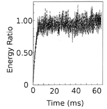
(b) High frequency bins.

Figure 1: Results from the experiment by Weaver and Lobkis. The energy ratio between the different rooms is plotted versus time (in ms). We note the different scales on the $y$ axes. Reprinted from Ref. [23].

Two numerical studies were performed on membranes with rough boundaries [23]. The dynamics of the system was in both cases governed by discretized wave equations in each of the rooms, and the coupling was realized in different ways in the two numerical calculations, to which we refer as N1 and N2 in the sequel. In the first one, N1, the connection had the form of a window between the two membranes similar to the situation in the experimental setup. In the second numerical calculation, N2, the rooms were separated, but springs were attached to a few different sites in rooms 1 and 2, thereby coupling those sites. In N1 and N2, a nonvanishing initial condition was given to one site in one of the rooms, and the response was calculated at different sites in the other room. The resulting time series were cosine-bell time windowed to focus on a specific instant in time. Then, the time series were Fourier transformed and integrated over a small region in frequency to accumulate data around a certain frequency. As in the experiment, 16 different curves of intensity versus time were obtained around different frequencies. At different frequencies, the systems have different effective couplings. Therefore, one expects [23] the time behavior of the different curves to differ in the degree of localization, as well as in the way in which this asymptotic saturation value is reached. Due to the differences in the coupling mechanism, there will also be differences between the results of N1 and N2.

Moreover, Weaver and Lobkis performed an analytical model study. The elastic wave equation for the state of the system $U(t)$, say, is of second order in time. To focus on the response in a narrow interval around a certain frequency $\Omega$, the ansatz $U(t)=u(t)\exp(-i\Omega t)$ is made with the assumption that $u(t)$ varies slowly with time. This leads to a first-order differential equation in time for $u(t)$ which has the form

$$-i\frac{\partial}{\partial t}u(t)=\frac{C+\Omega^{2}}{2\Omega}u(t)\ ,$$ (1)

where $C$ is the wave operator of the original second-order equation. The energies $E_{1}(t)$ and $E_{2}(t)$ in rooms 1 and 2 at time $t$ are defined as the total probability density of finding the system state $u(t)$ in one of the states $\psi_{ik},\ i=1,2$, which are good eigenstates in room $i$:

$$E_{i}(t)=\sum_{k}\left|u(t)\cdot\psi_{ik}\right|^{2}\ .$$ (2)

Strictly speaking, $E_{i}(t)$ is no energy. Nevertheless, we find this terminology introduced in Ref. [23] appropriate and use it as well, because $E_{i}(t)$ measures the degree of motion in room $i$. If no energy dissipates into the surrounding environment, the total energy $E=E_{1}(t)+E_{2}(t)$ is conserved – i.e., independent of time. In the sequel, it is always assumed that the system is excited in room 1, and the energy is measured in room 2. Analytical solutions for two coupled states are presented in Ref. [23] by employing different statistical assumptions.

3 Random matrix model

We set up the model in Sec. 3.1. The connection to the two-level form factor is established in Sec. 3.2, and a $2\times 2$ version of the model is evaluated in Sec. 3.3. We discuss numerical simulations of the RMT model in Sec. 3.4. Finally, we comment on chaotically coupled regular systems in Sec. 3.5.

3.1 Setup of the model

Spectral correlations in elastomechanics have been shown to be well described by RMT [24]. This is also true in the case of symmetry breaking [9], which is of direct relevance for the present study. Thus, RMT is also likely to be capable of modeling the time behavior of elastomechanical systems. As the first-order equation (1) has proved to be a good approximation to the experimental situation, we also base our model on this Schrödinger type of equation. Thus, it is more natural to replace $(C+\Omega^{2})/2\Omega$ by the random matrix $H$ than to replace $C$ itself. It turns out that this is indeed the best choice.

The appropriate RMT model is an extension of the one employed in Refs. [7, 13]. The random matrix $H$ modeling the operator $(C+\Omega^{2})/2\Omega$ reads

$$H=\left[\begin{array}[]{cc}H_{1}&0\\ 0&H_{2}\end{array}\right]+\alpha\left[\begin{array}[]{cc}0&V\\ V^{\dagger}&0\end{array}\right]\ .$$ (3)

The two matrices $H_{i},\ i=1,2$, model the uncoupled rooms 1 and 2. They are real symmetric and have random entries. We draw them from (two independent) Gaussian orthogonal ensembles (GOE’s). As the rooms in the experiments and the numerical calculations N1 and N2 were of the same size, the level densities were also the same. This can be adjusted in the RMT model by giving the matrices $H_{i}$ the same statistical weights and the same dimension $N$, such that $2N$ is the total dimension of $H$. The matrix $V$ also has random entries. The strength of the coupling is measured by the dimensionless parameter $\alpha$. It is sufficient to always assume $\alpha\geq 0$. The statistical weight of $V$ is chosen such that the total $H$ is in the GOE of $2N\times 2N$ matrices for $\alpha=1$.

We write the eigenvalue equation for the total Hamiltonian $H$ in the form

$$H\Psi_{n}=\omega_{n}\Psi_{n}\ ,\qquad n=1,\ldots,2N\ .$$ (4)

The eigenvalues $\omega_{n}$ and eigenvectors $\Psi_{n}$ are functions of the coupling parameter $\alpha$. It is convenient to introduce the notation

$$\Psi_{n}=\left[\begin{array}[]{c}\Psi_{1n}\\ \Psi_{2n}\end{array}\right]\ ,$$ (7)

where $\Psi_{in},\ i=1,2$, is the projection of $\Psi_{n}$ onto the subspace $i$. We emphasize that $\Psi_{in},\ i=1,2$, are functions of the coupling parameter $\alpha$. The eigenvalue equations for the Hamiltonians $H_{i}$ are written as

$$H_{1}\psi_{1n} = \omega_{1n}\psi_{1n}\ ,\qquad n=1,\ldots,N\ ,$$

$$H_{2}\psi_{2n} = \omega_{2n}\psi_{2n}\ ,\qquad n=1,\ldots,N\ ,$$ (8)

where the eigenvalues $\omega_{in}$ and eigenvectors $\psi_{in}$ are not functions of $\alpha$. This difference between $\Psi_{in}$ and $\psi_{in}$ is an immediate consequence of the fact that $H$ depends on $\alpha$, while $H_{1}$ and $H_{2}$ do not. We will also use the notation $\widehat{\psi}_{2n}=(0,\psi_{2n})^{\dagger}$ for the corresponding $2N$-dimensional vector with zeros in the first $N$ components.

At time $t=0$, the system is excited in room one such that the state of the total system can be written as

$$S=\left[\begin{array}[]{c}s\\ 0\end{array}\right]\ ,$$ (11)

where $s$ in room one is not specified in detail. We refer to $S$ as to the source. The time evolution of the source is then simply

$$u(t)=T(t)S\ ,\qquad{\rm where}\qquad T(t)=\exp\left(iHt\right)$$ (12)

is the time evolution operator. Using the eigenvectors $\widehat{\psi}_{2n}$, the energy in room 2 is thus given by

$$E_{2}(t,\alpha) = \sum_{n=1}^{N}\left|u(t)\cdot\widehat{\psi}_{2n}\right|^{2}=\sum_{n=1}^{N}\left(T(t)S\right)^{\dagger}\widehat{\psi}_{2n}\widehat{\psi}_{2n}^{\dagger}\left(T(t)S\right)$$ (15)

$$= S^{\dagger}T^{\dagger}(t)\left[\begin{array}[]{cc}0&0\\ 0&1_{N}\end{array}\right]T(t)S\ .$$

The block matrix only contains the unit matrix $1_{N}$ for room 2. We write $E_{2}(t,\alpha)$ instead of $E_{2}(t)$ to emphasize the dependence on the coupling parameter $\alpha$ in the RMT model. We will study averages $\overline{E_{2}}(t,\alpha)$ over the ensemble of matrices introduced in Eq. (3). Occasionally, we will also consider averages over the direction of the source. This average is denoted by angular brackets $\langle\cdots\rangle$.

The total energy $E$ is trivially conserved in the framework of our model. We have

$$E=E_{1}(t,\alpha)+E_{2}(t,\alpha)=S\cdot S=s\cdot s\ .$$ (16)

Hence, we can always construct $E_{1}(t,\alpha)$, once $E_{2}(t,\alpha)$ has been calculated.

As all correlations have to be measured [2, 3, 4, 5] on the local scale of the mean-level spacing $D$, we introduce an unfolded time $\tau=Dt$. This is also the scale on which $\alpha$ acts; we introduce the unfolded coupling parameter $\lambda=\alpha/D$. The energy on the unfolded scale is then given by

$$\varepsilon_{2}(\tau,\lambda)=\lim_{N\to\infty}\overline{E_{2}}(\tau/D,D\lambda).$$ (17)

Small values of $\alpha$ have a large effect on the correlation functions if the mean-level spacing $D$ is small as well.

3.2 Relation to the two-level form factor

We now derive an estimate for the time evolution of $E_{2}(t,\alpha)$ which should apply to strong coupling strength– i.e., to a parameter $\alpha$ which is large on the unfolded scale of the mean level spacing. If one assumes that the source $S$ comprises excitations into all states $\psi_{1n}$, one may average over the direction of the source. We find, from Eq. (15),

$$\langle E_{2}\rangle(t,\alpha)=B{\rm tr}^{(11)}\,T^{\dagger}(t)\left[\begin{array}[]{cc}0&0\\ 0&1_{N}\end{array}\right]T(t)\ ,$$ (20)

where ${\rm tr}^{(11)}$ is the trace over the $(11)$ sector of the whole matrix – i.e., over the upper left block. The constant $B$ results from the average. Expanding the time evolution operator in terms of the eigenvectors,

$$T(t)=\sum_{n=1}^{2N}\Psi_{n}\exp\left(i\omega_{n}t\right)\Psi_{n}^{\dagger}\ ,$$ (21)

we arrive after a short calculation at

$$\langle E_{2}\rangle(t,\alpha)=B\sum_{n,m}\left(\Psi_{1m}\cdot\Psi_{1n}\right)\left(\Psi_{2n}\cdot\Psi_{2m}\right)\exp\left[i(\omega_{n}-\omega_{m})t\right]\ .$$ (22)

The vectors $\Psi_{1n}$ and $\Psi_{2n}$ are, according to Eq. (7), the projections of the full eigenvector $\Psi_{n}$ onto the subspaces corresponding to the two rooms. They depend on the coupling parameter $\alpha$. These vectors coincide with the eigenvectors for the matrices $H_{1}$ and $H_{2}$ only for $\alpha=0$. Hence, they are only orthogonal in this special case. For all values $\alpha>0$, the scalar products $\Psi_{1m}\cdot\Psi_{1n}$ and $\Psi_{2n}\cdot\Psi_{2m}$ are neither zero nor given by $\delta_{nm}$. The ensemble average over the eigenenergies $\omega_{n}$ and over the eigenfunctions $\Psi_{n}$ decouples only for the parameter values $\alpha=0$ and $\alpha=1$– i.e., if the system either falls into two GOE’s or is represented by one GOE. We now estimate the ensemble average of the energy $\langle E_{2}\rangle(t,\alpha)$ by making the approximation that the averages over eigenenergies and eigenfunctions decouple. For strong coupling this should yield a reasonable result, and we will use this approximation in that limit only. We average over the eigenfunctions. For each term in the double sum in Eq. (22) the product of scalar products gives the same contribution which we can take out of the sums. Thus, we find

$$\overline{\langle E_{2}\rangle}(t,\alpha)=B\overline{\sum_{n,m}\exp\left[i(\omega_{n}-\omega_{m})t\right]}\ ,$$ (23)

where we absorbed the contributions from the average over the scalar products into the constant $B$. The average over the eigenvalues is yet to be performed. Luckily, the average in Eq. (23) is recognized as the Fourier transform of the two–level correlation function [2, 3]. This yields, on the unfolded scale,

$$\varepsilon_{2}(\tau,\lambda)=B\left[\delta(\tau/2\pi)+K_{2}(\tau/2\pi,\lambda)\right]\ ,$$ (24)

where the function $K_{2}(\tau,\lambda)$ is referred to as the two-level form factor. The term $\delta(\tau)$ is due to the diagonal contributions in the double sum of Eq. (23). We notice that the conventions used here require a rescaling of time with a factor of $2\pi$. The expression (24) is an estimate for the energy $\varepsilon_{2}(\tau,\lambda)$, exclusively in terms of the Fourier-transformed two-level spectral correlation function for the transition from two GOE’s to one GOE. Unfortunately, the two-level form factor is not known analytically for all values of $\lambda$. The result for one GOE, corresponding to $\lambda\to\infty$, reads [2]

$$K_{2}(\tau,\infty)=\left\{\begin{array}[]{ll}2\tau-\tau\ln(2\tau+1)&{\rm for}\quad 0<\tau\leq 1,\\ 2-\tau\ln\frac{{\textstyle 2\tau+1}}{{\textstyle 2\tau-1}}&{\rm for}\quad\tau\geq 1.\end{array}\right.$$ (25)

We notice that the function $\varepsilon_{2}(t,\infty)$ has the limit properties

$$\varepsilon_{2}(0,\infty) = 0,$$

$$\lim_{\tau\rightarrow\infty}\varepsilon_{2}(\tau,\infty) = B\ .$$ (26)

The second property will be used to fix the scale in comparison with the results of Ref. [23]. The estimate (24) should apply to large coupling – i.e., to parameter values $\lambda\gg 1$.

3.3 Two-by-two model

Quite often, one obtains surprisingly good information about an RMT model by restricting it to the smallest possible matrix dimension such that the nontrivial specific characteristics of the model are still present. This is successful in the case of the nearest-neighbor spacing distribution for the Gaussian orthogonal, unitary and symplectic ensembles (GGOE, GUE and GSE, respectively)  [3, 4, 5], but also for crossover transitions [25]. Here, we proceed analogously. We obtain a $2\times 2$ RMT model by setting $N=1$ in Eq. (3). It turns out convenient to absorb the parameter $\alpha$ into the matrix element $V$ such that

$$H=\left[\begin{array}[]{cc}H_{1}&V\\ V&H_{2}\end{array}\right]$$ (27)

and to readjust the probability density function $P(H)$ for the ensemble average accordingly:

$$P(H)=\frac{\sqrt{2}}{\pi\sqrt{\pi\alpha^{2}}}\exp\left(-H_{1}^{2}-H_{2}^{2}-2\frac{V^{2}}{\alpha^{2}}\right)\ .$$ (28)

As before, the GOE is recovered for $\alpha=1$. We introduce eigenvalue and angle coordinates

$$\left[\begin{array}[]{cc}H_{1}&V\\ V&H_{2}\end{array}\right]=\left[\begin{array}[]{cc}\cos\varphi&-\sin\varphi\\ \sin\varphi&\cos\varphi\end{array}\right]\left[\begin{array}[]{cc}\omega_{1}&0\\ 0&\omega_{2}\end{array}\right]\left[\begin{array}[]{cc}\cos\varphi&\sin\varphi\\ -\sin\varphi&\cos\varphi\end{array}\right]\ ,$$ (29)

which implies that the time evolution can be written in the same form with eigenvalues $\exp(i\omega_{1}t)$ and $\exp(i\omega_{2}t)$. For the integration measure one has

$$dH_{1}dH_{2}dV=\frac{1}{4}|\omega_{1}-\omega_{2}|d\omega_{1}d\omega_{2}d\varphi\ .$$ (30)

The source in this $2\times 2$ model is simply given by $S=(1,0)$. Thus, collecting everything, we find, with Eq. (15),

$$\overline{E_{2}}(t,\alpha) = \frac{\sqrt{2}}{4\pi\sqrt{\pi\alpha^{2}}}\int\limits_{-\infty}^{+\infty}d\omega_{1}\int\limits_{-\infty}^{+\infty}d\omega_{2}|\omega_{1}-\omega_{2}|\int\limits_{0}^{2\pi}d\varphi$$ (31)

$$\qquad\exp\left[-\frac{(\omega_{1}+\omega_{2})^{2}}{2}-\frac{(\omega_{1}-\omega_{2})^{2}}{2}\left(\cos^{2}2\varphi+\frac{\sin^{2}2\varphi}{\alpha^{2}}\right)\right]$$

$$\qquad\sin^{2}2\varphi\,\sin^{2}\frac{\omega_{1}-\omega_{2}}{2}t\ .$$

We introduce $x=(\omega_{1}+\omega_{2})/\sqrt{2}$ and $y=(\omega_{1}-\omega_{2})/\sqrt{2}$ as new integration variables, perform the $x$ and $\varphi$ integrals, and arrive at

$$\overline{E_{2}}(t,\alpha) = \frac{\alpha}{2(\alpha+1)}-$$ (32)

$$\qquad\alpha\int\limits_{0}^{\infty}dy\,y\,\exp\left[-y^{2}(1+\alpha^{2})\right]$$

$$\qquad\qquad\left[{\rm I}_{0}(y^{2}(1-\alpha^{2}))-{\rm I}_{1}(y^{2}(1-\alpha^{2}))\right]\cos 2\alpha yt\,.$$

Here, ${\rm I}_{0}$ and $\rm{I}_{1}$ denote the modified Bessel functions of zeroth and first order, respectively.

Formula (32) is the final result in the framework of our $2\times 2$ model. In Ref. [23], solutions for two-state models based on Eq. (1) with different statistical assumptions were given. Although the general behavior is similar to our $2\times 2$ RMT result (32), the analytical forms of these solutions in Ref. [23] are different.

For obvious reasons, the unfolding of formula (32) is meaningless. Nevertheless, experience with $2\times 2$ model for the spacing distribution tells that meaningful statements can be achieved if the transition parameter – i.e., the coupling strength $\alpha$ in our case – is interpreted properly. Here, we can do that in the following manner. For large times $t$, the function $\overline{E_{2}}(t,\alpha)$ becomes constant, because it reaches its saturation limit. The latter will depend on $\alpha$. Thus, comparing the saturation limit for the $2\times 2$ model with that of the $2N\times 2N$ RMT simulation or with those of the experiment and the numerical calculations N1 and N2 allows one, in principle, to interpret $\alpha$ on the unfolded scale. The saturation limit is easily obtained from Eq. (32). Due to the Riemann-Lebesgue lemma [26], we have

$$\lim_{t\to\infty}\overline{E_{2}}(t,\alpha)=\frac{\alpha}{2(\alpha+1)}\ ,$$ (33)

because the cosine function in the integrand oscillates so rapidly for large $t$, that the integral gives zero in the limit $t\rightarrow\infty$.

We notice that there is no equipartition of the energies for $t\to\infty$ at $\alpha=1$. This may seem a bit unexpected, because $H$ is a $2\times 2$ GOE matrix for that parameter value. It simply reflects the need to properly interpret the parameters, as just discussed. We study a two-state system and compare the probability for a transition between the two states with the probability of staying in one state. There is no reason why these should be equal. In the $N\rightarrow\infty$ limit, however, we expect equipartition for the full GOE. As the coupling parameter has to be measured on the scale of the local mean level spacing, the limit $N\rightarrow\infty$ corresponds to the limit $\alpha\rightarrow\infty$ in the $2\times 2$ version, and in that limit the right-hand side of Eq. (33) tends to $1/2$ and therefore to equipartition.

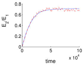
Figure 2: Energy ratio $E_{2}/E_{1}$ versus (dimensionless) time. Data from N1 of Ref. [23], bin 16, plotted as dashed line. The result from Eq. (24) for $\lambda\rightarrow\infty$, $B$ set by property 2 of Eq. (26) and a rescaling of time to make the two curves fit for early times, is plotted as a solid line.

(a) $2\times 2$ RMT model, fitted to N2 bins 2,3,4 from top to bottom.

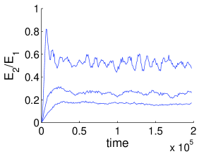
(b) Data from N2, bins 2,3,4 from top to bottom.

Figure 3: Comparison between the $2\times 2$ RMT model and the low frequency bins of N2 of Ref. [23]. The energy ratio $E_{2}/E_{1}$ is plotted versus (dimensionless) time.

3.4 Numerical simulations

The numerical simulations of the RMT model are performed as in Refs. [7, 13]. The unfolding of the results, however, is not done in the standard way. To compare with the numerical calculations of Weaver and Lobkis, it is more convenient to first unfold the level densities and then “refold” the spectra of our model with the level densities of Ref. [23]. Thereby we ensure that the mean-level densities of the RMT model acquire a form given by the Weyl formula for the billiardlike system of Ref. [23]. The appropriate Weyl formula for the modal density in a square membrane with Dirichlet boundary conditions reads [23]

$$\rho^{({\rm smooth})}(\Omega)=\frac{\Omega A}{2\pi c^{2}}-\frac{L}{4c}\ ,$$ (34)

depending on the frequency $\Omega$. Here, $A$ is the area of the membrane and $L$ is the side length of one room. Moreover, $c$ is the wave velocity and is chosen as unity here. Using twice the area of a room ($A=2\times 198^{2}$) and a value of $L$ which takes the roughness of the boundaries into account ($L=2\times 3\times 198$), we aquire an expression for the level density of the entire system. A comparison with the Weyl formula of Ref. [27] shows that the terms from the extra edges introduced to model the disorder cancel. Hence, we use the formula for a square membrane, which is precisely Eq. (34). This Weyl formula is employed to refold our RMT model for both numerical calculations N1 and N2. In the latter case, the system is not really a billiard, due to the springs used for the coupling. Nevertheless, the Weyl formula should be a good approximation to the real level density.

For every simulation, we generate random matrices of dimension $2N\times 2N=100\times 100$, unfold, refold, calculate $E_{2}(t,\alpha)$, and average over the results of 800 such simulations. As the functions $E_{2}(t,\alpha)$ are not measured on the unfolded scale, but on that of the Weyl formula, we do not introduce the notation $\varepsilon_{2}(\tau,\lambda)$ in the present context. Moreover, we notice that the numerical calculations N1 and N2 depend on the mean frequency $\Omega$ in the bin under consideration. Accordingly, we arrive at a two-parameter family of time-dependent curves $\overline{E_{2}}(t,\alpha,\Omega)$. We now associate each bin in the numerical calculation performed by Weaver and Lobkis with the corresponding frequency $\Omega$. This leaves us with a one-parameter family of time-dependent curves $\overline{E_{2\mu}}(t,\alpha),\ \mu=1,\ldots,16$, for each bin labeled by $\mu$.

3.5 Chaotically coupled regular systems

In the RMT model defined by Eq. (3) and in its subsequent analysis, we always drew the matrices $H_{i},\ i=1,2$, from (two independent) GOE’s, implying that we model the two rooms individually as chaotic systems — before the coupling is considered. One can also assume that the two rooms are regular systems before they are coupled. In that case, the matrices $H_{i},\ i=1,2$, would be drawn from Poisson ensembles [3]. We also did such numerical simulations. The results are qualitatively the same if the coupling – i.e., the matrix $V$ – introduces enough chaos. The main effect is an adjustment of the scales. What matters for the qualitative behavior is the chaoticity of the total system.

4 Comparison with experiment and numerical calculations

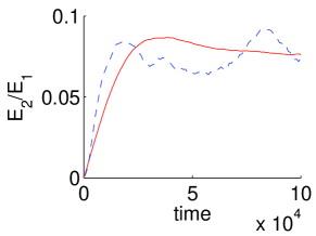
(a) Bin 2.

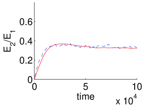
(b) Bin 5.

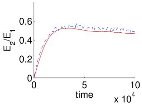
(c) Bin 9.

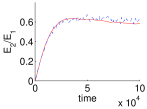
(d) Bin 13.

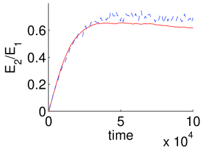
(e) Bin 16.

Figure 4: Energy ratio $E_{2}/E_{1}$ versus (dimensionless) time. Data from N1 of Ref. [23] plotted as dashed lines and from refolded numerical simulations using the RMT model as solid lines. We notice the different $E_{2}/E_{1}$ scale in plot (a).

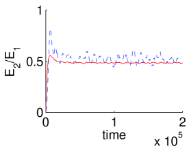
(a) Bin 2.

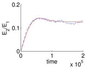
(b) Bin 5.

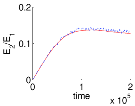
(c) Bin 9.

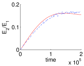
(d) Bin 13.

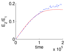
(e) Bin 16.

Figure 5: Energy ratio $E_{2}/E_{1}$ versus (dimensionless) time. Data from N2 of Ref. [23] plotted as dashed lines and from refolded numerical simulations using the RMT model as solid lines. We notice the different $E_{2}/E_{1}$ scale in plot (a).

We now compare the results of our RMT model with those of Ref. [23]. The quantity studied in Ref. [23] is mostly the fraction of energy in room 2, or $E_{2}(t)/E$. In our figures, we plot $E_{2}(t)/E_{1}(t)$ instead. We first consider the estimate, Eq. (25), involving the GOE form factor and the result (24) of the $2\times 2$ RMT model and compare with the numerical calculations N1 and N2. As formula (24) was derived under the assumption of strong coupling on the scale of the local mean-level spacing, it should apply to the high-frequency bins of N1. Anticipating the later extraction of the coupling parameter, we already now mention that indeed $\lambda>1$ in that bin. In Fig. 2 we compare Eq. (24) with data from bin 16 (the highest frequency bin) of N1. A good description is obtained, although no equipartition is reached. This implies that the effective coupling $\lambda$ is large, but not very large. We recall that formally $\lambda\to\infty$ corresponds to the strongest coupling $\alpha=1$ – i.e., to one single system. Expansion of the form factor for short times $\tau$ reveals a linear short time dependence of the ensemble-averaged energy $\varepsilon_{2}(\tau,\lambda)$. This is in agreement with the analytical discussion of Ref. [23].

Table 1: Coupling parameters $\alpha$ for the $2\times 2$ model used in Fig. 3(a). The asymptotic saturation $E_{2}/E$ values for N2 in bins 2, 3, and 4 are taken from Ref. [23]. The corresponding coupling parameters are calculated from Eq. (33).

bin	$E_{2}/E$ (asymptotic)	$\alpha$
2	0.35	2.33
3	0.2	0.67
4	0.14	0.39

We turn to the $2\times 2$ RMT model and compare to bins 2, 3, and 4 of N2. The values of the coupling parameter $\alpha$ are determined from Eq. (33) and given in Table  1, together with the $E_{2}/E$ saturation values of N2. The $2\times 2$ RMT model curves and data from N2 are shown in Figs. 3(a) and 3(b), respectively. As expected, smaller values of $\alpha$ correspond to a higher degree of localization – i.e., to a stronger deviation from equipartition. The general behavior of the results from the $2\times 2$ model stays the same for large values of $\alpha$. We notice that the time scale is different, because the data from N2 were not unfolded. The similarity shown in Fig. 3 between the $2\times 2$ RMT model and the Weaver-Lobkis results [23] is remarkable. This parallels the success of $2\times 2$ RMT models for the spacing distributions.

The RMT simulations yield a one-parameter family of curves for each bin, to be compared with the numerical calculations N1 and N2. We use visual inspection to determine, for each bin, which curve fits best to the numerical calculations N1 and N2. Typical results for some of the bins are shown in Figs. 4 and 5. In the low-frequency bins of N2 there is a discrepancy; see Fig. 5(a). The RMT simulation does not overshoot its saturation value as clearly as the data of Ref. [23]. This very large overshoot within a short-time interval is, however, borne out in the $2\times 2$ RMT model; see Fig. 3. By the visual fit we determine the coupling parameter $\alpha$. We measure it on the scale of the local mean-level spacing. In Table  2, we list the in this manner obtained coupling parameter $\lambda$ for N1 and N2 for the bins under consideration. The $\lambda$ values extracted for N1 go up with higher bins, because the saturation value comes closer to equipartition. This effect is also visible for N2, but not so pronounced, because the saturation value does not change much for higher bins.

Table 2: Coupling constants $\lambda$ on the unfolded scale resulting from the RMT simulation, determined for some bins of the numerical calculations N1 and N2 with mean frequencies $\Omega$: see Figs. (4) and (5).

bin	$\Omega$	$\lambda$ for N1	$\lambda$ for N2
2	0.1562	0.4750	3.2316
5	0.4686	2.0222	0.7754
9	0.8851	3.0586	0.7502
13	1.3016	3.9093	0.8441
16	1.6140	4.2427	0.8899

We find good qualitative agreement between the RMT simulation and N1 and N2. Importantly, fluctuations between different random matrices are quite large, and the RMT curves presented here are averages of $E_{2}$ over 800 random matrices. Among those some show very much closer similarity to the curves of Weaver and Lobkis [23], and we believe that most of the discrepancy in the low-frequency bins of N1 are due to fluctuations resulting from the specific choice of the boundary and perhaps other parameters in the numerical calculations of Ref. [23]. The reason for this interpretation of the discrepancy is the peculiar form of the fluctuations in bin 2 of N1; see Fig. 4(a). Since these lower bins have a lower level density, they should also be more sensitive to this kind of fluctuations. In the intermediate-frequency bins, we find that the numerical calculations N1 and N2 are well reproduced by the RMT model. In the figures for the high-frequency bin, Figs. 4(e) and 5(e), the RMT results are seen to deviate downwards for large times. It is conceivable that the short-time behavior strongly depends on the specific realization of the coupling while the long-time behavior is universal.

The result from the experiment is shown in Fig. 1. The qualitative features are well described by the RMT model. It can be seen that the system localizes in the low-frequency bins, but does not do so in the high-frequency bins. In other words, the system approaches equipartition of the energy. The localization behavior depends on the strength of the coupling measured on the scale of the local mean-level spacing, and the mean-level density is significantly higher in the high-frequency bins. It seems that the saturation value has not yet been reached on the time scale visible in Fig. 1. A closer inspection shows an initial behavior similar to the one in the results from our numerical RMT calculations and a slight upwards trend of the energy ratio towards the end of the time window studied. According to Ref. [23] this means that, first, the expected asymptotic value of $E_{2}/E_{1}$ is reached in the middle of the time window studied and that, second, there is another unknown effect acting on longer time scales adding to the energy spread which is likely to be due to the coupling of the setup to the environment. Thus, we do not attempt to extract a quantitative estimate of the coupling parameter $\alpha$ for the experiment.

5 Conclusion

We have set up and analyzed an RMT model to describe the time behavior of coupled reverberation rooms. This system shows localization effects under certain conditions. Within our RMT model, we gave an estimate of the strong coupling behavior which involved the two-level GOE form factor. Moreover, we studied the $2\times 2$ version of our RMT model analytically for arbitrary coupling strength and performed numerical simulations for the $2N\times 2N$ version.

From the comparison with the work of Weaver and Lobkis, we conclude that the RMT model yields a good qualitative description. Moreover, we find an interpretation of the localization effect by relating it to the universal features of RMT models for crossover transitions.

Formally similar RMT models have been studied in connection with symmetry breaking. Then, the parameter $\alpha$ measures the degree of symmetry breaking. This is so for isospin breaking in nuclear physics [6, 7, 11, 13], symmetry breaking in molecular physics [8], and symmetry breaking in resonating quartz crystals [9]. The experiment that comes closest to the present situation is the study of spectral correlations in coupled microwave billiards [10]. In this work and in the experiment of Weaver and Lobkis [23], an excitation initially in system one would stay there for all times if the coupling is zero. This is formally analogous to a conserved quantum number.

In the RMT model the parameter measuring the size of the connection has a most natural counterpart: the root-mean-square matrix element due to the coupling measured on the scale of the local mean-level spacing. Thus, there are two ways of making the effective, dimensionless coupling parameter $\lambda$ small and to thereby introduce localization: either the original coupling parameter $\alpha$ which always has a dimension is small or the mean-level spacing $D$ is made large.

It might be surprising that no equipartition of the energy is seen for all coupling strengths even if one waits very long. This would be the expectation if one compares the system with two water basins coupled by a channel. Suppose that initially the two basins are empty and the channel is closed by a gate. Now one of the basins is filled with water and the gate is opened at $t=0$. Obviously, the water levels in the two basins will be equal after sufficiently long time. The speed with which this equipartition is reached simply depends on the cross section of the channel.

In the present case of the two coupled acoustic rooms the situation is different, because the wave character of the excitations has to be taken into account. Thus, the crucial parameter entering is the size of the coupling connection – i.e., its geometrical width – compared to a typical wavelength. The first waves after the excitation which come from system 1 into system 2 enter a silent territory and cause the first excitations there. The next waves coming from system 1, however, encounter these first excitations in system 2 and interfere with them constructively or destructively. This process continues and, of course, after being excited in system 2, waves also travel back into system 1. For smaller times, this complicated dynamics certainly depends strongly on the realization of the coupling. This is clearly so in the numerical calculation of Ref. [23]. Nevertheless, the loneg-time behavior, in particular the saturation limit, shows universal characteristics, consistent with general features of quantum chaotic systems; see Ref. [3]. In the energy domain, this is borne out in the fact that the correlations on smaller energy scales are described by universal RMT features, while system-specific properties show up on larger scales, leading to deviations from the RMT prediction. To avoid confusion, we emphasize that these universal RMT features include those in the presence of symmetry breaking. By system-specific properties we mean, most importantly, the scales set by the shortest periodic orbits.

It is worthwhile to realize that the chaoticity of the individual subsystems before the coupling is not crucial, if the coupling itself introduces enough chaos. We tested numerically that the behavior of the corresponding model for two regular subsystems coupled chaotically shows the same qualitative behavior. The saturation value is reached slightly faster, which simply means that time is rescaled. Finally, we mention that our model is not restricted to elastomechanics. It would also apply to coupled quantum dots and other coupled systems.

References

- [1] E.P. Wigner, reprinted in Statistical Theories of Spectra: Fluctuations, edited by C.E. Porter (Academic Press, New York, 1965), p. 199.
- [2] M. L. Mehta, Random Matrices, 2nd ed. (Academic Press, New York, 1991).
- [3] T. Guhr, A. Müller -Groeling, and H.A. Weidenmüller, Phys. Rep. 299, 189 (1998).
- [4] H.J. Stöckmann, Quantum Chaos –An Introduction (Cambridge University Press, Cambridge, England, 1999).
- [5] F. Haake, Quantum Signatures of Chaos, 2nd ed. (Springer-Verlag, Berlin, 2001).
- [6] G.E. Mitchell, E.G. Bilpuch, P.M. Endt, and J.F. Shriner, Jr., Phys. Rev. Lett. 61, 1473 (1988).
- [7] T. Guhr and H.A. Weidenmüller, Ann. Phys. (N.Y.) 199, 412 (1990).
- [8] D.M. Leitner, Phys. Rev. E 48, 2536 (1993); D.M. Leitner, H. Köppel, and L.S. Cederbaum, Phys. Rev. Lett. 73, 2970 (1994).
- [9] C. Ellegaard, T. Guhr, K. Lindemann, J. Nygård, and M. Oxborrow, Phys. Rev. Lett. 77, 4918 (1996).
- [10] H. Alt, C.I. Barbosa, H.D. Gräf, T. Guhr, H.L. Harney, R. Hofferbert, H. Rehfeld, and A. Richter, Phys. Rev. Lett. 81, 4847 (1998).
- [11] A.A. Adams, G.E. Mitchell, and J. F. Shriner, Jr., Phys. Lett. B 422, 13 (1998).
- [12] A.A. Adams, G. E. Mitchell, W.E. Ormand, and J. F. Shriner, Jr., Phys. Lett. B 392, 1 (1997).
- [13] C.I. Barbosa, T. Guhr, and H.L. Harney, Phys. Rev. E. 62, 1936 (2000).
- [14] A. Hamoudi, R.G. Nazmitdinov, E. Shahaliev, and Y. Alhassid, Phys. Rev. C. 65, 064311 (2002).
- [15] N. Rosenzweig and C.E. Porter, Phys. Rev. 120, 1698 (1960).
- [16] N.R. Cerruti and S. Tomsovic, J. Phys. A. 36, 3451 (2003).
- [17] G. Benenti, G. Casati, and G. Veble, Phys. Rev. E. 68, 036212 (2003).
- [18] T. Prosen, T.H. Seligman, and M. Znidaric, Prog. Theor. Phys. Suppl. 150, 200 (2003).
- [19] J. Vanicek, and E.J. Heller Phys. Rev. E. 68, 056208 (2003).
- [20] D. Cohen, F.M. Izrailev, and T. Kottos, Phys. Rev. Lett. 84, 2052 (2000).
- [21] T. Kottos and D. Cohen, Phys. Rev. E. 64, 065202 (R) (2001).
- [22] O. Bohigas, S. Tomsovic, and D. Ullmo, Phys. Rep. 223, 43 (1993).
- [23] R.L. Weaver and O. Lobkis, J. Sound Vib. 231, 1111 (2000).
- [24] R.L. Weaver, J. Acoust. Soc. Am. 85, 1005 (1989).
- [25] G. Lenz and F. Haake, Phys. Rev. Lett 65, 2325 (1990).
- [26] I.S. Gradshteyn and I.M. Ryzhik, Table of Integrals, Series and Products, (Academic Press, New York, 2000).
- [27] M.V. Berry, Ann.Phys. (N.Y.) 131, 163 (1981).