Dynamics of fluctuation of the top location of a sandpile

Abstract

We investigate the fluctuation of the top location of a sandpile numerically using the two-dimensional discrete elements method. We feed particles to a sandpile at a fixed time interval and calculate power spectra from the time series of the top location. We find that the power spectra are approximated as power functions, and their exponents increase to $-1$ through a plateau as the time interval decreases. For small time interval, avalanches occur continuously either on the left or right side slope of a sandpile, and the slope on which avalanches take place switches intermittently. The long time fluctuation of the top location corresponds to the switchings. For the time series of the switchings, we discuss the relation between the power spectrum and the distribution of waiting times based on analytic theories.

1 Introduction

Dense systems of granular materials exhibit solid-like and fluid-like behaviors [1, 2, 4, 3], and many researches are devoted on them. For the static phase, the spatial distribution of stress on the bottom of a sandpile was measured in experiments, and it is known that its functional form depends on the history of the formation of the sandpile [5, 6, 7, 8]. For the fluid phase, steady flows and avalanches are investigated from several perspectives [9, 10, 11, 12, 13, 14, 15, 16, 17, 18]. Fluidized phase appears in a localized layer near the surface, and the particle velocity under the layer obeys an exponential function of the depth from the surface [19]. It is known for granular flows in a pipe that the temporal power spectra of particle density obey power laws [20, 21, 22, 23, 24, 25, 26, 30, 27, 28, 29, 31].

In systems of a sandpile, feeding particles at small feed rate, the surface of a sandpile is kept in solid states except when avalanches occur intermittently, and continuous flows appear as the feed rate increases. However, even in the case that the feed rate is rather large, it is infrequent that the whole surface of a sandpile is kept in the fluid phase, and the states of the surface change temporally or spatially [32]. The time evolution of a sandpile is caused by complicated interactions between avalanches and the shape of the surface.

A sandpile typically becomes mountain shaped with a top as it grows [33, 34]. Because particles on the surface run down from the top to the foot of a sandpile, the top plays the role of a singular point in an average flow of particles. In the formation process of a sandpile, the top location moves with time and determines the global flow on the surface. In this paper, we focus on the fluctuation of the top location to characterize the long time evolution of a sandpile. We carry out two-dimensional numerical simulations and measure the power spectrum of the top location. We find that the power spectrum obeys a power function, and that the exponent depends on the feeding rate.

The organization of the remainder of this paper is as follows. In §2, we explain the method of our numerical simulations. In §3, we investigate the power spectrum of the top location and relations between its exponent and the feed rate of particles. In §4, we discuss the origin of this power law. Finally, we draw conclusions in §5.

2 Method Of Simulations

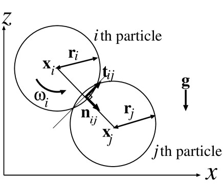
Figure 1: The $i$th particle and the $j$th particle are in contact.

In order to simulate polydispersed circular particles, we adopt a two-dimensional Discrete Elements Method (DEM) [35]. In DEM, we assume that particles are cohesionless, and the mass density of a particle per unit area, $\rho_{0}$, is constant. The linear spring model is adopted to describe the repulsion of two particles in contact, and the viscous forces and Coulomb slip are assumed to act on them. We assume that the $i$th particle has the radius $r_{i}$, the mass $m_{i}=\pi r_{i}^{2}\rho_{0}$ and the momentum of inertia $I_{i}=m_{i}r_{i}^{2}/2$. The center of mass and the angular velocity of the $i$th particle represent $\mathbf{x}_{i}$ and $\omega_{i}$, respectively. The equations of motion of the $i$th particle are given by

$$\begin{array}[]{rcl}m_{i}\ddot{\mathbf{x}}_{i}&=&\sum_{j}\Bigl{(}F_{n}^{ij}\mathbf{n}_{ij}+F_{t}^{ij}\mathbf{t}_{ij}\Bigr{)}+m_{i}\mathbf{g},\\ I_{i}\dot{\omega}_{i}&=&r_{i}\sum_{j}F_{t}^{ij},\end{array}$$ (3)

where $\mathbf{n}_{ij}$ and $\mathbf{t}_{ij}$ represent the normal and the tangential unit vectors at the contact point between the $j$th particle and the $i$th particle, and $\mathbf{g}$ is the acceleration of gravity, as depicted in Fig. 1. The normal contact force $F_{n}^{ij}$ is defined by

$$F_{n}^{ij}=\tilde{F}_{n}^{ij}\Theta(-\tilde{F}_{n}^{ij}),$$ (4)

and

$$\tilde{F}_{n}^{ij}=-k_{n}m_{r}^{ij}\Bigl{(}r_{i}+r_{j}-|\mathbf{x}_{i}-\mathbf{x}_{j}|\Bigr{)}-\eta m_{r}^{ij}\mathbf{n}_{ij}\cdot\Bigl{(}\dot{\mathbf{x}}_{i}-\dot{\mathbf{x}}_{j}\Bigr{)},$$ (5)

where $\Theta(x)$ is the Heaviside function, and $m_{r}^{ij}$ is the reduced mass $m_{r}^{ij}\equiv\frac{m_{i}m_{j}}{m_{i}+m_{j}}$. $\Theta(-x)$ is introduced so that the contact force is repulsive. The tangential contact force $F_{t}^{ij}$ is defined by

$$F_{t}^{ij}=k_{t}m_{r}^{ij}u_{t}^{ij}.$$ (6)

$u_{t}^{ij}$ is obtained by integrating the equation

$$\dot{u}_{t}^{ij}=-\Bigl{(}(\dot{\mathbf{x}}_{i}-\dot{\mathbf{x}}_{j})\cdot\mathbf{t}_{ij}+r_{i}\omega_{i}+r_{j}\omega_{j}\Bigr{)}\Theta\bigl{(}\mu|F_{n}^{ij}|-|F_{t}^{ij}|\bigr{)},$$ (7)

where $u_{t}^{ij}$ is zero when the particles are not in contact (i. e. for $|\mathbf{x}_{j}-\mathbf{x}_{i}|>r_{j}+r_{i}$). Here, Coulomb frictional coefficient $\mu$ is assumed to be $0.5$. We express the maximum diameter and the maximum weight of a particle as $d$ and $m$. The distribution function of the diameters is uniform in the range between $0.8d$ and $d$. We assume that the spring constants are $k_{n}=1.0\times 10^{4}mg/d$ in the normal direction, and $k_{t}=2.0\times 10^{3}mg/d$ in the tangential direction, and that the viscosity is $\eta=1.0\times 10^{2}\sqrt{g/d}$. The coefficient of restitution in our model is about $0.2$ for a head-on particles collision. We adopt the second-order Adams-Bashforth method for time-integration with the time interval $\Delta t=1.0\times 10^{-3}\sqrt{d/g}$.

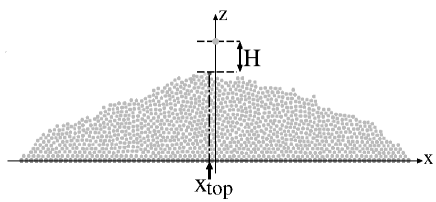
Figure 2: Setup of a sandpile in our simulations. $x_{top}$ represents the horizontal top location. Fed particles are released at the height $H$ from the top.

We assume that a particle is in a sandpile if the particle contacts other particles, and the top location of the sandpile is defined as the center of mass of the highest particle in the sandpile (Fig. 2). The floor under a sandpile is a horizontal array of $80$ fixed particles with diameter $d$. We introduce the $x$ coordinate along the floor and define the origin at the center of the floor.

To investigate the fluctuation of the top in the formation process of a sandpile, we drop particles with the time interval $T$ to it. The particles are released at a position just above the center of the floor and its height is $H$ from the top location as shown in Fig. 2. We first make a sandpile grow until it covers the floor and use this sandpile as an initial state. Because particles run off the edges of the floor with finite length, the size of a sandpile is maintained almost constant.

After the time series of the top location $x_{top}(t)$ reaches a statistical stationary state, we calculate its power spectrum $S(f)$ with respect to frequency $f$. To calculate the power spectrum $S(f)$ from the time series, we divide it into $M$ time series with a time interval $T^{(s)}$, the $m$th power spectrum $S_{m}(f_{j})$ is defined by

$$S_{m}(f_{j})\equiv\frac{1}{N}|\sum_{n=1}^{N}x_{top,n}^{(m)}e^{-\frac{2\pi in}{N}j}|^{2}$$ (8)

where $x_{top,n}^{(m)}\equiv x_{top}((m+\frac{n}{N})T^{(s)})$ and $f_{j}\equiv\frac{j}{T^{(s)}}$.

We introduce the power spectrum $S(f)$ as the average of the $M$ power spectra,

$$S(f_{j})\equiv\frac{1}{M}\sum_{m=0}^{M-1}S_{m}(f_{j}).$$ (9)

3 Results

Figure 3: Time series of the top location $x_{top}(t)$. We use $H=110d$, $T=2\sqrt{d/g}$ (a) and $T=80\sqrt{d/g}$ (b). The vertical axes are time $t$. We note that the same number of particles are fed in (a) and (b).

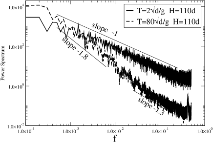
Figure 4: Double logarithmic plot of $S(f)$ for the time series. $H=110d$, $T=2\sqrt{d/g}$ (black line) and $T=80\sqrt{d/g}$ (dashed line). The lines are drawn for reference.

We measure $x_{top}$ for various values of the time interval $T$ and the height $H$. We change $H$ in the range $20d\leq H\leq 110d$. If $H$ is sufficiently large beyond this range, the impact of a dropped particle is large and collapses the top shape of a sandpile into a caldera [36]. Figures 3(a) and 3(b) shows the time series of $x_{top}(t)$ obtained from simulations with $T=2\sqrt{d/g}$ (a) and $T=80\sqrt{d/g}$ (b). The top fluctuates frequently in the case of small $T$, on the other hand, in the case of large $T$, the top almost stays for long time in comparison with $T$ because the motion of particles induced by the impact of a fed particle ceases before the next particle is dropped. Figure 4 is the power spectra of the time series, $S(f)$, which is calculated using eqs. (8) and (9) with $T^{(s)}=N=10000$ and $M=10$. We find that $S(f)$ behaves as a power-law, and its exponent depends on the value of $T$. At $T=2\sqrt{d/g}$, $S(f)$ approximately obeys $1/f$ law. At $T=80\sqrt{d/g}$, the exponents of $S(f)$ are smaller than $-1$.

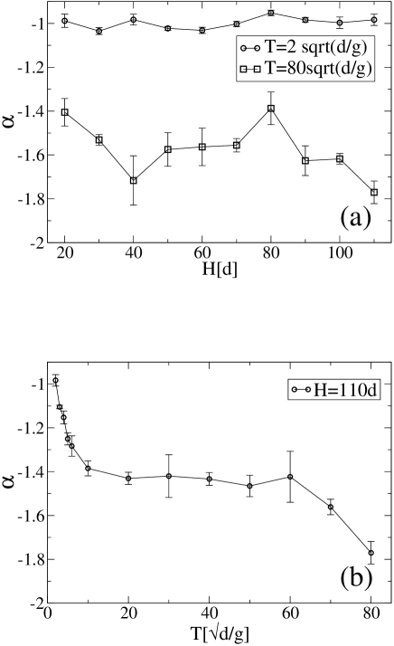
Figure 5: (a) Dependence of $\alpha$ on $H$ and (b) dependence of $\alpha$ on $T$. The error bars correspond to the standard deviations.

We investigate the dependence of the exponent of $S(f)$, $\alpha$, on $T$ and $H$. For the range $5/T^{(s)}\leq f\leq 1/(2T)$, we calculate $\alpha$ from the double logarithmic plot of $S(f)$ in the least square method. $\alpha$ is insensitive to $H$ as shown in Fig. 5(a). In contrast, Fig. 5(b) indicates that $\alpha$ strongly depends on $T$ for small $T$ and approaches $-1$ as $T$ decreases. As $\alpha$ approaches $-1$, the power spectrum is approximated as a power function with a high degree of accuracy as indicated with the error bars. In the range $10\sqrt{d/g}<T<60\sqrt{d/g}$, $\alpha$ is approximately a constant $-1.43\pm 0.03$, although $\alpha$ decreases as $T$ increases beyond $60\sqrt{d/g}$. In the case of large $T$, the error bars in Figs. 5 are large because the range of frequency used for fitting is small. In the region of higher frequency than $1/T$, the power function with the same exponent is not best fit with $S(f)$. If we fit $S(f)$ with a power function in this range of high frequency, its exponent changes from that indicated in Figs. 5, as shown with the data of $T=80\sqrt{d/g}$ in Fig. 4.

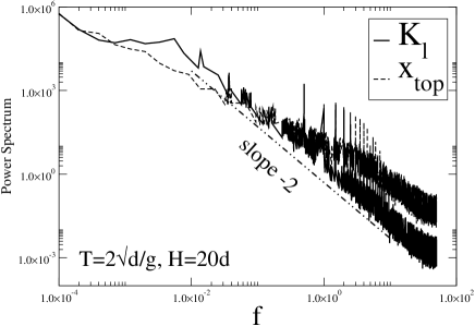
Figure 6: Power spectra of the time series of $x_{top}(t)$ and $K_{l}(t)$ for $T=2\sqrt{d/g}$ and $H=20d$. The line with a slope is drawn for reference.

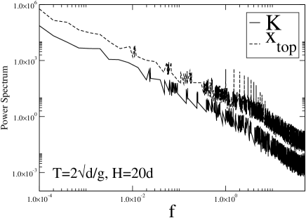
Figure 7: Power spectra of the time series of $x_{top}(t)$ and $K(t)$ for $T=2\sqrt{d/g}$ and $H=20d$.

We mainly focus on the case of small $T$ because we are, in particular, interested in the case that $\alpha$ is close to $-1$. The displacement of the top location $x_{top}$ is caused by avalanches, and avalanches occur on either slope at almost all times in this case. Although the instantaneous magnitude of avalanches is characterized by the kinetic energy of the particles, $S(f)$ and the power spectrum of the kinetic energy differ in functional form as mentioned below. Eliminating the narrow region $-d\leq x\leq d$ in the center of a sandpile, we divide the sandpile into the left part and the right part with respect to $x=0$. We measure the kinetic energies of the left and right parts, $K_{l}(t)$ and $K_{r}(t)$, respectively. Using the same definition in eqs. (8) and (9), the power spectra of the time series of $K_{l}(t)$ and $K_{r}(t)$ are calculated with $T^{(s)}=1.0\times 10^{4}\sqrt{d/g}$, $N=1.0\times 10^{5}$ and $M=10$. For $T=2\sqrt{d/g}$ and $H=20d$, the power spectra of both $K_{l}(t)$ and $x_{top}(t)$ are shown in Fig. 6. The power spectrum of $K_{r}(t)$ is similar to that of $K_{l}(t)$. Because the power spectra of $K_{l}(t)$ and $K_{r}(t)$ are Lorentzian-like, avalanches seem to occur at random.

From the results of numerical simulations, it is found to be rare that avalanches occur simultaneously on the left and right slopes of a sandpile. We refer the states that avalanches occur on the left and right slopes as left mode and right mode, respectively. To investigate switchings between the both mode, we define the binarized time series,

$$K(t)=\begin{cases}+1,&\text{for $K_{l}(t)<K_{r}(t)$},\\ -1,&\text{for $K_{l}(t)\geq K_{r}(t)$}.\end{cases}$$ (10)

The sign of $K(t)$ represents the side on which avalanches occur mainly at time $t$. The switchings are well defined by $K(t)$ in the case that $T$ is small. However, as $T$ increases, it is difficult to define the switchings because avalanches occur at intervals, and the time intervals between avalanches are comparable to the time scale of switchings. We find that the time series of $K(t)$ is similar to $x_{top}(t)$ for small $T$. The power spectrum of the time series $K(t)$ is shown in Fig. 7 for $T=2\sqrt{d/g}$ and $H=20d$. The power spectrum of $K(t)$ is approximated as a power law with the exponent of $-1$ in the long time scale. The exponent is approximately the same as that of the top location. Investigating the conditional probability of $K(t)=-1$ for a given $x_{top}$, this probability increases with the value of $x_{top}$. Therefore, in each mode, the top location $x_{top}(t)$ is mainly in the opposite side on which avalanches occur. Thus the fluctuation of $x_{top}$ corresponds to the switching between the two modes, but not to the fluctuation of the magnitude of avalanches.

4 Discussion

For the binarized time series such as $K(t)$ defined by eq. (10), it is known from an analytical theory that its spectrum is expressed as a power function if the waiting time has a power-law distribution and each interval is independent [37, 38]. Here, the waiting time $\tau$ is defined as a time interval between neighboring switchings in the binarized time series. We assume that the probability density of $\tau$, $p(\tau)$, is the abrupt-cutoff power law,

$$p(\tau)=\begin{cases}ct^{D},&\text{for $a<t<b$},\\ 0,&\text{otherwise},\end{cases}$$ (11)

where the constants $a$ and $b$ are sufficiently small and large respectively, and $c$ is the normalization constant. In the range of $1/b\ll f\ll 1/a$, the power spectrum of this binarized time series, $S_{b}(f)$, is given approximately by

$$S_{b}(f)\sim f^{-(D+3)}$$ (12)

for $-3<D<-1$. In the case of small $T$, $p(\tau)$ is expected to be a power function with $D\cong-2$ because the exponent of the power spectrum of $K(t)$ is approximately $-1$ in our simulations. However there are few intervals with waiting time longer than $\tau\cong 100\sqrt{d/g}$ in $K(t)$ because small noises chop up long intervals. Therefore applying the median filter of a time width of $60\sqrt{d/g}$ to $K(t)$, we calculate the distribution of waiting time for the coarse-grained time series, $p(\tau^{{}^{\prime}})$. We find that $p(\tau^{{}^{\prime}})$ decays approximately as a power function with $D\cong-2$ as shown in Fig. 8.

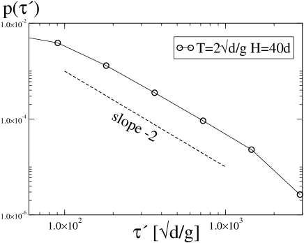
Figure 8: The distribution of the waiting time in $K(t)$ for $T=2\sqrt{d/g}$ and $H=40d$.

The plateau with $\alpha\cong-1.4$ appears in a wide range of $T$ as shown in Fig. 5(a), although the switchings can not be well-defined by $K(t)$ as $T$ increases. It is possible that the dynamics of the top location has some relations with the density fluctuation of flows. In experiments of granular flow in vertical pipes filled with fluid, the exponents $-1$, $-4/3$ and $-3/2$ are reported for the temporal power spectra of density [22, 23, 24, 26, 30, 27, 28, 31], and the exponents $-1.4$ and $-3/2$ appear in traffic flows [41, 40, 39]. We note that these exponents are close to $-1.4$.

As $T$ becomes sufficiently large, we believe that $\alpha$ approaches $-2$. The top location stays at the same place for long time in comparison with $T$, and its displacements are caused by impulsive force of avalanches. We infer that the top location moves like as a random walk, and its power spectrum is Lorentzian-like, which decays as $f^{-2}$.

5 Conclusions

Carrying out 2-D DEM simulations, we have investigated the fluctuation of the top location of a sandpile that is caused by avalanches and piling up particles. We have found that the power spectra of the time series of the top location $x_{top}(t)$ behave as power functions in the range of long time scale. The exponent of the power spectrum, $\alpha$, depends on the time interval $T$ at which particles are fed to the sandpile. $\alpha$ is close to $-1$ for small $T$ and decreases through a plateau with $\alpha\cong-1.4$ as $T$ increases. In the case of $\alpha\cong-1$, avalanches occur mainly either on the left or right side slopes, and the states of the sandpile switch intermittently between the left and right modes. The power spectrum of the top location is approximately the same as that of the binarized time series defined from the switchings. In our simulations, the distribution of waiting time of the switchings obeys a power function with the exponent $D\cong-2$ in this case. The relation between $D$ and $\alpha$ is consistent with the equation $\alpha+D=-3$ proposed in the analytical theories [37, 38].

References

- [1] R. M. Nedderman: Statics and Kinematics of Granular Materials (Cambridge University Press, Cambridge, 1992) [in English].
- [2] H. M. Jaeger, S. R. Nagel and R. P. Behringer: Rev. Mod. Phys. 68 (1996) 1259.
- [3] J. Duran: Sands, Powders, and Grains (Springer, New York, 2000) [in English].
- [4] H. M. Jaeger, S. R. Nagel and R. P. Behringer: Phys. Today 49 (1996) 32.
- [5] J. P. Wittmer, P. Claudin, M. E. Cates and J.-P. Bouchaud: Nature 382 (1996) 336.
- [6] L. Vanel, D. Howell, D. Clark, R. P. Behringer and E. Clément: Phys. Rev. E 60 (1999) R5040.
- [7] J. Geng, D. Howell, E. Longhi, R. P. Behringer, G. Reydellet, L. Vanel, E. Clément and S. Luding: Phys. Rev. Lett. 87 (2001) 035506.
- [8] J. Geng, E. Longhi, R. P. Behringer and D. W. Howell: Phys. Rev. E 64 (2001) 060301.
- [9] V. Frette, K. Christensen, A. Malthe-Sørenssen, J. Feder, T. Jøssang and P. Meakin: Nature 379 (1996) 49.
- [10] T. P. C. van Noije, M. H. Ernst, R. Brito and J. A. G. Orza: Phys. Rev. Lett. 79 (1997) 411.
- [11] J. J. Brey, J. W. Dufty, C. S. Kim and A. Santos: Phys. Rev. E 58 (1998) 4638.
- [12] A. Daerr and S. Douady: Nature 399 (1999) 241.
- [13] L. P. Kadanoff: Rev. Mod. Phys. 71 (1999) 435.
- [14] O. Pouliquen: Phys. Fluids 11 (1999) 542.
- [15] L. E. Silbert, D. Ertaş, G. S. Grest, T. C. Halsey, D. Levine and S. J. Plimpton: Phys. Rev. E 64 (2001) 051302.
- [16] N. Mitarai, H. Hayakawa and H. Nakanishi: Phys. Rev. Lett. 88 (2002) 174301.
- [17] I. Goldhirsch: Annu. Rev. Fluid Mech. 35 (2003) 267.
- [18] N. Mitarai and H. Nakanishi: J. Fluid Mech. 507 (2004) 309.
- [19] T. S. Komatsu, S. Inagaki, N. Nakagawa and S. Nasuno: Phys. Rev. Lett. 86 (2001) 1757.
- [20] G. Peng and H. J. Herrmann: Phys. Rev. E 49 (1994) R1796.
- [21] G. Peng and H. J. Herrmann: Phys. Rev. E 51 (1995) 1745.
- [22] S. Horikawa, A. Nakahara, T. Nakayama and M. Matsushita: J. Phys. Soc. Jpn. 64 (1995) 1870.
- [23] S. Horikawa, T. Isoda, T. Nakayama, A. Nakahara and M. Matsushita: Physica A 233 (1996) 699.
- [24] A. Nakahara and T. Isoda: Phys. Rev. E 55 (1997) 4264.
- [25] H. Hayakawa and K. Nakanishi: Prog. Theor. Phys. Supp. 130 (1998) 57.
- [26] O. Moriyama, N. Kuroiwa, M. Matsushita and H. Hayakawa: Phys. Rev. Lett. 80 (1998) 2833.
- [27] Y. Yamazaki, S. Tateda, A. Awazu, T. Arai, O. Moriyama and M. Matsushita: J. Phys. Soc. Jpn. 71 (2002) 2859.
- [28] O. Moriyama, N. Kuroiwa, S. Tateda, T. Arai, A. Awazu, Y. Yamazaki and M. Matsushita: Prog. Theor. Phys. Supp. 150 (2003) 136.
- [29] H. Hayakawa: cond-mat/0503171.
- [30] O. Moriyama, N. Kuroiwa, T. Isoda, T. Arai, S. Tateda, Y. Yamazaki and M. Matsushita: TRAFFIC AND GRANULAR FLOW ’01, Nagoya, 2001, ed. M. Fukui, Y. Sugiyama, M. Schreckenberg and D. E. Wolf (Springer, Berlin, 2003), p. 437 [in English].
- [31] A. Awazu: Master’s thesis, Chuo University, Tokyo, 2005.
- [32] E. Altshuler, O. Ramos, E. Martínez, A. J. Batista-Leyva, A. Rivera and K. E. Bassler: Phys. Rev. Lett. 91 (2003) 014501.
- [33] J. J. Alonso and H. J. Herrmann: Phys. Rev. Lett. 76 (1996) 4911.
- [34] Y. Grasselli, H. J. Herrmann, G. Oron and S. Zapperi: Granular Matter 2 (2000) 97.
- [35] P. A. Cundall and O. D. L. Strack: Géotechnique 29 (1979) 47.
- [36] Y. Grasselli and H. J. Herrmann: Granular Matter 3 (2001) 201.
- [37] S. B. Lowen and M. C. Teich: Phys. Rev. E 47 (1993) 992.
- [38] N. Fuchikami and S. Ishioka: Noise in Complex Systems and Stochastic Dynamics II, ed. Z. Gingl, J. M. Sancho, L. Schimansky-Geier and J. Kertesz (SPIE, WA, 2004) Vol. 5471, p. 29 [In English].
- [39] S. Takesue, T. Mitsudo and H. Hayakawa: Phys. Rev. E 68 (2003) 015103(R).
- [40] T. Musha and H. Higuchi: Jpn. J. Appl. Phys. 17 (1978) 811.
- [41] T. Musha and H. Higuchi: Jpn. J. Appl. Phys. 15 (1976) 1271.