Steady-state stabilization due to random delays in maps with self-feedback loops and in globally delayed-coupled maps

Abstract

We study the stability of the fixed-point solution of an array of mutually coupled logistic maps, focusing on the influence of the delay times, $\tau_{ij}$, of the interaction between the $i$th and $j$th maps. Two of us recently reported [Phys. Rev. Lett. 94, 134102 (2005)] that if $\tau_{ij}$ are random enough the array synchronizes in a spatially homogeneous steady state. Here we study this behavior by comparing the dynamics of a map of an array of $N$ delayed-coupled maps with the dynamics of a map with $N$ self-feedback delayed loops. If $N$ is sufficiently large, the dynamics of a map of the array is similar to the dynamics of a map with self-feedback loops with the same delay times. Several delayed loops stabilize the fixed point, when the delays are not the same; however, the distribution of delays plays a key role: if the delays are all odd a periodic orbit (and not the fixed point) is stabilized. We present a linear stability analysis and apply some mathematical theorems that explain the numerical results.

I Introduction

Cooperative behavior arises in many fields of science and classical examples include the onset of rhythmic activity in the brain, the flashing on and off in unison of populations of fireflies, and the emission of chirps by populations of crickets review . Of important practical applications are the synchronization of laser arrays and Josephson junctions. Coupled map lattices (CMLs) kaneko are excellent tools for understanding the mechanisms of emergency of synchrony in complex systems composed of interacting nonlinear units, because, by simplifying the dynamics of the individual units, CMLs allow the simulation of large ensembles of coupled units.

The effects of time delays arising from the finite propagation time of signals have received considerable attention. Classical examples are the Mackey-Glass model in physiology mackey (that describes anomalies in the regeneration of white blood cells due to the finite time of propagation of chemical substances in the blood), and the Ikeda model ikeda in optics (that accounts for the finite velocity of light in optical bistable devices).

Three common consequences of time-delays are multistability, which typically arises for delays longer than the intrinsic oscillation period longtin ; yeung , chaotic dynamics, which arises for strong coupling and/or long delays, and oscillation death, which refers to the existence of stability islands in the parameter space (coupling strength, delay time) where the amplitude of coupled limit-cycle oscillators is zero od . It is also well-known that time-delayed feedback can stabilize unstable orbits embedded in chaotic attractors pyragas and enhance the coherence of chaotic coherence ; boccaletti and stochastic motions scholl .

Most studies of delayed coupling have considered uniform delays, i.e., the interactions between the different elements of a network occur all with the same delay time (instantaneous coupling is a particular case of “fixed delay coupling”). To the best of our knowledge, the first study of a system of mutually coupled units interacting with different, randomly chosen delay times was done by Otsuka and Chern otsuka in the early 90’s. In Ref. otsuka an array of semiconductor lasers with incoherent optical coupling was studied numerically, and it was shown that different dynamic regimes occur, including synchronization, clustering and steady-state behavior, depending on the average delay and the delay distribution. Distributed (or random) delays have been the object of recent attention since several authors have reported that non-uniform delays can have a stabilizing effect. Atay et al. atay_PRL_2003 studied ensembles of limit-cycle oscillators and showed that distributed delays can enlarge the stability islands where oscillator death occurs. Huber and Tsimring lev studied networks of globally coupled, noise-activated, bistable elements and found that increasing the non-uniformity of the delays enhanced the stability of the trivial equilibrium. Eurich et al. eurich showed that distributed delays increase the stability of predator-prey systems including two-species systems, food chains, and food webs.

Two of us recently studied an array of logistic maps coupled with randomly distributed delay times prl ,

$$x_{i}(t+1)=f[x_{i}(t)]+\frac{\epsilon}{N}\sum_{j=1}^{N}\left(f[x_{j}(t-\tau_{ij})]-f[x_{i}(t)]\right),$$ (1)

where $t\geq 0$ is an integer-valued time index, $i=1,\dots,N$ is a space index, $f(x)=ax(1-x)$ is the logistic map ($a\in(0,4]$), $\epsilon$ is the coupling strength ($\epsilon\in[0,1]$) and $\tau_{ij}\geq 0$ is an integer that represents the delay time in the interaction between the $i$th and $j$th maps. For $\tau_{ij}$ random enough the array synchronizes in the spatially homogeneous steady-state, $x_{i}(t)=x_{0}$ for all $i$, where $x_{0}$ is the nontrivial fixed point ($x_{0}=1-1/a$). This synchronization behavior is in contrast with the synchronization with fixed and distant-dependent delays. For fixed delays ($\tau_{ij}=\tau_{0}$ $\forall$ $i$, $j$) the array synchronizes in a spatially homogeneous time-dependent state, $x_{i}(t)=x(t)$ $\forall$ $i$, $t$, where the dynamics of an element of the array is either periodic or chaotic depending on $\tau_{0}$ atay_PRL_2004 . For distant-dependent delays ($\tau_{ij}=k|i-j|$ where $k$ is the inverse of the velocity of transmission of information) a one-dimensional linear array synchronizes in a state in which the elements of the array evolve along a periodic orbit of the uncoupled map (i.e., $x_{i}(t)$ is a solution of $x_{i}(t+1)=f[x_{i}(t)]$), while the spatial correlation along the array is such that $x_{i}(t)=x_{j}(t-\tau_{ij})$ $\forall$ $i$, $j$ (i.e., a map sees all other maps in his present, current, state) marti .

In Ref.prl the stabilization of the fixed-point solution due to random interaction delay times was interpreted as a “discrete time” version of the control method for stabilizing a fixed point recently proposed by Ahlborn and Parlitz parlitz . In Ref.parlitz the fixed point of a dynamical system $\dot{x}=f(x)$ was stabilized with the addition of several feedback terms that satisfy: (i) the feedback terms vanish in the steady state and (ii) the delay times are not an integer multiple of each other (with these conditions the control terms vanish only at the fixed points and not at the periodic orbits). Simulations of a single logistic map with $N$ self-feedback time-delayed loops,

$$x(t+1)=f[x(t)]+\frac{\epsilon}{N}\sum_{j=1}^{N}\left(f[x(t-\tau_{j})]-f[x(t)]\right),$$ (2)

show that several terms with different delays lead to the stabilization of the fixed point after transients.

The behavior of a single unit often helps understanding the behavior of an ensemble of coupled units, and in particular the ”chaos suppression by random delays” in an ensemble of coupled logistic maps can be interpreted in terms of the suppression of chaos and the stabilization of the fixed point in a single logistic map with several delayed self-feedback loops. The aim of this paper is to further investigate this point, by comparing the dynamics of an element $x_{i}$ of an array of globally coupled $N$ logistic maps [Eq. (1)] with the dynamics of a logistic map with $N$ self-feedback loops [Eq. (2)].

This paper is organized as follows. Section II presents a linear stability analysis of the fixed point solution of Eq. (2) and discusses the stability in the parameter space (local nonlinearity, $a$, feedback strength, $\epsilon$). We find an analytical (sufficient) instability condition, Eq.(15), that holds for large $a$ and low $\epsilon$, regardless of the number of feedback terms and/or the values of the delay times. We find a second (sufficient) instability condition, Eq.(21), that holds for one feedback loop, independently of the delay time. Section III presents a comparison of the dynamics of a logistic map with $N$ self-feedback delayed loops, with the dynamics of a map of an array of $N$ delayed-coupled logistic maps. The numerical simulations show that if $N$ is sufficiently large, the dynamics of a map of the array is remarkably similar to the dynamics of a map with $N$ feedback loops and the same delay times. The similarities are explored by analyzing the regions in the parameter space ($a$, $\epsilon$) where the fixed-point solution is stable, and comparing with the analytic results of Sec. II. We also present bifurcation diagrams that demonstrate similar types of instability scenarios. Section IV presents an interpretation of these results based on the analogy between globally coupled maps and a single map with external driving, studied by Parravano and Cosenza in Refs.cosenza1 ; cosenza2 . Section V presents a summary and the conclusions.

II Stability Analysis

To analyze the stability of the nontrivial fixed point solution of Eq. (2), $x_{0}=f(x_{0})$ (for the logistic map $x_{0}=1-1/a$), we define a new set of variables,

$$y_{m}(t)=x(t-m),$$ (3)

with $m=0,...,M$ and $M=\max(\tau_{j})$, that describe the present and past state of the map. We can re-write Eq.(2) in terms of these new variables as:

$$y_{m}(t+1)=\begin{cases}y_{m-1}(t)&\text{if $m\neq 0$},\\ (1-\epsilon)f[y_{0}(t)]+\frac{\epsilon}{N}\sum_{i=1}^{N}f[y_{\tau_{i}}]&\text{if $m=0$}.\end{cases}$$ (4)

The fixed-point solution is

$$y_{0}(t)=x_{0};\dots;y_{M}(t)=x_{0}.$$ (5)

To study the stability of this solution we linearize,

$$\delta y_{m}(t+1)=\sum_{n=0}^{M}A_{mn}\delta y_{n}(t),$$ (6)

where

$$A=\begin{pmatrix}(1-\epsilon)f^{\prime}(x_{0})+\alpha_{0}&\alpha_{1}&\alpha_{2}&\ldots&\alpha_{M-1}&\alpha_{M}\\ 1&0&0&\ldots&0&0\\ 0&1&0&\ldots&0&0\\ \vdots&&&&\vdots\\ 0&0&0&\ldots&0&0\\ 0&0&0&\ldots&1&0\end{pmatrix}.$$ (7)

Here

$$\alpha_{n}=\frac{\epsilon}{N}\sum_{i=1}^{N}f^{\prime}[y_{\tau_{i}}(t)]\delta_{\tau_{i}n}=l_{n}\frac{\epsilon}{N}f^{\prime}(x_{0}),$$ (8)

where $l_{n}$ is the number of times the value $\tau=n$ appears in the sequence $\tau_{1}$, $\tau_{2}$,… $\tau_{N}$: $\sum_{n=1}^{M}l_{n}=N$. The term $\alpha_{0}$ accounts for the instantaneous feedback loops. Notice that some of the $\alpha_{n}$ coefficients will be zero ($\alpha_{n}=0$ if $\tau_{i}\neq n$ $\forall i$); however, the coefficient corresponding to the maximum delay, $M=\tau_{max}$, is different from zero and is given by

$$\alpha_{M}=l_{M}\frac{\epsilon}{N}f^{\prime}(x_{0}).$$ (9)

The next step for the derivation of analytic stability conditions is the study the eigenvalues $\lambda_{i}$ (with $i=0\dots M$) of the matrix $A$. The Gershgorin theorem teorema states that all eigenvalues of a complex square matrix are located in a set of disks centered at the diagonal elements $a_{ii}$ with radius equal to the sum of the norms of the other elements on the same row:

$$|\lambda_{i}-a_{ii}| \leq \sum_{j\neq i}|a_{ij}|.$$ (10)

For $i\neq 0$ Eq. (10) gives $|\lambda_{i}|\leq 1$ and for $i=0$ gives

$$|\lambda_{i}-(1-\epsilon)f^{\prime}(x_{0})-\alpha_{0}| \leq \epsilon|f^{\prime}(x_{0})|-|\alpha_{0}|,$$ (11)

where we used Eq. (8), $\sum_{j=0}^{M}l_{j}=N$ and $\sum_{j=0}^{M}\alpha_{j}=\epsilon f^{\prime}(x_{0})$. Therefore, the eigenvalues are in the region of the complex plane defined by the two disks:

$$|\lambda| \leq 1$$ (12)

$$|\lambda-(1-\epsilon)f^{\prime}(x_{0})-\alpha_{0}| \leq \epsilon|f^{\prime}(x_{0})|-|\alpha_{0}|.$$ (13)

From here we derive a sufficient stability condition and a sufficient instability condition. If the disc of radius $\epsilon|f^{\prime}(x_{0})|-|\alpha_{0}|$ centered at $(1-\epsilon)f^{\prime}(x_{0})+\alpha_{0}$ is completely inside the disc of radius 1 centered at 0, then all the eigenvalues will have $|\lambda|<1$. Therefore, a sufficient stability condition is $|(1-\epsilon)f^{\prime}(x_{0})+\alpha_{0}|+\epsilon|f^{\prime}(x_{0})|-|\alpha_{0}|<1$, and taking into account Eq. (8) all the $\alpha_{n}$ and $f^{\prime}(x_{0})$ have the same sign, the sufficient stability condition read as

$$|f^{\prime}(x_{0})|<1.$$ (14)

This stability condition is trivial because if Eq.(14) holds, then the fixed point of the “solitary map” (the map without feedback loops, $\epsilon=0$) is stable.

Let us consider the region where $|f^{{}^{\prime}}(x_{0})|>1$ (for the logistic map $|f^{{}^{\prime}}(x_{0})|>1$ for $a>3$). In this region we have the following sufficient instability condition: if

$$|(1-\epsilon)f^{\prime}(x_{0})|-\epsilon|f^{\prime}(x_{0})|+2|\alpha_{0}| > 1,$$ (15)

then the disc centered at $(1-\epsilon)f^{\prime}(x_{0})+\alpha_{0}$ of radius $\epsilon|f^{\prime}(x_{0})|-|\alpha_{0}|$ is completely outside of the disc centered at zero of radius 1, and therefore there is at least one eigenvalue with $|\lambda|>1$. We remark that this instability condition holds, regardless of the number of feedback terms, and regardless the values of the delay times.

The stability and instability regions are displayed in Fig. 1(a). The trivial stability condition holds for $a\leq 3$, the instability condition holds for large $a$ and small $\epsilon$ (there is a second instability region, in the corner of large $a$ and $\epsilon$ which is discussed below). For comparison, we show in Figs. 1(b)-1(d) the stability regions calculated from numerical simulations of Eq.(2) with one delayed feedback loop (and different delay times), which agree well with the analytic predictions.

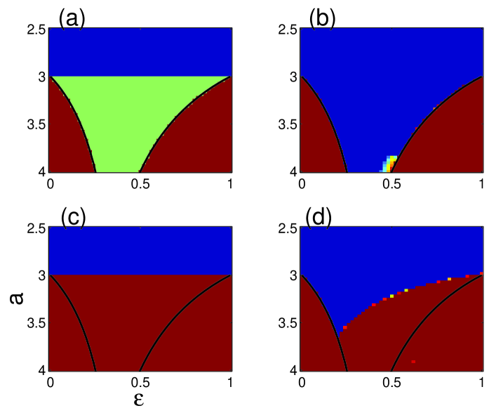
Figure 1: (a) Analytically calculated stability regions for the logistic map with one delay term. The trivial stability region defined by Eq. (14) is displayed in black (blue online), the instability regions defined by Eqs. (15) and (21) are displayed in dark grey (red online). (b)-(d) Stability regions calculated numerically, by simulation of Eq. (2) with one delay term and different initial conditions. The parameter regions where the fixed point is stable for all initial conditions are displayed in black (blue online). The black solid lines indicate the borders of the instability regions defined by Eqs.(15) and (21). Near these boundaries there is sensitivity to the initial conditions: some trajectories evolve towards the fixed point, while others evolve to periodic or chaotic orbits. The delay times are (b) $\tau_{1}=1$, (c) $\tau_{1}=2$, (d) $\tau_{1}=3$.

Additional information can be obtained by calculating explicitly the eigenvalues of $A$. The roots of the characteristic equation

$$\det\begin{pmatrix}(1-\epsilon)f^{\prime}(x_{0})+\alpha_{0}-\lambda&\alpha_{1}&\alpha_{2}&\ldots&\alpha_{M-1}&\alpha_{M}\\ 1&-\lambda&0&\ldots&0&0\\ 0&1&-\lambda&\ldots&0&0\\ \vdots&&&&\vdots\\ 0&0&0&\ldots&-\lambda&0\\ 0&0&0&\ldots&1&-\lambda\end{pmatrix}=0,$$ (16)

can be written in terms of the determinant of two $M\times M$ matrices:

$$[(1-\epsilon)f^{\prime}(x_{0})+\alpha_{0}-\lambda]\det C-\det B=0,$$ (17)

where

$$C=\begin{pmatrix}-\lambda&0&\ldots&0&0\\ 1&-\lambda&\ldots&0&0\\ \vdots&&&&\vdots\\ 0&0&\ldots&-\lambda&0\\ 0&0&\ldots&1&-\lambda\end{pmatrix}$$ (18)

and

$$B=\begin{pmatrix}\alpha_{1}&\alpha_{2}&\ldots&\alpha_{M-1}&\alpha_{M}\\ 1&-\lambda&\ldots&0&0\\ \vdots&&&&\vdots\\ 0&0&\ldots&-\lambda&0\\ 0&0&\ldots&1&-\lambda\end{pmatrix}.$$ (19)

We calculated the determinant of each matrix recursively (details are presented in the appendix) obtaining:

$$\lambda^{M+1}-[(1-\epsilon)f^{\prime}(x_{0})+\alpha_{0}]\lambda^{M}-\sum_{j=1}^{M}\alpha_{j}\lambda^{M-j}=0.$$ (20)

The roots of Eq.(20) satisfy $\prod_{i=0}^{M}|\lambda_{i}|=|\alpha_{M}|$. Thus, if

$$|\alpha_{M}|=|l_{M}\epsilon f^{\prime}(x_{0})/N|>1$$ (21)

at least one eigenvalue has $|\lambda|>1$, i.e., this gives another analytic (sufficient) instability condition. For $l_{M}/N=1$ Eq.(21) holds in the right-bottom corner of Fig. 1(a) (large $a$ , large $\epsilon$); for $l_{M}/N<1$ Eq.(21) is not satisfied in the parameter region of interest ($a$ $\in$ [0,4], $\epsilon$ $\in$ [0,1]). Notice that if $l_{M}/N=1$, then the map has only one feedback loop (because the multiplicity of the feedback terms with maximum delay is equal to the total number of feedback terms); therefore, Eq.(21) indicates that when a logistic map has a single feedback term, the fixed-point solution can not be stable in the parameter region (large $a$, large $\epsilon$), regardless of the delay time. In other words, a single feedback term can not stabilize the fixed point in the (large $a$, large $\epsilon$) parameter region. Numerical simulations of Eq.(2) with $N=1$ and different delays confirm these analytical predictions, see Figs. 1(b)-(d).

Further analytical insight can be gained by considering two special cases: all-even and all-odds delays. First, let us show that if the delays are all even (and therefore, $M$ is even), $\lambda=-1$ is a solution of Eq. (20) when $f^{\prime}(x_{0})=-1$, i.e., at the border of the stability region, Eq.(14). Substituting $\lambda=-1$ in Eq.(20) and taking into account that $M-j$ is even (since in the sum only terms with $j$ even are different from zero) gives

$$-1-[(1-\epsilon)f^{\prime}(x_{0})+\alpha_{0}]-\sum_{j=1}^{M}\alpha_{j}=0.$$ (22)

Using $\sum_{j=0}^{M}\alpha_{j}=\epsilon f^{\prime}(x_{0})$ we obtain $f^{\prime}(x_{0})=-1$. Therefore, when the delays are all-even there is an eigenvalue $\lambda=-1$ if and only if $a=3$, regardless of $\epsilon$.

Next, let’s see what happens if the delay times are all odd, therefore, $M$ is odd and, in addition, $\alpha_{0}=0$. Taking into account that $M-j$ is even (since in the sum only terms with $j$ odd are different from zero) for $\lambda=-1$ Eq. (20) gives

$$1+[(1-\epsilon)f^{\prime}(x_{0})]-\sum_{j=1}^{M}\alpha_{j}=0.$$ (23)

Using $\sum_{j=1}^{M}\alpha_{j}=\epsilon f^{\prime}(x_{0})$ we obtain $f^{\prime}(x_{0})=-1/(1-2\epsilon)$. For the logistic map this gives $a=(3-4\epsilon)/(1-2\epsilon)$ a condition which is satisfied for $\epsilon\in[0,1]$ only for values of $a$ inside the stability region $a<3$.

The above analysis allows as to draw some additional conclusions about the stability of the fixed point in the special cases of all-even and all-odd delays. For all-even delays an eigenvalue is real and negative and equal to $-1$ for $a=3$. For larger $a$ this eigenvalue can in principle become $\lambda<-1$ rendering the fixed point unstable due to a period-doubling bifurcation. For all-odd delays this instability scenario is not possible, as $\lambda=-1$ in a parameter region where we know that all eigenvalues must have $|\lambda|\leq 1$.

We verified these predictions by calculating numerically the eigenvalues of $A$. Figure 2 displays results for all-odd and all-even delays, varying $a$ while keeping $\epsilon$ constant. It can be observed that for all-even delays one real eigenvalue becomes less than $-1$ for $a>3$; for all-odd delays a pair of complex-conjugate eigenvalues have modulus greater than $1$ for $a>3.8$.

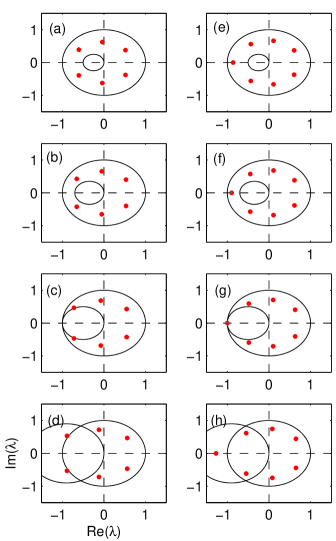
Figure 2: Eigenvalues in the complex plane for a map with $N=3$ feedback loops with all-odd delays (left column: $\tau_{j}=$1, 3, 5) and all-even delays (right column: $\tau_{j}=$2, 4, 6). $\epsilon=0.5$ and (a), (e) $a=2.5$; (b), (f) $a=2.7$; (c), (g) $a=3.0$ and (d), (h) $a=3.8$. The circles indicate the Gershgorin disks.

III Numerical Results

In this section we compare the dynamics of a logistic map with $N$ self-feedback loops, Eq. (2), with the dynamics of a map of an array of $N$ globally delayed-coupled logistic maps, Eq. (1).

We consider Gaussian distributed delays: $\tau_{ij}=\tau_{0}+\mathrm{Near}(c\xi)$, where $c$ is a parameter that allows varying the width of the delay distribution (for $c=0$ the delays are all equal, $\tau_{ij}=\tau_{0}$, for $c\neq 0$ the delays are distributed around $\tau_{0}$); $\xi$ is Gaussian distributed with zero mean and standard deviation one; $\mathrm{Near}$ denotes the nearest integer (we use $\mathrm{Near}$ instead of $\mathrm{Int}$ to have a distribution that is symmetric with respect to $\tau_{0}$; however, the results are largely independent of the precise form of the delay distribution). Depending on $\tau_{0}$ and $c$ the distribution of delays has to be truncated to avoid negative delays.

We begin by showing that if $N$ is large enough, the parameter region where the fixed point is stable for the array is remarkably similar to the parameter region where the fixed point is stable for the map with feedback loops. Figure 3 displays results for three values of $N$, the upper row shows the stability region of the homogeneous steady-state solution of the array [$x_{i}(t)=x_{j}(t)=x_{0}$ $\forall$ $i$, $j$, $t$], while the lower row shows the stability region of the fixed point solution the map with feedback loops. The delays of the self-feedback terms, $\tau_{j}$ with $j=1\dots N$, were taken equal to the delay times of the interaction of the $i$th and $j$th maps of the array; this gives $N$ sets of delay times ($\tau_{j}=\tau_{ij}$ with $i=1\dots N$). In the lower row of Fig. 3, the parameter region where the fixed point is stable for all sets of delays is displayed in black (blue online), and the regions where is unstable for all sets of delays are displayed in dark gray (red online). Outside the trivial stability region ($a\leq 3$) and outside the instability region defined by the sufficient condition Eq. (15), if $N$ is small the fixed point of the map with self-feedback loops can be stable or unstable depending on $\tau_{j}$ (i.e., the fixed point can be stable for the $i$th set of delays and not for the $k$th set of delays); however, if $N$ is sufficiently large the stability of the fixed point is the same for all sets of delays (there is sensitivity to the precise values of $\tau_{j}$ near the boundaries of the instability regions). It can be observed that for both, the single map and the array, the fixed point is unstable in the left-bottom corner (large $a$, low $\epsilon$), in agreement with the results of the previous section (where we showed that in this region the sufficient instability condition, Eq.(15), holds).

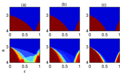
Figure 3: Stability region of the fixed point solution of an array of $N$ maps (upper row) and of a map with $N$ feedback loops (lower row). The delays are Gaussian distributed with $\tau_{0}=3$, $c=1$. The dynamics of the map with feedback loops was simulated for various sets of delays $\tau_{j}$: the fixed point was found to be stable for all sets in the black region (blue online) and unstable for all sets in the dark gray regions (red online). The solid line indicates the borders of the instability region defined by Eq. (15). (a) $N=10$, (b) $N=20$, (c) $N=100$.

The stability of the fixed point depends on the distribution of delays, and again, the similarities between a map of the array and a map with self-feedback loops, for $N$ large enough, are remarkable. As the width of the delay distribution, $c$, increases, the parameter region where the fixed point is stable grows (see Fig. 4), and this occurs for both, the array and the map with self-feedback loops.

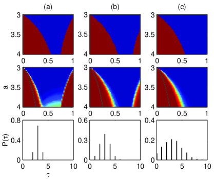
Figure 4: Influence of the width of the delay distribution on the stability of the fixed point solution of an array of $N$ maps (upper row) and of a map with $N$ feedback loops (middle row). The delays (lower row) are Gaussian distributed with $\tau_{0}=3$, (a) $c=0.5$, (b) $c=1$ , (c) $c=2$. $N=100$.

For the array of coupled maps, the parameter that quantifies the influence of the delays is not the mean delay, $<\tau>$, or the standard deviation of the distribution, $D_{\tau}$, but is the normalized disorder parameter, $c^{\ast}=D_{\tau}/<\tau>$ prl ($<\tau>=\tau_{0}$, $D_{\tau}=c$, and $c^{\ast}=c/\tau_{0}$ if the Gaussian distribution is not truncated). Figure 5 shows that this is also the case for the map with self-feedback loops, as it can be noticed that the stability region of the fixed point is the same for distributions that have different $<\tau>$ and $D_{\tau}$, but the same normalized width, $c^{\ast}$.

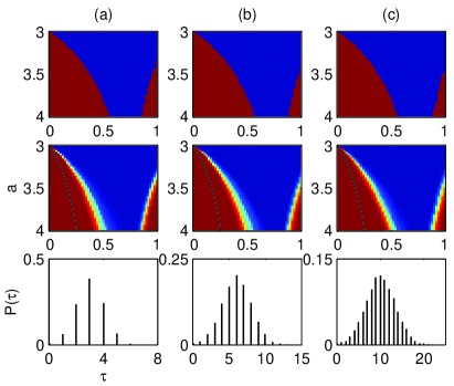
Figure 5: Influence of the normalized disorder parameter on the stability of the fixed point solution of an array of $N$ maps (upper row) and of a map with $N$ feedback loops (middle row). The delays (lower row) are Gaussian distributed with different mean and different standard deviation but with the same normalized width, $c^{\ast}\sim c/\tau_{0}$ (a) $\tau_{0}=3$, $c=1$, (b) $\tau_{0}=6$, $c=2$ , (c) $\tau_{0}=10$, $c=3.33$. $N=100$.

Figure 6(a) displays the stability region of the fixed point solution for the array (upper row) and for the map with self-feedback loops (lower row), in the parameter space [$\tau_{0}$ ($\sim<\tau>$), $c$ ($\sim D_{\tau}$)]. It can be observed that the fixed point is stable if the delays are random enough (i.e., if the width of the distribution, $c$, is larger than a certain value that increases with $\tau_{0}$). When the stability region is plotted vs. the normalized width, $c^{\ast}$ [Fig. 6(b)], it can be observed than the value of $c^{\ast}$ above which the fixed point is stable is independent of $\tau_{0}$ [but depends on $\epsilon$, as shown in Fig. 6(c)]. This occurs for both, the map of the array and the map with self-feedback loops.

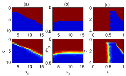
Figure 6: (a) Stability region of the fixed point solution of an array of $N$ maps (upper row) and of a map with $N$ feedback loops (lower row) in the parameter space (mean delay, standard deviation). (b) Same as (a) but plotted vs. the normalized disorder parameter, see text. (c) Same as (a) but in parameter space ($\epsilon$, disorder parameter). $N=100$, $a=4$, in (a),(b) $\epsilon=1$; in (c) $\tau_{0}=5$.

While the above observation of enhanced fixed-point stability with increasing randomness of delays is generic, independent of the precise form of the delay distribution, there is an exception which is the case of all-even delays. For all-even delays the fixed point of the map with self-feedback terms is stable only in the region defined by the sufficient trivial stability condition, Eq.(14). Because the fixed point becomes unstable due to a period-doubling bifurcation when one real eigenvalue becomes $\lambda<-1$ (as discussed in the previous section), all-even delays tend to stabilize an orbit of period 2. The same effect is observed in the array of $N$ logistic maps: for all even delays the fixed point is stable only in the trivial region $a\leq 3$.

If $N$ is sufficiently large, a map with $N$ self-feedback loops and a map of an array of $N$ maps follow very similar instabilities scenarios when $\epsilon$ or $a$ are varied (see below for a discussion of the limit in which the similarities are not only qualitative but also quantitative). As an example, Figs. 7-9 display bifurcation diagrams for varying $\epsilon$ while keeping $a$ fixed. The delays are “mixed” (even and odd) in Fig. 7, all-odd in Fig. 8, and all-even in Fig. 9. The parameters correspond to a scan of $\epsilon$ along the horizontal axis of Fig. 4(b): for “mixed” delays the fixed point is stable in a range of $\epsilon$ for both, the map with feedback loops and the array. Figures 7(a)-9(a) [7(b)-9(b)] display the time evolution of one element of the array, $i=1$ ($i=2$), by plotting 100 consecutive interactions of $x_{1}$ ($x_{2}$) after transients die away vs. $\epsilon$. Figures 7(c)-9(c) display the array configuration at time $t=T$ (large enough to let transients die away). Figures 7(d)-9(d) [7(e)-9(e)] display the time evolution of the map with feedback loops with delays $\tau_{j}=\tau_{1j}$ ($\tau_{j}=\tau_{2j}$), by plotting 100 consecutive interactions of $x$ (after transients die away) vs. $\epsilon$.

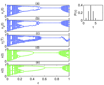
Figure 7: Bifurcation diagrams for increasing $\epsilon$. (a) $i=1$ map of the array. (b) $i=2$ map of the array. (c) Array configuration, $x_{i}$ with $i=1,\dots,N$ at time $t=T$. (d) A map with feedback loops with delays $\tau_{j}=\tau_{1j}$. (e) A map with feedback loops with delays $\tau_{j}=\tau_{2j}$. $a=4$, $N=100$, the delays are Gaussian distributed with $\tau_{0}=3$, $c=1$.

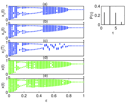
Figure 8: As Fig. 7 but with all-odd delays.

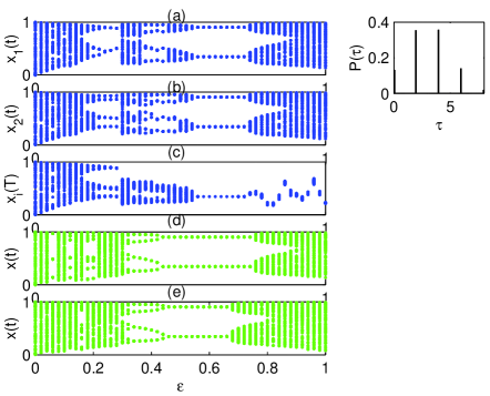
Figure 9: As Fig. 7 but with all-even delays.

Above a certain coupling strength the array synchronizes in a single cluster that displays either steady-state or time-dependent dynamics [in Figs. 7(c)-9(c) there is a single cloud of points for $\epsilon>\approx 0.5$]; below this coupling strength the array splits into clusters and the elements of each cluster evolve along similar time-dependent orbits (the bifurcation diagrams for the elements $i=1$ and $i=2$ of the array are similar, even for low $\epsilon$).

For a map with self-feedback loops with “mixed” delays, the fixed point is stabilized for increasing $\epsilon$ after a period-doubling bifurcation [Fig. 7(d),(e)]. In contrast, for feedback loops with all-odd delays the fixed point is stabilized after a Hopf bifurcation [Fig. 8(d),(e)]. For all-even delays the fixed point is not stable for any $\epsilon$ [but the period-two orbit is stable in a certain range of $\epsilon$, Fig. 9(d),(e)]. These results are in agreement with the analysis of the previous section, where we found that for all-odd delays the fixed point changes stability when a pair of complex eigenvalues cross the unit circle, and for all-even delays the fixed point changes stability when a real eigenvalue crosses the unit circle at $\lambda=-1$. The bifurcation diagrams of the $i=1$ and $i=2$ maps of the array display similar features [Figs. 7-9(a), 7-9(b)]: the fixed point is stable in a range of $\epsilon$ for “mixed” and all-odd delays, while the period-two orbit is stable in a range of $\epsilon$ in the case of all-even delays.

Exponentially distributed delays [$\tau_{ij}=\tau_{0}+\mathrm{Int}(c\xi)$, where $\xi$ is exponentially distributed, positive, with unit mean] yield similar bifurcation diagrams, shown in Fig. 10. Furthermore, the instability scenario for fixed $\epsilon$ and increasing $a$ (i.e., a scan along a vertical line in Fig. 4) is also very similar, as shown in Fig. 11.

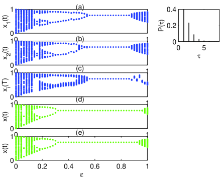
Figure 10: As Fig. 7 but with exponentially distributed delays ($\tau_{0}=1$, $c=1$).

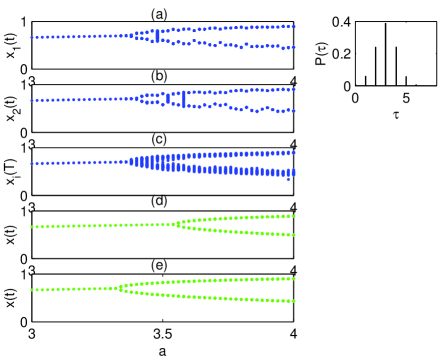
Figure 11: As Fig. 7 but varying $a$ while keeping $\epsilon=0.3$ fixed.

IV Discussion

The similarities between a map of the array and a map with self-feedback loops can be interpreted in the framework of the analogy between globally coupled maps (with instantaneous coupling), and a single map subjected to an external drive, studied by Cosenza and Parravano in Refs.cosenza1 ; cosenza2 . The authors considered

$$x_{i}(t+1)=(1-\epsilon)f[x_{i}(t)]+\epsilon H(x_{1}(t)\dots x_{N}(t)),$$ (24)

where $H$ is a global coupling function that is invariant to argument permutations [$H(x_{1},\dots,x_{i},\dots,x_{j},\dots x_{N})=H(x_{1},\dots,x_{j},\dots,x_{i},\dots,x_{N})$ $\forall$ $i$ and $j$], and showed that the clustering behavior of the array can be analyzed through the analogy with the driven map,

$$x(t+1)=(1-\epsilon)f[x(t)]+\epsilon F(t),$$ (25)

where $F(t)$ is a external forcing (assumed to be periodic). The analogy holds because in Eq.(24) all the elements of the array are affected by the coupling function $H$ in exactly the same way at all times, and therefore the behavior of any element of the array is equivalent to the behavior of the driven map, Eq. (25).

To analyze whether this analogy can be extended to the case of delayed-coupling, we calculated the mean field coupling term at site $i$ of the array,

$$H_{i}(t)=\frac{1}{N}\sum_{j=1}^{N}f[x_{j}(t-\tau_{ij})],$$ (26)

and compared with the driving term of the map,

$$F(t)=\frac{1}{N}\sum_{j=1}^{N}f[x(t-\tau_{j})].$$ (27)

We found that for $N$ large, $H_{i}(t)$ is nearly the same for all the elements of the array, regardless of the array dynamics, and its time evolution is similar to that of the driving term of the map, $F$. As an example, Fig. 12 displays the mean field coupling term and the driving term, for parameters corresponding to the bifurcation diagrams shown in Fig. 7. In Fig. 12(a) we plot 100 consecutive values of the mean field at one element of the array, $H_{1}$ (after transients die away). Figure 12(b) displays the mean field at all elements, $H_{i}$ with $i=1\dots N$, at time $t=T$ (large enough to let transients die away). It can be seen that $H_{i}\simeq H_{j}$ even for low values of $\epsilon$. Figure 12(c) displays 100 consecutive values of the driving term of the map with feedback loops, $F(t)$ (after transients die away), and it is observed that above a certain value of $\epsilon$ ($\epsilon\approx 0.2$) $F\simeq H_{1}$.

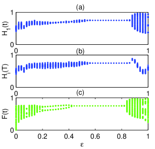
Figure 12: (a) Mean field for the $i=1$ map of the array vs. $\epsilon$. (b) Mean field for each map of the array, $H_{i}$ with $i=1\dots N$, vs. $\epsilon$. (c) Driving term of the map with feedback loops, $F$, vs. $\epsilon$. $N=100$, $a=4$, the delays are the same as in Fig. 7.

We speculate that the analogy with the single map has its roots in the fact that the elements of the array display similar temporal variation, i.e., they evolve along equal (or similar) orbits, even when the array splits into clusters. Therefore, a map of the array ”perceives” signals coming from other maps as nearly indistinguishable from signals coming from self-feedback loops. This can also be thought as an ergodic property of the dynamics, since the average over the ensemble, $H_{i}$, is nearly equal to the average over time, $F$.

The analogy holds even if the delays are all equal, $c=0$, as shown in Fig. 13. Above a certain coupling strength ($\epsilon\approx 0.45$) the array synchronizes in-phase, $x_{i}(t)=x_{j}(t)$ $\forall$ $i$, $j$, and therefore the analogy is mathematically trivial since in the synchronization manifold the evolution equation of one element of the array and the evolution equation for a map with a single self-feedback loop are exactly the same. However, multistability in the delayed map (i.e., the coexistence of different stable orbits) might lead to competition phenomena in the array of coupled maps, as different elements might tend to evolve along different orbits, depending on the initial conditions. The investigation of this type of dynamics is the object of future work.

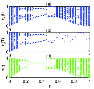
Figure 13: As Fig. 7 but with fixed delays ($\tau_{0}=1$, $c=0$).

V Summary and Conclusions

We investigated the dynamics of mutually coupled logistic maps focusing on the influence of the delay times of the interactions between the maps, and comparing with the dynamics of a map with several time-delayed self-feedback loops. By using some mathematical tools such as the Gershgorin theorem we derived analytic stability and instability conditions for the fixed point solution of the map with feedback loops. We found that the stabilization of the array in the fixed-point solution can be well understood in terms of the dynamics of the map. Specifically, for randomly distributed delay times, if $N$ and $\epsilon$ are large enough the fixed-point is stable for both, the map with self-feedback loops and the array. Also, if the delay times are all even, for both, the single map with $N$ delayed loops and the array of $N$ delayed-coupled maps, we observed that the stability region of the fixed-point is reduced to the “trivial” region ($a\leq 3$) regardless of the coupling strength. The results presented here provide another example of an ensemble of mutually coupled interacting units, where understanding the dynamics of a single unit with self-feedback loops is relevant for understanding the macroscopic behavior of the ensemble.

VI Acknowledgments

CM acknowledges support from the “Ramon and Cajal” Program (MCyT of Spain).

VII Appendix

In this appendix we demonstrate Eq. (20). We start from Eq. (17),

$$[(1-\epsilon)f^{\prime}(x_{0})+\alpha_{0}-\lambda]\det C-\det B=0,$$ (28)

and calculate the determinant of matrix $C$ recursively:

$$\det C=\det\begin{pmatrix}-\lambda&0&0&\ldots&0&0\\ 1&-\lambda&0&\ldots&0&0\\ 0&1&-\lambda&\ldots&0&0\\ \vdots&&&&\vdots\\ 0&0&0&\ldots&-\lambda&0\\ 0&0&0&\ldots&1&-\lambda\end{pmatrix}$$

$$=-\lambda\det\begin{pmatrix}-\lambda&0&\ldots&0&0\\ 1&-\lambda&\ldots&0&0\\ \vdots&&&&\vdots\\ 0&0&\ldots&-\lambda&0\\ 0&0&\ldots&1&-\lambda\end{pmatrix}$$

$$-\det\begin{pmatrix}0&0&\ldots&0&0\\ 1&-\lambda&\ldots&0&0\\ \vdots&&&&\vdots\\ 0&0&\ldots&-\lambda&0\\ 0&0&\ldots&1&-\lambda\end{pmatrix}$$ (29)

The second determinant is zero because the elements of the first row are all zero. We obtain

$$\det C(M)=-\lambda\det C(M-1)=\dots=(-\lambda)^{M}.$$ (30)

The determinant of matrix $B$ can also be calculated recursively:

$$\det B=\det\begin{pmatrix}\alpha_{1}&\alpha_{2}&\alpha_{3}&\ldots&\alpha_{M-1}&\alpha_{M}\\ 1&-\lambda&0&\ldots&0&0\\ 0&1&-\lambda&\ldots&0&0\\ \vdots&&&&\vdots\\ 0&0&0&\ldots&-\lambda&0\\ 0&0&0&\ldots&1&-\lambda\end{pmatrix}$$

$$=\alpha_{1}\det\begin{pmatrix}-\lambda&0&\ldots&0&0\\ 1&-\lambda&\ldots&0&0\\ \vdots&&&&\vdots\\ 0&0&\ldots&-\lambda&0\\ 0&0&\ldots&1&-\lambda\end{pmatrix}$$

$$-\det\begin{pmatrix}\alpha_{2}&\alpha_{3}&\ldots&\alpha_{M-1}&\alpha_{M}\\ 1&-\lambda&\ldots&0&0\\ \vdots&&&&\vdots\\ 0&0&\ldots&-\lambda&0\\ 0&0&\ldots&1&-\lambda\end{pmatrix}$$ (31)

It can be noticed that the first matrix is $C(M-1)$ while the determinant of the second matrix can be calculated recursively,

$$\det B(M)=\alpha_{1}\det C(M-1)-\det B(M-1),$$ (32)

where

$$B(M-1)=\begin{pmatrix}\alpha_{2}&\ldots&\alpha_{M-1}&\alpha_{M}\\ \vdots&&&\vdots\\ 0&\ldots&-\lambda&0\\ 0&\ldots&1&-\lambda\end{pmatrix}.$$ (33)

Substituting in (28)

$$[(1-\epsilon)f^{\prime}(x_{0})+\alpha_{0} - \lambda]\det C(M)-[\alpha_{1}\det C(M-1)$$

$$-\alpha_{2}\det C(M-2) + \det B(M-2)]=0$$ (34)

Using Eqs.(30) and(32) we obtain

$$[(1-\epsilon)f^{\prime}(x_{0})+\alpha_{0} - \lambda](-\lambda)^{M}-\alpha_{1}(-\lambda)^{M-1}$$

$$+\alpha_{2}(-\lambda)^{M-2} - \dots=0$$ (35)

which gives

$$(-\lambda)^{M+1}+[(1-\epsilon)f^{\prime}(x_{0})+\alpha_{0}](-\lambda)^{M}$$

$$+\sum_{j=1}^{M}(-1)^{j}\alpha_{j}(-\lambda)^{M-j}=0,$$ (36)

that can be simplified to

$$-\lambda^{M+1}+[(1-\epsilon)f^{\prime}(x_{0})+\alpha_{0}]\lambda^{M}+\sum_{j=1}^{M}\alpha_{j}\lambda^{M-j}=0.$$ (37)

References

- (1) A.S. Pikovsky, M.G. Rosenblum, and J. Kurths, Synchronization-A Universal Concept in Nonlinear Sciences (Cambridge University Press, Cambridge, England, 2001).
- (2) K. Kaneko, Phys. Rev. Lett. 63, 219 (1989); K. Kaneko, I. Tsuda, Complex Systems: Chaos and Beyond, A Constructive Approach with Applications in Life Sciences (Springer-Verlag, Berlin, Heidelberg, New York, 2000).
- (3) M. C. Mackey and L. Glass, Science 197, 287 (1977).
- (4) K. Ikeda, Opt. Commun. 30, 257 (1979).
- (5) J. Foss, A. Longtin, B. Mensour, and J. Milton, Phys. Rev. Lett. 76, 708 (1996) .
- (6) M. K. Stephen Yeung and S. H. Strogatz, Phys. Rev. Lett. 82, 648 (1999).
- (7) D. V. Ramana Reddy, A. Sen, and G. L. Johnston, Phys. Rev. Lett. 80, 5109 (1998).
- (8) K. Pyragas, Phys. Lett. A 170, 421 (1992).
- (9) D. Goldobin, M. Rosenblum, A. Pikovsky, Phys. Rev. E 67, 061119 (2003).
- (10) S. Boccaletti, E. Allaria, R. Meucci, Phys. Rev. E 69, 066211 (2004).
- (11) N. B. Janson, A.G. Balanov, E. Scholl, Phys. Rev. Lett. 93, 010601 (2004); A. G. Balanov et al., Physica D 199, 1 (2004).
- (12) K. Otsuka and J-L. Chern, Phys. Rev. A 45, 5052 (1992).
- (13) F. M. Atay, Phys. Rev. Lett. 91, 094101 (2003).
- (14) D. Huber and L. S. Tsimring, Phys. Rev. E 71, 036150 (2005).
- (15) C. W. Eurich, A. Thiel, and L. Fahse, Phys. Rev. Lett. 94, 158104 (2005).
- (16) C. Masoller and A. C. Marti, Phys. Rev. Lett. 94, 134102 (2005).
- (17) F. M. Atay, J. Jost and A. Wende, Phys. Rev. Lett. 92, 144101 (2004).
- (18) A. C. Marti and C. Masoller, Phys. Rev. E 67, 056219 (2003); C. Masoller, A. C. Marti and D. H. Zanette, Physica A 325, 186 (2003); A. C. Marti and C. Masoller, Physica A 342, 344 (2004).
- (19) A. Ahlborn and U. Parlitz, Phys. Rev. Lett. 93, 264101 (2004); Phys. Rev. E 72 016206 (2005).
- (20) A. Parravano and M. G. Cosenza, Phys. Rev. E 58 1665 (1998).
- (21) M. G. Cosenza and A. Parravano, Phys. Rev. E 64 036224 (2001).
- (22) J. Stoer and R. Burlisch, Introduction to Numerical Analysis (Springer, Berlin, 1992); P.A. Horn and C.R. Jonhson, Matrix Analysis (Cambridge University Press, New York, 1985). For a recent application of the Gershgorin theorem see: M. Timme et al., Phys. Rev. Lett. 92, 074101 (2004).