SYNCHRONIZATION OF SPECTRAL COMPONENTS
AND ITS REGULARITIES IN CHAOTIC DYNAMICAL SYSTEMS

Abstract

The chaotic synchronization regime in coupled dynamical systems is considered. It has been shown, that the onset of synchronous regime is based on the appearance of the phase relation between interacting chaotic oscillators frequency components of Fourier spectra. The criterion of synchronization of spectral components as well as the measure of synchronization have been discussed. The universal power law has been described. The main results are illustrated by coupled Rössler systems, Van-der-Pol and Van-der-Pol–Duffing oscillators.

Introduction

Chaotic synchronization is one of the fundamental phenomena actively studied last time  A. Pikovsky, M. Rosenblum, J. Kurths (2001), having important both theoretical and applied significance (e.g., for the information transmission by means of deterministic chaotic signals K. Murali, M. Lakshmanan (1994a); T. Yang T., C.W. Wu and L.O. Chua (1997), in biological R.C. Elson, A.I. Selverston, R. Huerta, N.F. Rulkov, M.I. Rabinovich, H.D.I. Abarbanel (1998) and physiological M.D. Prokhorov, V.I. Ponomarenko, V.I. Gridnev, M.B. Bodrov, A.B. Bespyatov (2003) tasks, etc.). Several different types of chaotic synchronization of coupled oscillators, i.e. generalized synchronization N.F. Rulkov, M.M. Sushchik, L.S. Tsimring, H.D.I. Abarbanel (1995), phase synchronization A. Pikovsky, M. Rosenblum, J. Kurths (2001), lag synchronization M.G. Rosenblum, A.S. Pikovsky, J. Kurths (1997) and complete synchronization L.M. Pecora, T.L. Carroll (1991) are traditionally distinguished. There are also attempts to find a unifying framework for chaotic synchronization of coupled dynamical systems R. Brown, L. Kocarev (2000); S. Boccaletti, J. Kurths, G. Osipov, D.L. Valladares, C.S. Zhou (2002); S. Boccaletti., L.M. Pecora, A. Pelaez (2001).

In our works A.E. Hramov, A.A. Koronovskii (2004); A.A. Koronovskii, A.E. Hramov (2004) it was shown that phase, generalized, lag and complete synchronization are closely connected with each other and, as a matter of fact, they are different manifestations of one type of synchronous oscillations behavior of coupled chaotic oscillators called time scale synchronization. Synchronous regime character (phase, generalized, lag or complete synchronization) is defined by the presence of synchronous time scales $s$, introduced by means of continuous wavelet transform B. Torresani (1995); I. Daubechies (1992); A.A. Koronovskii, A.E. Hramov (2003) with Molrlet mother wavelet function. Each of time scales can be characterized by the phase $\phi_{s}(t)=\arg W(s,t)$, where $W(s,t)$ is the complex wavelet surface. In this case, the phenomenon of chaotic synchronization of coupled systems is manifested by a synchronous behavior of the phases of coupled chaotic oscillators $\phi_{s1,2}(t)$ observed on certain synchronized time scales range $s_{m}<s<s_{b}$, for time scales $s$ from which the phase locking condition

$$|\phi_{s1}(t)-\phi_{s2}(t)|<\mathrm{const}$$ (1)

is satisfied, and the part of the wavelet spectrum energy being fallen on this range does not equal zero (see A.E. Hramov, A.A. Koronovskii (2004); A.E. Hramov, A.A. Koronovskii, P.V. Popov, I.S. Rempen (2005) for detail). The range of synchronized time scales $[s_{m};s_{b}]$ expands when the coupling parameter between systems increases. If the coupling type between oscillators is defined in such a way that the lag synchronization appearance is possible then all time scales become synchronized with further coupling parameter increasing, while the coinciding states of interacting oscillators are shifted in time relative to each other: $\mathbf{x}_{1}(t-\tau)\simeq\mathbf{x}_{2}(t)$. Further coupling parameter increasing leads to a decrease of the time shift $\tau$. The oscillators tend to the regime of complete synchronization, $\mathbf{x}_{1}(t)\simeq\mathbf{x}_{2}(t)$ and the phase difference $(\phi_{s1}(t)-\phi_{s2}(t))$ tends to be zero on all time scales.

The time scale $s$ introduced into consideration by means of continuous wavelet transform can be considered as a quantity which is inversely proportional to the frequency $f$ defined with the help of Fourier transformation. For the Morlet mother wavelet function I. Daubechies (1992) with parameter $\Omega=2\pi$ the relationship between the frequency $f$ and the time scale is quite simple: $s=1/f$. Therefore, the time scale synchronization should also manifest in the appearance of the phase relation between frequency components $f$ of corresponding Fourier spectra $S(f)$ of interacting oscillators.

In this paper we consider the synchronization of spectral components of Fourier spectra of coupled oscillators. We discuss the mechanism of chaotic synchronization regime manifestation in coupled dynamical systems based on the appearance of the phase relation between frequency components of Fourier spectra of interacting chaotic oscillators (see also N.F. Rulkov, A.R. Volkovskii, A. Rodriguez-Lozano, E. Del Rio and M.G.Velarde (1994)). One can also consider the obtained results as a criterion of existence (or otherwise, an impossibility of existence) of lag synchronization regime in coupled dynamical systems.

The structure of this paper is the following. In Section I we discuss the synchronization of spectral components of Fourier spectra. We illustrate our approach with the help of two coupled Rössler systems in Sec. II. The quantitative measure of synchronization is described in Section III. The universal power law taking place in the presence of time scale synchronization regime is discussed in Sections IV and V. The final conclusion is presented in Section VI.

I Synchronization of spectral components of Fourier spectra

It should be noted that the continuous wavelet transform is characterized by the frequency resolution lower than the Fourier transformation (see I. Daubechies (1992); A.A. Koronovskii, A.E. Hramov (2003)). The continuous wavelet transform appears as smoothing of the Fourier spectrum, whereby the dynamics on a time scale $s$ is determined not only by the spectral component $f=1/s$ of the Fourier spectrum. This dynamics is also influenced by the neighboring components as well, the degree of this influence depends both on their positions in the Fourier spectrum and on their intensities. Thus, the fact that coupled chaotic oscillators exhibit synchronization on a time scale $s$ of the wavelet spectrum by no means implies that the corresponding components $f=1/s$ of the Fourier spectrum of these systems are also synchronized.

Let $x_{1}(t)$ and $x_{2}(t)$ be the time series generated by the first and the second coupled chaotic oscillators, respectively. The corresponding Fourier spectra are determined by the relations

$$S_{1,2}(f)=\int\limits_{-\infty}^{+\infty}x_{1,2}(t)e^{-i2\pi ft}\,dt.$$ (2)

Accordingly, each spectral component $f$ of the Fourier spectrum $S(f)$ can be characterized by an instantaneous phase $\phi_{f}(t)=\phi_{f0}+2\pi ft$, where ${\phi_{f0}=\arg S(f)}$. However, since the phase $\phi_{f}(t)$ corresponding to the frequency $f$ of the Fourier spectrum $S(f)$ increases with the time linearly, the phase difference of the interacting oscillators at this frequency ${\phi_{f1}(t)-\phi_{f2}(t)}={\phi_{f01}-\phi_{f02}}$ is always bounded and, hence, the traditional condition of phase entrainment (used for detection of the phase synchronization regime)

$$|\phi_{1}(t)-\phi_{2}(t)|<\mathrm{const},$$ (3)

is useless. Apparently, a different criterion should be used to detect the synchronization of coupled oscillators at a given frequency $f$.

In the regime of lag synchronization, the behavior of coupled oscillators is synchronized on all time scales $s$ of the wavelet transform (see A.E. Hramov, A.A. Koronovskii (2004)). Therefore, one can expect that all frequency components of the Fourier spectra of the systems under consideration should be synchronized as well. In this case, $x_{1}(t-\tau)\simeq x_{2}(t)$ and, hence, taking into account (2) one has to obtain

$$S_{2}(f)\simeq S_{1}(f)e^{i2\pi\tau f}.$$ (4)

Thus, in the case of coupled chaotic oscillators occurring in the regime of lag synchronization their instantaneous phases corresponding to the spectral component $f$ of the Fourier spectra $S_{1,2}(f)$ will be related to each other as ${\phi_{f2}(t)\simeq\phi_{f1}(t)+2\pi\tau f}$ and, hence, the phase difference $\phi_{f2}(t)-\phi_{f1}(t)$ of coupled oscillators on the frequency $f$ must obey the relation

$$\begin{split}\Delta\phi_{f}&=\phi_{f1}(t)-\phi_{f2}(t)=\\ &=\phi_{f01}-\phi_{f02}=2\pi\tau f.\end{split}$$ (5)

Accordingly, the points corresponding to the phase difference $\Delta\varphi_{f}$ of the spectral components of chaotic oscillators in the regime of lag synchronization on the $(f,\Delta\phi_{f})$ plane must fit a straight line with slope $k=2\pi\tau$. In the case of complete synchronization of two coupled identical oscillators the slope of this line $k$ is equal to zero (see also V.S. Anishchenko, T.E. Vadivasova, D.E. Postnov, M.A. Safonova (1992)).

The destroying of the lag synchronization regime (e.g., as a result of decrease of the coupling strength between oscillators) and transition to the regime of phase synchronization (in the case when the instantaneous phase of chaotic signal can be introduced correctly V.S. Anishchenko, T.E. Vadivasova (2004)) results in the loss of synchronism for a part of time scales $s$ of the wavelet spectra A.E. Hramov, A.A. Koronovskii (2004). Accordingly, one can expect that a part of spectral components of the Fourier spectra in the phase synchronization regime will also lose synchronism and the points on the $(f,\Delta\phi_{f})$ plane will deviate from the straight line (5) mentioned above . It is reasonable to assume that synchronism will be lost primarily for the spectral components $f$ characterized by a small fraction of energy in the Fourier spectra $S_{1,2}(f)$, while the components corresponding to a greater energy fraction will remain synchronized and the corresponding points on the $(f,\Delta\phi_{f})$ plane will be located at the straight line as before. As the lag synchronization regime does not occur in the system any more, the time shift $\tau$ can be determined by the delay of the most energetic frequency component $f_{m}$ in the Fourier spectra ${\tau=(\phi_{f_{m}2}-\phi_{f_{m}1})/(2\pi f_{m})}$.

As the coupling parameter decreases further, an increasing part of the spectral components will deviate from synchronism. However, as long as the most “energetic” components remain synchronized, the coupled systems will exhibit the regime of time scale synchronization. Obviously, that for the synchronized spectral component the phase difference $\Delta\varphi_{f}$ is located after the transient finished independently on initial conditions.

To describe the synchronization of spectral components, let us introduce a quantitative characteristic of a number of spectral components of the Fourier spectra $S_{1,2}(f)$ occurring in the regime of synchronism,

$$\sigma_{L}=\\ \frac{\int\limits_{0}^{+\infty}H(|S_{1}(f)|^{2}-L)H(|S_{2}(f)|^{2}-L)\left(\Delta\phi_{f}-2\pi\tau f\right)^{2}\,df}{\int\limits_{0}^{+\infty}H(|S_{1}(f)|^{2}-L)H(|S_{2}(f)|^{2}-L)\,df},$$ (6)

where $H(\xi)$ is the Heaviside function, $L$ is the threshold power level (in dB) above which the spectral components are taken into account, and $\tau$ is determined by the time shift of the most energetic frequency component ($f_{m}$) in the Fourier spectra, ${\tau=(\phi_{f_{m}2}-\phi_{f_{m}1})/(2\pi f_{m})}$. The quantity $\sigma_{L}$ tends to be zero in the regimes of complete and lag synchronization. After the lag synchronization regime destroying caused by the decrease of the coupling strength the value of $\sigma_{L}$ increases with the number of desynchronized spectral component of the Fourier spectra $S_{1,2}(f)$ of coupled oscillators.

Real data are usually represented by discrete time series of a finite length. In such cases, the continuous Fourier transform (2) has to be replaced by its discrete analog (as it was done in V.S. Anishchenko, T.E. Vadivasova, D.E. Postnov, M.A. Safonova (1992)), and the integral (6), by the sum

$$\sigma_{L}=\frac{1}{N}\sum\limits_{j=1}^{N}\left(\Delta\phi_{f_{j}}-2\pi\tau f_{j}\right)^{2},$$ (7)

taken over all spectral components of the Fourier spectra $S_{1,2}(f)$ with the power above $L$. In calculating $\sigma_{L}$, it is expedient to perform averaging over a set of time series $x_{1,2}(t)$. The phase shift $\Delta\varphi_{f}$ can be calculated either in the way as it was done in V.S. Anishchenko, T.E. Vadivasova, D.E. Postnov, M.A. Safonova (1992) or by means of cross spectrum I. Noda, Y. Ozaki (2002).

II Two mutually coupled Rössler systems synchronization

In order to illustrate the approach proposed above, let us consider two coupled Rössler systems

$$\begin{split}&\dot{x}_{1,2}=-\omega_{1,2}y_{1,2}-z_{1,2}+\varepsilon(x_{2,1}-x_{1,2}),\\ &\dot{y}_{1,2}=\omega_{1,2}x_{1,2}+ay_{1,2}+\varepsilon(y_{2,1}-y_{1,2}),\\ &\dot{z}_{1,2}=p+z_{1,2}(x_{1,2}-c),\end{split}$$ (8)

where $\varepsilon$ is the coupling parameter, ${\omega_{1}=0.98}$, ${\omega_{2}=1.03}$. By analogy with the case studied in M.G. Rosenblum, A.S. Pikovsky, J. Kurths, G.V. Osipov, I.Z. Kiss, J.L. Hudson (2002), the values of control parameters have been selected as follows: ${a=0.22}$, ${p=0.1}$ and ${c=8.5}$. It is known M.G. Rosenblum, A.S. Pikovsky, J. Kurths, G.V. Osipov, I.Z. Kiss, J.L. Hudson (2002) that two coupled Rössler systems with $\varepsilon=0.05$ occur in the regime of phase synchronization, while for $\varepsilon=0.15$ the same systems exhibit lag synchronization.

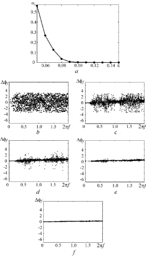
Figure 1: (a) The value $\sigma_{L}$ versus coupling parameter $\varepsilon$ and (b)–(f) the phase difference $\Delta\varphi_{f}$ of various spectral components $f$ of the Fourier spectra $S_{1,2}(f)$ of two coupled Rössler systems for different values of coupling strength $\varepsilon$. (b) The asynchronous dynamics for coupling parameter $\varepsilon=0.02$; (c) The chaotic synchronization regime $\varepsilon=0.05$; (d), $\varepsilon=0.08$; (e) $\varepsilon=0.1$ and (f) $\varepsilon=0.15$. The plots are constructed for the time series $x_{1,2}(t)$ with a length of 2000 dimensionless time units at a discretization step of $h=0.2$ at a power level of $L=-40$ dB of Fourier spectra $S_{1,2}(f)$

Figure 1,a shows a plot of the value $\sigma_{L}$ versus coupling parameter $\varepsilon$. One can see that $\sigma_{L}$ tends to be zero when the coupling parameter $\varepsilon$ increases, which is the evidence of the transition from phase to lag synchronization. Figures 1,b–1,f illustrate the increase in the number of synchronized spectral components of the Fourier spectra $S_{1,2}(f)$ of two coupled systems with coupling strength $\varepsilon$ increasing. Indeed, Fig. 1,b corresponds to the asynchronous dynamics of coupled oscillators ($\varepsilon=0.02$). There are no synchronous spectral components for such coupling strength and dots are scattered randomly over the $(f,\Delta\phi_{f})$ plane. The weak phase synchronization ($\varepsilon=0.05$) after the regime occurence is shown in the Fig. 1,c. There are a few synchronized spectral components the phase shift $\Delta\varphi_{f}$ of which satisfies the condition (5). Almost all spectral components are non-synchronized, therefore the points corresponding to the phase differences $\Delta\varphi_{f}$ are spread over $(f,\Delta\phi_{f})$ plane and the value of $\sigma_{L}$ is rather large.

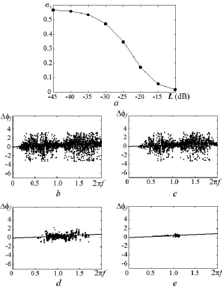
Figure 2: (a) The value $\sigma_{L}$ versus power $L$ at which the spectral components $f_{j}$ of the Fourier spectra $S_{1,2}(f)$ are taken into account in equation (7). (b)–(e) The phase difference $\Delta\varphi_{f}$ of various spectral components $f$ of the Fourier spectra $S_{1,2}(f)$ of two coupled Rössler systems for various power levels $L=-40$ dB (b), $L=-30$ dB (c), $L=-20$ dB (d) and $L=-10$ dB (e) for coupling strength $\varepsilon=0.05$

Figures 1,d and 1, e correspond to the well pronounced phase synchronization ($\varepsilon=0.08$ and $0.1$, respectively). Fig. 1,f shows the state of lag synchronization ($\varepsilon=0.15$), when all spectral components $f$ of Fourier spectra are synchronized. Accordingly, in this case all points on the $(f,\Delta\phi_{f})$ plane are at the line (5) with slope $k=2\pi\tau$. With coupling strength $\varepsilon$ increasing, the value of $\sigma_{L}$ decreases monotonically that verifies the assumption that when two coupled chaotic systems undergo transition from asynchronous dynamics to lag synchronization, more and more spectral components become synchronized. When all spectral components $f$ are synchronized, the phase shift $\Delta\varphi_{f}$ for them is $2\pi\tau f$, therefore the points on the $(f,\Delta\phi_{f})$ plane lie on the straight line (5) and the value of $\sigma_{L}$ is equal to zero.

Another important question is which spectral components of the Fourier spectra of interacting chaotic oscillators are synchronized first and which do it last. Figure 2,a shows a plot of the $\sigma_{L}$ value for the coupling strength $\varepsilon=0.05$ (corresponding to the weak phase synchronization) versus power $L$ at which the spectral components $f_{j}$ of the Fourier spectra $S_{1,2}(f)$ are taken into account in equation (7). One can see that the “truncation” of the spectral components with small energy leads to a decrease of the $\sigma_{L}$ value. Figures 1,b–1,e illustrate the distribution of the phase difference $\Delta\varphi_{f}$ of the spectral components $f$ with the power exceeding the preset level $L$. The data in Fig. 2 show that the most “energetic” spectral components are first synchronized upon the onset of time scale synchronization. On the contrary, the components with low energies are the first to go out from synchronism upon destroying of the lag synchronization regime.

III A criterion and measure of synchronization

Let us briefly discuss a criterion of spectral components synchronization. Obviously, the relation (5) is quite convenient as a criterion of synchronism in case of lag synchronization destroying in the way considered above. If the type of coupling between systems has been defined in such a manner that the lag synchronization regime can not appear, the relation (5) can not be the criterion of spectral components synchronization. So, as a general criterion of synchronism of identical spectral components $f$ of coupled systems we have to select the different condition rather than (5). As such a criterion we have chosen the establishment of the phase shift

$$\Delta\varphi_{f}=\phi_{f01}-\phi_{f02}=\mathrm{const}$$ (9)

which must not depend on initial conditions. To illustrate it let us consider the distribution of phase difference $\Delta\varphi_{f}$ obtained from the series of $10^{3}$ experiments for Rössler systems (8). Fig.3,a corresponds to the asynchronous dynamics of coupled oscillators when the coupling parameter $\varepsilon=0.02$ is below the threshold of chaotic synchronization appearance (see also Fig. 1,a). One can see, that the phase difference $\Delta\varphi_{f}$ for the spectral components $f$ of Fourier spectra $S_{1,2}(t)$ in this case is distributed randomly over all interval from $-\pi$ to $\pi$. It means that the phase shift between spectral components $f$ is different for each experiment (i.e., for different initial conditions) and, therefore, there is no synchronism whereas the considered frequency $f$ is the same for both spectra $S_{1,2}(f)$. The similar distributions are observed for all spectral components $f$ in the case of asynchronous regime (see also Fig. 1,a and Fig. 3,b), though one can distinguish the maximum in the distribution on the frequency $f$ close to the main frequency of Fourier spectrum $S(f)$ as an prerequisite of synchronization beginning.

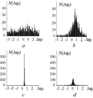
Figure 3: Distribution $N(\Delta\phi_{f})$ of phase difference $\Delta\varphi_{f}$ obtained from series of $10^{3}$ experiments for Rössler systems (8). (a) The asynchronous dynamics takes place ($\varepsilon=0.02$), the distribution of phase shift $\Delta\varphi_{f}$ has been obtained for the spectral components $f\simeq 0.0711$; (b) $\varepsilon=0.02$, $f\simeq 0.1764$; (c) the distribution of phase shift for synchronous spectral component $f\simeq 0.1764$ ($\varepsilon=0.08$) and (d) the analogous distribution for asynchronous spectral component $f\simeq 0.0711$ for the same coupling parameter $\varepsilon=0.08$. Compare with Fig. 1

When the systems demonstrate synchronous behavior the distributions $N(\Delta\phi_{f})$ of phase shift $\Delta\phi_{f}$ are quite different. In this case one can distinguish both synchronized and non-synchronized spectral components characterized by distributions of phase shift of different types. In Fig. 3,c the distribution of $\Delta\phi_{f}$ for synchronous spectral component $\Delta\varphi_{f}$ is shown. One can see that it looks like $\delta$-function that means the phase shift $\Delta\phi_{f}$ is always the same after transient finished. Obviously, this phase shift $\Delta\phi_{f}$ does not depend on initial conditions.

For the non-synchronized spectral components the distributions $N(\Delta\phi_{f})$ are different (see Fig. 3,d). Evidently, in this case the phase shift $\Delta\phi_{f}$ is varied from experiment to experiment. At the same time, the tendency to the synchronization of these spectral components can be observed. The distribution $N(\Delta\phi_{f})$ looks like Gaussian. With the coupling parameter increasing the dispersion of it decreases and the spectral components $f$ of considered Fourier spectra $S_{1,2}(f)$ tend to be synchronized. The same effect can be observed in Fig 1,b-f. With coupling parameter $\varepsilon$ increasing, the points on the $(f,\Delta\phi_{f})$ plane tend to fit a straight line with slope $k=2\pi\tau$ and their scattering decreases.

So, the general criterion of synchronism of identical spectral components $f$ of coupled systems is the establishment of the phase shift (9) after transient finished. It is important to note that the case of classical synchronization of periodical oscillations also obeys to considered criterion (9) (see, e.g., R. Adler (1949)).

Let us consider now the quantitative characteristic of synchronization. In A.E. Hramov, A.A. Koronovskii (2004) the measure of synchronization based on the normalized energy of synchronous time scales has been introduced. The analogous quantity $\rho$ may be defined for Fourier spectra $S(f)$ as

$$\rho_{1,2}=\frac{1}{P}\displaystyle\int\limits_{F_{s}}|S_{1,2}(f)|^{2}\,df\$$ (10)

where $F_{s}$ is the set of synchronized spectral components and

$$P=\displaystyle\int\limits_{0}^{+\infty}|S_{1,2}(f)|^{2}\,df$$ (11)

is the full energy of chaotic oscillations. In fact, the value of $\rho$ is the part of the full system energy corresponding to synchronized Fourier components. This measure $\rho$ is 0 for the nonsynchronized oscillations and 1 for the case of complete and lag synchronization regimes as well as the quantity introduced in A.E. Hramov, A.A. Koronovskii (2004). When the systems undergo transition from asynchronous behavior to the lag synchronization regime the measure of synchronism takes the value between 0 and 1 that corresponds to the case when there are both synchronized and nonsynchronized spectral components in Fourier spectra $S_{1,2}(f)$.

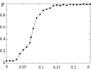
Figure 4: The dependence of the synchronization measure $\rho$ for the first Rössler system (8) on coupling parameter $\varepsilon$

For the real data represented by discrete time series of a finite length one have to use the discrete analog of Fourier transform while the integrals in the relation (10) should be replaced by the sums

$$\rho_{1,2}=\frac{1}{P}\displaystyle\sum\limits_{{j_{s}}}|S_{1,2}(f_{j_{s}})|^{2}\,\Delta f,$$ (12)

where

$$P=\displaystyle\sum\limits_{j}\,|S_{1,2}(f_{j})|^{2}\Delta f.$$ (13)

While the sum in the equation (12) is being calculated only synchronized spectral components $f_{j_{s}}$ should be taken into account.

Figure 4 presents the dependence of the synchronization measure $\rho$ for the first Rössler oscillator of system (8) on the coupling parameter $\varepsilon$. It is clear that the part of the energy corresponding to the synchronized spectral components grows with the coupling strength increasing.

IV Spectral components behavior at the presence of synchronization

Let us now consider how the closed frequency components of two coupled oscillators behave with increase of the coupling strength $\varepsilon$. As a model of such situation let us select two mutually coupled Van-der-Pol oscillators

$$\ddot{x}_{1,2}-\left(\lambda-x^{2}_{1,2}\right)\dot{x}_{1,2}+\Omega_{1,2}^{2}x_{1,2}=\pm\\ \varepsilon(x_{2,1}-x_{1,2}),$$ (14)

where $\Omega_{1,2}=\Omega\pm\Delta$ are slightly mismatched natural cyclic frequencies, $x_{1,2}$ are the variables, describing the behavior of the first and the second self-sustained oscillators, respectively. The parameter $\varepsilon$ characterizes the coupling strength between oscillators. Nonlinearity parameter $\lambda=0.1$ has been chosen small enough in order to make oscillations of self–sustained generators close to the single frequency ones.

Asymmetrical type of coupling in system (14) ensures the appearance of the synchronous regime which is similar to the lag synchronization in chaotic systems. For such type of coupling the oscillations in the synchronous regime are characterized by one frequency $\omega=2\pi f$ while small phase shift $\Delta\varphi_{f}$ between time series $x_{1,2}(t)$, decreasing when coupling strength increases, takes place.

Using the method of complex amplitudes, the solution of equation (14) can be found in the form

$$\begin{split}&x_{1,2}=A_{1,2}e^{i\omega t}+A_{1,2}^{*}e^{-i\omega t},\\ &\dot{A}_{1,2}e^{i\omega t}+\dot{A}^{*}_{1,2}e^{-i\omega t}=0,\end{split}$$ (15)

where “*” means complex conjugation, $\omega$ is the cyclic frequency, at which oscillations in system (14) are realized. One can reduce equations (14) and (15) to the form

$$\dot{A}_{1,2}=\frac{1}{2}\left(\lambda-|A|^{2}\right)A+\\ i\frac{1}{2\omega}\left[\left(\Omega_{1,2}^{2}-\omega^{2}\right)A_{1,2}\mp\varepsilon(A_{2,1}-A_{1,2})\right]$$ (16)

by means of the averaging over the fast changing variables.

Choosing the complex amplitudes in the form of

$$A_{1,2}=r_{1,2}e^{\varphi_{1,2}},$$ (17)

one can obtain the equations for amplitudes $r_{1,2}$ and phases $\varphi_{1,2}$ of coupled oscillators as follows:

$$\begin{split}&\dot{r}_{1,2}=\frac{1}{2}\left(\lambda-|r_{1,2}|^{2}\right)r_{1,2}\pm\frac{\varepsilon r_{2,1}}{2\omega}\sin(\varphi_{1,2}-\varphi_{2,1}),\\ \\ &\displaystyle\dot{\varphi}_{1,2}=\frac{\Omega_{1,2}^{2}-\omega^{2}\pm\varepsilon}{2\omega}\mp\frac{\varepsilon r_{2,1}}{2\omega r_{1,2}}\cos(\varphi_{1,2}-\varphi_{2,1}).\end{split}$$ (18)

The oscillations of two Van-der-Pol generators (14) are synchronized when conditions

$$\dot{r}_{1,2}=0,\qquad\dot{\varphi}_{1,2}=0$$ (19)

are satisfied. Assuming the phase difference of oscillations $\Delta\varphi=\varphi_{2}-\varphi_{1}$ is small enough and taking into account only components of first infinitesimal order over $\Delta\varphi$, one can obtain the relation for the phase shift

$$\Delta\varphi_{1,2}=\frac{\lambda\sqrt{\Omega^{2}+\Delta^{2}\pm 2\sqrt{\Omega\Delta(\varepsilon+\Omega\Delta)}}}{2\varepsilon+4\Omega\Delta}$$ (20)

and frequency

$$\omega_{1,2}=\sqrt{\Omega^{2}+\Delta^{2}\pm 2\sqrt{\Omega\Delta(\varepsilon+\Omega\Delta)}},$$ (21)

which correspond to the stable and nonstable fixed points of the system (18). From relations  (20) and (21) one can see that the phase difference $\Delta\varphi$ of coupled generators is directly proportional to the frequency of oscillations $\omega$ and inversely proportional to the coupling parameter $\varepsilon$ for the small values of detuning parameter $\Delta$

$$\Delta\varphi\simeq\frac{\lambda\omega}{2\varepsilon}.$$ (22)

So, in the synchronous regime the phase shift $\Delta\varphi$ for synchronized frequencies obeys the relation

$$\Delta\varphi\sim{\omega}{\varepsilon^{-1}}.$$ (23)

It is important to note, that the time delay between synchronized spectral components

$$\tau=\frac{\Delta\varphi}{\omega}\sim\varepsilon^{-1}$$ (24)

does not depend upon the frequency, and therefore, the time delays for all frequencies $f$ are equal to each other. Accordingly, the phase shift $\Delta\varphi_{f}$ for the frequency $f$ obeys the relation (5) which is the necessary conditions for lag synchronization appearance. Evidently, if the type of coupling between oscillators is selected in such manner that the phase shift $\Delta\varphi_{f}$ of synchronized spectral components satisfies the condition (23), the appearance of the lag synchronization regime is possible for the large enough values of the coupling strength. Otherwise, if the established phase shift does not satisfy the condition (23), the realization of the lag synchronization regime in the system is not possible for such kind of coupling. So, the relation (23) can be considered as the criterion of the possibility of the existence (or, otherwise, impossibility of existence) of lag synchronization regime in coupled dynamical systems.

The regularity (24) takes place for the large number of dynamical systems and, probably, is universal. Let us consider the manifestations of this regularity for several examples of coupled chaotic dynamical systems.

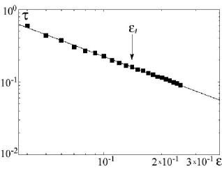
Figure 5: The dependence of time shift $\tau$ between base spectral components ($\blacksquare$ symbols) on coupling parameter $\varepsilon$ for two coupled Rössler systems (8). The straight line corresponds to the power law $\tau\sim\varepsilon^{-1}$. The value of coupling parameter $\varepsilon_{l}\simeq 0.14$ corresponding to the appearance of the lag synchronization regime is shown by the arrow

As the first example we consider the coupled Rössler systems (8) described above. Obviously, one has to consider the phase shift $\Delta\varphi_{f}$ (or time shift $\tau$) of synchronized spectral components to verify the relation (24). As it has been shown above, spectral components characterized by the large value of energy become synchronized first when coupling strength increases. So, the main spectral components $f_{m}$ of Fourier spectra of coupled systems are synchronized in the most lengthy range of the coupled parameter value. Therefore, it is appropriate to consider the time shift $\tau$ of main spectral components for coupling strength values $\varepsilon>0.05$.

In Fig. 5 the dependence of time lag $\tau$ between Fourier-spectra base frequency components of interacting chaotic oscillators on coupling parameter $\varepsilon$ is shown. Base frequency $\omega_{m}=2\pi f_{m}$ of spectrum is close to $\omega=1$ and slightly changes with coupling parameter increasing. In Fig. 5 one can see that after entrainment of Fourier–spectrum base spectral components of interacting oscillators (that corresponds to establishment of time scale synchronization regime, see also A.A. Koronovskii, A.E. Hramov (2004)) the time lag $\tau$, which is between them, obeys the universal power law (24).

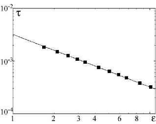
Figure 6: The dependence of time shift $\tau$ between time series $x_{1}(t)$ and $x_{2}(t)$ ($\blacksquare$ symbols) on coupling parameter $\varepsilon$ for two unidirectionally coupled chaotic oscillators (25) and (26). The straight line corresponds to the power law $\tau\sim\varepsilon^{-1}$

As the second example we consider the chaotic synchronization of two unidirectionally coupled Van-der-Pol–Duffing oscillators G.P. King, S.T. Gaito (1992); K. Murali, M. Lakshmanan (1994a); K. Murali, M. Lakshmanan (1994b). The drive generator is described by system of dimensionless differential equations

$$\begin{split}&\dot{x}_{1}=-\nu_{1}\left[x_{1}^{3}-\alpha x_{1}-y_{1}\right],\\ &\dot{y}_{1}=x_{1}-y_{1}-z_{1},\\ &\dot{z}_{1}=\beta y_{1},\end{split}$$ (25)

while the behavior of the response generator is defined by the system

$$\begin{split}&\dot{x}_{2}=-\nu_{2}\left[x_{2}^{3}-\alpha x_{2}-y_{2}\right]+\nu_{2}\varepsilon(x_{1}-x_{2}),\\ &\dot{y}_{2}=x_{2}-y_{2}-z_{2},\\ &\dot{z}_{2}=\beta y_{2},\end{split}$$ (26)

where $x_{1,2}$, $y_{1,2}$ and $z_{1,2}$ are dynamical variables, characterizing states of the drive and response generators, respectively. Values of control parameters are chosen as following: $\alpha=0.35$, $\beta=300$, $\nu_{1}=100$, $\nu_{2}=125$, the difference of parameters $\nu_{1}$ and $\nu_{2}$ provides the slight nonidentity of considered generators.

In Fig. 6 the dependence of time lag $\tau$ between time realizations of coupled oscillators on coupling parameter value $\varepsilon$ is shown. In this range of coupling parameter values the lag synchronization regime is realized. Obviously, the time lag $\tau$ also obeys the power law $\tau\sim\varepsilon^{n}$ with exponent $n=-1$, that corresponds to the relation (24).

V Unstable periodic orbits

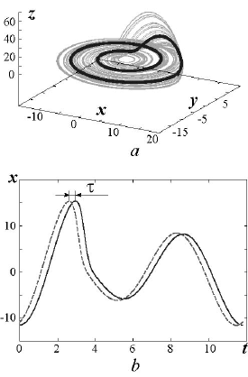
Figure 7: (a) The unstable periodic orbit of the length $m=2$ embedded in the chaotic attractor of the first system. (b) Time series $x_{1}(t)$ and $x_{2}(t)$ corresponding to the “in–phase” unstable saddle orbits of length $m=2$ in the first (solid line) and the second (dashed line) Rössler systems, respectively. The coupling parameter is chosen as $\varepsilon=0.07$. Time shift $\tau$ is denoted by means of the arrow

It is important to note another manifestation of power law (24). It is well known that the unstable periodic orbits (UPOs) embedded into chaotic attractors play the important role in the system dynamics P. Cvitanović (1988); D.P. Lathrop, E.J. Kostelich (1989); P. Cvitanović (1991) including the cases of chaotic synchronization regimes N.F. Rulkov (1996); A. Pikovsky, G. Osipov, M. Rosenblum, M. Zaks, J. Kurths (1997); A. Pikovsky, M. Zaks, M. Rosenblum, G. Osipov, J. Kurths (1997). The synchronization of two coupled chaotic systems in terms of unstable periodic orbits has been discussed in detail in D. Pazó, M. Zaks, J. Kurths (2002). It has been shown that UPOs are also synchronized with each other when the chaotic synchronization in the coupled systems realizes D. Pazó, M. Zaks, J. Kurths (2002). Let us consider the synchronized saddle orbits $m:n$ ($m=n=1,2,\dots$), where $m$ and $n$ are the length of unstable periodic orbits of the first and the second Rössler systems (8), respectively. It was shown that such synchronized orbits may be both “in–phase” and “out–of–phase”, but only “in–phase” orbits exist in all range of coupling parameter values starting from point of the synchronization beginning (see D. Pazó, M. Zaks, J. Kurths (2002) for detail). It is known that the time shift between synchronized “in–phase” orbits decreases with coupling strength increasing. As the UPOs have an influence on the system dynamics (and on the Fourier spectra of the considered systems, too), it seems to be interesting to examine whether the time shift $\tau$ between UPOs obeys the power law (24).

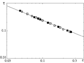
Figure 8: The dependence of time shift $\tau$ between time series $x_{1}(t)$ and $x_{2}(t)$ corresponding to the synchronized saddle orbits of the first and the second Rössler systems on coupling parameter $\varepsilon$. The symbols $\square$ correspond to unstable orbits with length $m=1$, the symbols $\bigcirc$ demonstrate the time shift $\tau$ for the orbits with length $m=2$ and the symbols $\blacksquare$ show this dependence for orbits with length $m=3$. The straight line corresponds to the power law $\tau\sim\varepsilon^{-1}$

To calculate the synchronized saddle orbits we have used the SD–method P. Schmelcher, F.K. Diakonos (1998); D. Pingel, P. Schmelcher, F.K. Diakonos (2001) in the same way as it had been done in D. Pazó, M. Zaks, J. Kurths (2002). The UPO embedded in the chaotic attractor of the first Rössler system and the time series $x_{1,2}(t)$ corresponding to the “in–phase” synchronized UPOs realized in system (8) for coupling strength $\varepsilon=0.07$ is shown in Fig. 7. One can see the presence of the time shift $\tau$ between these time series which can be easily calculated.

The calculated time shift $\tau$ between such “in–phase” synchronized saddle orbits appears to obey the power law $\tau\sim\varepsilon^{-1}$ as well as the spectral components of Fourier spectra do (see Fig. 8). We have examined this relation for “in–phase” UPOs with length $m=1\div 6$ and found the time shift dependence on coupling strength agrees with power law (24) well, but the date is shown in Fig. 8 only for UPOs with length $m=1\div 3$ for the clearness and the simplicity. So, the power law (24) seems to be universal and is manifested in different ways.

VI Conclusion

In conclusion, we have considered the chaotic synchronization of coupled oscillators by means of Fourier spectra; several regularities have been observed.

The chaotic synchronization of coupled oscillators is manifested in the following way. Starting from the certain coupling parameter value the synchronization of the main spectral components of Fourier spectra of interacting chaotic oscillators takes place. Therefore, for these spectral components $f$ the condition (9) is satisfied. In this case one can detect the presence of the time scale synchronization regime (see A.E. Hramov, A.A. Koronovskii (2004); A.E. Hramov, A.A. Koronovskii, P.V. Popov, I.S. Rempen (2005)). If for the considered systems one can introduce correctly the instantaneous phase of chaotic signal V.S. Anishchenko, T.E. Vadivasova (2004); A.E. Hramov, A.A. Koronovskii (2004), one will also detect easily the phase synchronization by means of traditional approach (see, e.g., A. Pikovsky, M. Rosenblum, J. Kurths (2001)).

With further coupling parameter increasing, more spectral components become synchronized. If the coupling between interacting systems is selected in a such way that the lag synchronization regime can be realized then the time shift between synchronized spectral components obeys the power law (24). The spectral components characterized by the large value of energy become synchronized first. Accordingly, the part of energy being fallen on the synchronized spectral components increases from $0$ (asynchronous dynamics) to 1 (the lag synchronization regime). Synchronization of all frequency components corresponds to the appearance of the lag synchronization regime. With further coupling strength increase, the time lag $\tau$ obeying the relation (24) tends to be zero, and related oscillations tend to demonstrate the complete synchronization regime. In this case the time shift $\tau$ between synchronized components does not depend on frequency $f$ of considered components (it is the same for all synchronized components) and obeys the power law (24) with the exponent $n=-1$. The time shift between synchronized “in–phase” UPOs embedded in chaotic attractors also obeys the same power law.

So, in the present paper the mechanism of chaotic synchronization regime appearance in coupled dynamical systems, based on the arising of the phase relation between frequency components of Fourier spectra of interacting chaotic oscillators has been discussed. The obtained results concerning the power law (24) may be also considered as the criterion of possible existence (or, otherwise, impossibility of existence) of lag synchronization regime in coupled dynamical systems (i.e., the lag synchronization regime can not be observed in the coupled chaotic oscillators system unless the time shift between synchronized components obeys the power law  (24)).

References

- A. Pikovsky, M. Rosenblum, J. Kurths (2001) A. Pikovsky., M. Rosenblum, J. Kurths, Synchronization: a universal concept in nonlinear sciences (Cambridge University Press, 2001).
- K. Murali, M. Lakshmanan (1994a) K. Murali, M. Lakshmanan, Phys. Rev. E 48, R1624 (1994a).
- T. Yang T., C.W. Wu and L.O. Chua (1997) T. Yang T., C.W. Wu and L.O. Chua, IEEE Trans. Circuits and Syst. 44, 469 (1997).
- R.C. Elson, A.I. Selverston, R. Huerta, N.F. Rulkov, M.I. Rabinovich, H.D.I. Abarbanel (1998) R.C. Elson, A.I. Selverston, R. Huerta, N.F. Rulkov, M.I. Rabinovich, H.D.I. Abarbanel, Phys. Rev. Lett. 81, 5692 (1998).
- M.D. Prokhorov, V.I. Ponomarenko, V.I. Gridnev, M.B. Bodrov, A.B. Bespyatov (2003) M.D. Prokhorov, V.I. Ponomarenko, V.I. Gridnev, M.B. Bodrov, A.B. Bespyatov, Phys. Rev. E 68, 041913 (2003).
- N.F. Rulkov, M.M. Sushchik, L.S. Tsimring, H.D.I. Abarbanel (1995) N.F. Rulkov, M.M. Sushchik, L.S. Tsimring, H.D.I. Abarbanel, Phys. Rev. E 51, 980 (1995).
- M.G. Rosenblum, A.S. Pikovsky, J. Kurths (1997) M.G. Rosenblum, A.S. Pikovsky, J. Kurths, Phys. Rev. Lett. 78, 4193 (1997).
- L.M. Pecora, T.L. Carroll (1991) L.M. Pecora, T.L. Carroll, Phys. Rev. A 44, 2374 (1991).
- R. Brown, L. Kocarev (2000) R. Brown, L. Kocarev, Chaos 10, 344 (2000).
- S. Boccaletti, J. Kurths, G. Osipov, D.L. Valladares, C.S. Zhou (2002) S. Boccaletti, J. Kurths, G. Osipov, D.L. Valladares, C.S. Zhou, Physics Reports 366, 1 (2002).
- S. Boccaletti., L.M. Pecora, A. Pelaez (2001) S. Boccaletti., L.M. Pecora, A. Pelaez, Phys. Rev. E 63, 066219 (2001).
- A.E. Hramov, A.A. Koronovskii (2004) A.E. Hramov, A.A. Koronovskii, Chaos 14, 603 (2004).
- A.A. Koronovskii, A.E. Hramov (2004) A.A. Koronovskii, A.E. Hramov, JETP Letters 79, 316 (2004).
- B. Torresani (1995) B. Torresani, Continuous wavelet transform (Paris: Savoire, 1995).
- A.A. Koronovskii, A.E. Hramov (2003) A.A. Koronovskii, A.E. Hramov, Continuous wavelet analysis and its applications (In Russian) (Moscow, Fizmatlit, 2003).
- I. Daubechies (1992) I. Daubechies, Ten lectures on wavelets (SIAM, 1992).
- A.E. Hramov, A.A. Koronovskii, P.V. Popov, I.S. Rempen (2005) A.E. Hramov, A.A. Koronovskii, P.V. Popov, I.S. Rempen, Chaos 15, accepted for publication (2005).
- N.F. Rulkov, A.R. Volkovskii, A. Rodriguez-Lozano, E. Del Rio and M.G.Velarde (1994) N.F. Rulkov, A.R. Volkovskii, A. Rodriguez-Lozano, E. Del Rio and M.G.Velarde, Chaos, Solitons & Fractals 4, 201 (1994).
- V.S. Anishchenko, T.E. Vadivasova, D.E. Postnov, M.A. Safonova (1992) V.S. Anishchenko, T.E. Vadivasova, D.E. Postnov, M.A. Safonova, Int. J. Bifurcation and Chaos 2, 633 (1992).
- V.S. Anishchenko, T.E. Vadivasova (2004) V.S. Anishchenko, T.E. Vadivasova, Journal of Communications Technology and Electronics 49, 69 (2004).
- I. Noda, Y. Ozaki (2002) I. Noda, Y. Ozaki, Two–Dimensional Correlation Spectroscopy: Applications in Vibrational and Optical Spectroscopy (John Wiley & Sons, 2002).
- M.G. Rosenblum, A.S. Pikovsky, J. Kurths, G.V. Osipov, I.Z. Kiss, J.L. Hudson (2002) M.G. Rosenblum, A.S. Pikovsky, J. Kurths, G.V. Osipov, I.Z. Kiss, J.L. Hudson, Phys. Rev. Lett. 89, 264102 (2002).
- R. Adler (1949) R. Adler, Proc. IRE. 34, 351 (1949).
- G.P. King, S.T. Gaito (1992) G.P. King, S.T. Gaito, Phys. Rev. A 46, 3092 (1992).
- K. Murali, M. Lakshmanan (1994b) K. Murali, M. Lakshmanan, Phys. Rev. E 49, 4882 (1994b).
- P. Cvitanović (1988) P. Cvitanović, Phys. Rev. Lett. 61, 2729 (1988).
- D.P. Lathrop, E.J. Kostelich (1989) D.P. Lathrop, E.J. Kostelich, Phys. Rev. A 40, 4028 (1989).
- P. Cvitanović (1991) P. Cvitanović, Physica D 51 (1991).
- N.F. Rulkov (1996) N.F. Rulkov, Chaos 6, 262 (1996).
- A. Pikovsky, G. Osipov, M. Rosenblum, M. Zaks, J. Kurths (1997) A. Pikovsky, G. Osipov, M. Rosenblum, M. Zaks, J. Kurths, Phys. Rev. Lett. 79, 47 (1997).
- A. Pikovsky, M. Zaks, M. Rosenblum, G. Osipov, J. Kurths (1997) A. Pikovsky, M. Zaks, M. Rosenblum, G. Osipov, J. Kurths, Chaos 7, 680 (1997).
- D. Pazó, M. Zaks, J. Kurths (2002) D. Pazó, M. Zaks, J. Kurths, Chaos 13, 309 (2002).
- P. Schmelcher, F.K. Diakonos (1998) P. Schmelcher, F.K. Diakonos, Phys. Rev. E 57, 2739 (1998).
- D. Pingel, P. Schmelcher, F.K. Diakonos (2001) D. Pingel, P. Schmelcher, F.K. Diakonos, Phys. Rev. E 64, 026214 (2001).