On Deviations from Gaussian Statistics for Surface Gravity Waves

Abstract

Here we discuss some issues concerning the statistical properties of ocean surface waves. We show that, using the approach of weak turbulence theory, deviations from Gaussian statistics can be naturally included. In particular we discuss the role of bound and free modes for the determination of the statistical properties of the surface elevation. General formulas for skewness and kurtosis as a function of the spectral wave action density are here derived.

I Introduction

Recently it has been observed experimentally that large amplitude waves can appear on the surface of the ocean. There are different mechanisms that can lead to the formation of such events. For example, linear theory can be considered as a first candidate for explaining these waves: it can happen that for some fortuitous occasion, two or more waves of different lengths are in phase, leading to the well known constructive interference mechanism (linear superposition of Fourier modes). When the surface elevation is characterized by a large number of linear waves with random phases, it is possible to estimate the probability of measuring an extreme event (say a wave of height larger than 2 times the significant wave height). This theoretical task has been accomplished about 50 years ago LH52 and the main result is that, if the surface elevation is Gaussian and the process is narrow-banded, then wave heights and wave crests are distributed according to the Rayleigh distribution (corrections due to finite spectral band-width have also been obtained).

First substantial corrections to this distribution can be obtained if waves are considered weakly nonlinear, or more precisely, if for each wave component (free modes), its bound contributions are included. For the narrow-banded case this is nothing but describing the surface elevation as a Stokes expansion. The more general description of the surface elevation, valid for any spectral band-width, was given in a seminal paper by Longuet-Higgins LH63 . He was able to derive the contributions to the surface elvation from bound waves up to second order in wave steepness. The numerical implementation of the formulas reported in the paper by Longuet-Higgins corresponds to what today is called a “second order theory” (see FOR00 ); note that the theory includes only bound modes and not free modes. The presence of those Stokes-like contributions gives the waves the well known property of being positively skewed. Using the second order theory, TAY80 was able to include this contribution in the distribution function of the wave crests. More in particular, for unidirectional narrow-banded waves in infinite water depth, with the hypothesis that free waves are described by a Gaussian statistics, he derived a formula for the distribution of wave crests (now known as the Tayfun distribution) which does bring substantial corrections to the Rayleigh distribution, especially if the wave steepness is large. It should be here stressed that the Tayfun second order theory predicts a Rayleigh distribution for wave heights (this is because second order contributions cancel out for wave heights). The Tayfun distribution has been recently compared successfully with interesting numerical experiments of envelope equations (see SO05 ). Paradoxically, the distribution describes very well the data characterized by large directional spreading but underestimates wave crests in the long-crested case for which the distribution has been derived.

Only in the last few years it was realized that not only bound modes can generate deviations from a Gaussian statistics but also the dynamics of free waves should be considered in the determination of the statistical properties of the surface elevation. More in particular, it was shown in ONO01 and JAN03 that the nonlinear interactions of free modes can substantially alter the statistical properties of the surface elevation. Note that in this case the statistics of free mode (without the contribution from bound modes) can be non Gaussian. It was also found that the nonlinear interactions responsible for such a deviation from gaussian statistics are associated with the modulational instability mechanism (also known as the Benjami-Feir instability) which can be thought as a quasi-resonant 4 wave interaction. Those concepts are the bases of the theory developed in JAN03 , where a kinetic equation that includes quasi-resonant interactions is derived. More than that, in the same paper, an equation that relates the kurtosis (fourth moment of the surface elevation) to the spectral wave action density is obtained. The theory includes only the contribution to the kurtosis from free modes.

The aim of the present paper is to describe a single theory, based on the Hamiltonian formulation of surface gravity waves, that can take into account both the contribution of bound and free waves. Before entering in the discussion we will motivate the importance of including the free wave dynamics in the theory by showing some experimental data recorded during the Marintek experiments ONO04 . Here we anticipate that the experimental data suggest that in the particular condition of long crested waves and large Benjamin-Feir Index, the second order theory is inadequate to describe the distribution of wave crests. In the last part of the paper we will sketch the derivation of the formulas for the kurtosis and skewness which include both the contribution from bound and free modes.

II Data from Marintek compared with the Second Order Theory

Here we will consider some experimental data recorded at Marintek in one of the largest wave tank in the world. The length of the tank is $270$ $m$ and its width is $10.5$ $m$. The conditions at the wave maker were provided by a Jonswap spectrum with random phases. One accepts this fact and then lets the phases (and amplitudes) evolve according to the nonlinear dynamics. Different runs were performed (see ONO04 ). Here we will consider just the probability density function of wave crests for the run characterized by a strong nonlinearity (steepness calculated as $\epsilon=H_{s}k_{p}/2$ was about 0.15, with $H_{s}$ the significant wave height and $k_{p}$ the wave-number of the peak of the spectrum, computed using the linear dispersion relation from the peak frequency). Experimental data are compared with numerical data from a standard second order theory (the coupling coefficient has been taken from FOR00 and with the Tayfun distribution.

In figure  1 we show a comparison between experimental the wave crest distribution recorded at the first probe, a few wave lengths from the wave maker, and the second order theory. First of all, it should be mentioned that for the present conditions the Tayfun theory is in good agreement with second order theory; the experimental data are not so far from the mentioned distributions.

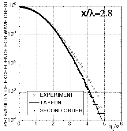
Figure 1: Wave crest distribution: experimental data, measured at 2.8 wavelengths from the wave maker, are compared with data from Tayfun and second order theory.

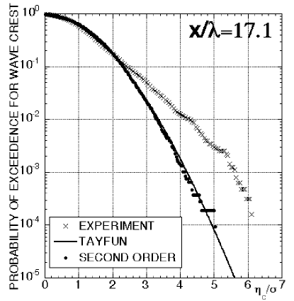
Figure 2: Wave crest distribution: experimental data, recorded at 17.1 wavelengths from the wave maker, are compared with data from Tayfun and second order theory.

This is not a surprise because data have been built as a linear superposition of Fourier modes and the generation of bound modes is practically instantaneous with respect to the Benjamin-Feir space scales. The situation is different after the waves have evolved along the tank according to their nonlinear dynamics. As can be seen in figure  2, the Tayfun distribution (and the second order theory) completely underestimate the experimental data. This result is quite significant because it clearly tells us that there are some statistically stationary conditions in which the second order theory is completely inadequate to describe the probability density function of real water waves.

Apparently there is no reason for the second order theory to fail to reproduce the experimental data; data (steepness and spectral shape considered) do not violate any of the assumption for deriving the second order theory. In the second order theory the surface elevation is considered as a linear superposition of non interacting free modes to which bound modes have been added. The main problem in the approach is that, as it is well known from Hasselmann-Zakharov theory (HAS62 , ZAK67 ), free waves also interact. In the next section we will consider a general theory which considers both the contribution from bound modes and free modes.

III Skewness and Kurtosis: Contribution from Bound and Free Waves

The goal of this section is to derive formulas for the skewness and the kurtosis as a function of the spectral wave action density. The starting point for the derivation of the theory is the Hamiltonian description of surface gravity waves (see ZAK68 and ZAK99 ). The theory described below is general and can be applied to any weakly nonlinear dispersive system. Here we will start with the following Hamiltonian, truncated to four-wave interactions:

$$\begin{split}&H=\int\omega_{0}a_{0}a_{0}^{*}dk_{0}+\\ &+\int U^{(1)}_{0,1,2}(a_{0}a_{1}^{*}a_{2}^{*}+a_{0}^{*}a_{1}a_{2})\delta_{0-1-2}dk_{012}+\\ &+\frac{1}{3}\int U^{(2)}_{0,1,2}(a_{0}^{*}a_{1}^{*}a_{2}^{*}+a_{0}a_{1}a_{2})\delta_{0+1+2}dk_{012}+\\ &+\frac{1}{2}\int V^{(2)}_{0,1,2,3}a_{0}^{*}a_{1}^{*}a_{2}a_{3}\delta_{0+1-2-3}dk_{0123}+...\end{split}$$ (1)

The notation is taken from KRA94 (for example, $a_{i}=a({\bf k}_{i})$, $U^{(1)}_{0,1,2}=U^{(1)}({\bf k}_{0},{\bf k}_{1},{\bf k}_{2})$). The coupling coefficients and their properties are reported in the just mentioned paper (the reader unfamiliar with the present Hamiltonian description of surface gravity waves who is willing to understand details of what follows is strongly advised to read the paper KRA94 ). Note that we have for brevity omitted three more integrals which contain non resonant four-wave interactions. Up to our desired accuracy, those terms do not contribute to the skewness and to the kurtosis, therefore can be safely neglected. The surface elevation $\eta({\bf k})$ and the velocity potential $\psi({\bf k})$ are related to the wave action variable $a({\bf k})$ in the following way (note that the dependence on time has been omitted for brevity):

$$\eta({\bf k})=\sqrt{\frac{k}{2\omega({\bf k})}}(a({\bf k})+a^{*}(-{\bf k}))$$ (2)

$$\psi({\bf k})=-i\sqrt{\frac{\omega({\bf k})}{2k}}(a({\bf k})-a^{*}(-{\bf k})).$$ (3)

It is well known that three waves resonant interactions are forbidden for surface gravity waves, therefore it is always possible to introduce new canonical variables $b$ and $b^{*}$ for which the Hamiltonian does not show explicitly those interactions. The standard way of doing this consists in considering the canonical transformation, expressed as the following infinite series:

$$\begin{split}a_{0}=b_{0}+&\int A^{(1)}_{0,1,2}b_{1}b_{2}\delta_{0-1-2}dk_{12}+\\ &+\int A^{(2)}_{0,1,2}b_{1}^{*}b_{2}\delta_{0+1-2}dk_{12}+\\ &+\int A^{(3}_{0,1,2}b_{1}^{*}b_{2}^{*}\delta_{0+1+2}dk_{12}+...\end{split}$$ (4)

The canonical transformation allows one to separate directly the bound modes from the free modes: modes $b(\bf k)$ are free modes which have their own dynamics and the surface elevation (which contains free and bound modes) can be recovered directly by using equations (2) and (4). Indeed, it is easy to show that in the narrow-banded approximation equations (2) and (4) reduce to the Stokes expansion, i.e. a carrier wave plus its bound harmonics.

Before entering into the details, here we mention that we will make large use of the so called quasi-gaussian approximation, i.e. the goal is to express the higher order correlators as a function of the second order correlator, $<b_{1}b_{2}^{*}>=N_{1}\delta_{1-2}$, with $N=N({\bf k})$ the wave action density spectrum ($<...>$ indicate ensemble averages). In this approximation the fourth and six order correlators for the free waves can be writen as follows (see for example JAN03 )

$$<b_{1}b_{2}b_{3}^{*}b_{4}^{*}>=N_{1}N_{2}(\delta_{1-3}\delta_{2-4}+\delta_{1-4}\delta_{2-3})+D_{1,2,3,4}$$ (5)

$$\begin{split}<b_{1}b_{2}b_{3}b_{3}^{*}b_{4}^{*}b_{5}^{*}>&=N_{1}N_{2}N3\\ &(\delta_{1-4}\delta_{2-5}\delta_{3-6}+\delta_{1-4}\delta_{2-6}\delta_{3-5}+\\ &+\delta_{1-5}\delta_{2-4}\delta_{3-6}+\delta_{1-5}\delta_{2-6}\delta_{3-4}+\\ &+\delta_{1-6}\delta_{2-4}\delta_{3-5}+\delta_{1-6}\delta_{2-5}\delta_{3-4})\end{split}$$ (6)

$D_{1,2,3,4}$ is the cumulant, irreducible part of the fourth order correlator (for the sixth order correlator it has been neglected). Note that, for a gaussian process $D_{1,2,3,4}$ is exactly zero. Therefore, in order to describe departures from gaussian behavior we consider an evolution equation for $D_{1,2,3,4}$. This can be accomplished starting with the evolution equation for the free waves (the Zakharov equation) and developing evolution equations for the second and fourth moment of $a({\bf k})$. the equation for $D_{1,2,3,4}$ can be solved supposing that the wave action density spectrum changes on a slow time scale and that at time $t=0$ the waves are Gaussian (the cumulant is exactly zero). Details can be found in JAN03 . The result is the following equation for $D_{1,2,3,4}$:

$$\begin{split}D_{1,2,3,4}=&2T_{1,2,3,4}\delta_{1+2-3-4}G(\Delta\omega,t)\\ &N_{1}N_{2}(N_{3}+N_{4})-(N_{1}+N_{2})N_{3}N_{4}\end{split}$$ (7)

$T_{1,2,3,4}$ is the coupling coefficient for the Zakharov equation and $G(\Delta\omega,t)$ is given by:

$$G(\Delta\omega,t)=\frac{1-Cos(\Delta\omega t)}{\Delta\omega}+i\frac{Sin(\Delta\omega t)}{\Delta\omega}$$ (8)

with $\Delta\omega=\omega_{1}+\omega_{2}-\omega_{3}-\omega_{4}$. We now consider the statistical properties of the weakly nonlinear system described by the Hamiltonian in (1). We consider the third order moment $<\eta({\bf x})^{3}>$; using the definition of the Fourier transform and equation (2) we obtain:

$$\begin{split}&<\eta({\bf x})^{3}>=\int L_{1,2,3}(<a_{1}a_{2}a_{3}>+\\ &+<a_{1}^{*}a_{2}^{*}a_{3}^{*}>)\delta_{123}dk_{123}+3\int L_{1,2,3}(<a_{1}a_{2}a_{3}^{*}>+\\ &+<a_{1}^{*}a_{2}^{*}a_{3}>)\delta_{1+2-3}dk_{123}\end{split}$$ (9)

where

$$L_{1,2,3}=\sqrt{\frac{\omega_{1}\omega_{2}\omega_{3}}{8g^{3}}}$$ (10)

Note that $L_{1,2,3}$ is symmetric under the transposition of all subscripts. We now use the canonical transformation (4) and insert it in (9) to obtain:

$$\begin{split}<\eta({\bf x})^{3}>=&\int S_{1,2,3,4}(<b_{1}b_{2}b_{3}^{*}b_{4}^{*}>+\\ &<b_{1}^{*}b_{2}^{*}b_{3}b_{4}>)\delta_{1+2-3-4}dk_{1234}\end{split}$$ (11)

where the kernel $S_{1,2,3,4}$ is given in ONO05 where also intermediate steps in the derivation are reported. Here we just mention that $S_{1,2,3,4}$ is a function of $A^{(1)}$, $A^{(2)}$ and $A^{(3)}$ in the canonical trnasformation. Now using equations (5) and (7) we can write the skewness as:

$$\begin{split}&<\eta({\bf x})^{3}>=4\int S_{1,2,1,2}N_{1}N_{2}dk_{12}+\\ &+16\int S_{1,2,3,4}T_{1,2,3,4}N_{1}N_{2}N_{3}\frac{1-Cos(\Delta\omega t)}{\Delta\omega}\\ &\delta_{1+2-3-4}dk_{1234}\end{split}$$ (12)

The final result is that the skewness can be written as the sum of two contributions: the first one includes only bound modes and the second one depends both on bound and free modes.

We now consider the kurtosis. Using a similar approach used to derive equation (12), we write the kurtosis in the following way:

$$\begin{split}<\eta({\bf x})^{4}>=&\int M_{1,2,3,4}(<a_{1}a_{2}a^{*}_{3}a^{*}_{4}>+\\ &+<a_{1}^{*}a_{2}^{*}a_{3}a_{4}>)\delta_{1+2-3-4}dk_{1234}\end{split}$$ (13)

where

$$M_{1,2,3,4}=\frac{3}{4g^{2}}\sqrt{\omega_{1}\omega_{2}\omega_{3}\omega_{4}}$$ (14)

Using the canonical transformation, we obtain

$$\begin{split}&<\eta({\bf x})^{4}>=\int M_{1,2,3,4}(<b_{1}b_{2}b^{*}_{3}b^{*}_{4}>+\\ &+<b_{1}b_{2}b^{*}_{3}b^{*}_{4}>)\delta_{1+2-3-4}dk_{1234}+\\ &\int K_{1,2,3,4,5,6}(<b_{1}b_{2}b_{3}b_{4}^{*}b_{5}^{*}b_{6}^{*}>+\\ &<b_{1}b_{2}b_{3}b_{4}^{*}b_{5}^{*}b_{6}^{*}>)\delta_{1+2+3-4-5-6}dk_{123456}\end{split}$$ (15)

The kernel $K_{1,2,3,4,5,6}$, given in ONO05 , is a function of $A^{(1)}$, $A^{(2)}$, $A^{(3)}$. Note that at the same order, higher order terms that we have omitted in the canonical transformation should enter (those terms are reported in ONO05 ). We now apply the quasi- gaussian approximation and use equations (5) and (6) for the fourth and sixth order correlator to obtain:

$$\begin{split}&<\eta({\bf x})^{4}>=3<\eta({\bf x})^{2}>^{2}+\\ &+16\int M_{1,2,3,4}T_{1,2,3,4}N_{1}N_{2}N_{3}\frac{1-Cos(\Delta\omega t)}{\Delta\omega}\\ &\delta_{1+2-3-4}dk_{1234}+12\int K_{1,2,3,1,2,3}N_{1}N_{2}N_{3}dk_{123}\end{split}$$ (16)

This is the final formula for the kurtosis expressed as a sum of 3 contributions: the first one corresponds to a pure gaussian system, the second one is the contribution from free modes and the last one is the contribution from bound modes. Equations (12) and (16) are valid for long and short crested waves. It is interesting to note that in the limit of long-crested waves and in the narrow-banded approximation the integral including free modes becomes proportional to the Benjamin-Feir Index (see JAN03 for details), while the integral including bound modes become proportional to the steepness squared.

As a conclusion we may state that the main contribution of the paper is the derivation of equations (12) and (16). Those equations, obtained using the Hamiltonian formulation of surface gravity waves, can be viewed as a generalization and unification of the theory developed by Longuet-Higgins in 1963 on bound modes and the theory developed by Janssen in 2003 on free modes.

Acknowledgments The experimental work at Marintek (Norway) has been supported by the Improving Human Potential - Transnational Access to Research Infrastructures Programme of the European Commission under the contract HPRI-CT-2001-00176. This research has also been supported by the U.S. Army Engineer Research and Development Center. MIUR is also acknowledged.

References

- (1) Forristall, G.Z. Wave Crest Distributions: Observations and Second-Order Theory Journal of Phys. Ocean., 30, 1931-1943, 2000.
- (2) Hasselmann, K., On the non-linear energy transfer in a gravity wave spectrum, part 1: general theory, Journal of Fluid Mechanics, 12, 481-501, 1962.
- (3) Jannsen, P.A.E.M., Nonlinear Four-Wave Interactions and Freak Waves, J. Physical Ocean. 33, 863 883, 2003.
- (4) Krasitskii, V.P., On reduced equations in the Hamiltonian theory of weakly nonlinear surface waves, J. Fluid Mech. 272, 1, 1994.
- (5) Longuet-Higgins, M. S., On the statistical distribution of the heights of sea waves, J. Marine Res. 11, 1245–1266, 1952.
- (6) Longuet-Higgins, M. S., The effect of non-linearities on statistical distributions in the theory of sea waves, J. Fluid. Mech. 17, 459–480, 1963.
- (7) Onorato, M., Osborne, A.R., Serio, Bertone, S., Freak waves in random oceanic sea states, Phys. Rev. Letters, 86, 5831 - 5834, 2001.
- (8) Onorato, M., Osborne, A.R., Serio, Cavaleri, L., Brandini, C., and Stansberg, C.T., Observation of strongly non-Gaussian statistics for random sea surface gravity waves in wave flume experiments Phys. Rev E 70 (6): Art. No. 067302, 2004. See also Onorato, M., Osborne, A.R., Serio, Cavaleri, L., Brandini, C., Stansberg, C.T., Extreme waves and modulational instability: wave flume experiments on irregular waves. submitted for pubblication, 2004.
- (9) Onorato, M., On the statistical properties of surface gravity waves, in preparation, 2005
- (10) Socquet-Juglard, H., Dysthge, K., Trulsen, K., Krogstad, H.E., Liu J., Distribution of surface gravity waves during spectral changes, submitted to Journal Fluid Mech., 2005.
- (11) Tayfun, M. A., Narrow-band nonlinear sea waves J. Geophys. Res., 85, 1548–1552, 1980.
- (12) Zakharov, V. E. and Filonenko N. N., Energy spectrum for stochastic oscillations of the surface of a liquid, Soviet Phys. Dokl.,11, 881-883, 1967.
- (13) Zakharov, V.E. Stability of periodic waves of finithe amplitude on the surface of a deep liquid, J. Appl. Mech. Tech. Phys., 2, 190-194, 1968.
- (14) Zakharov, V.E. Statistical theory of gravity and capillary waves on the surface of a finite-depth fluid, Eur. J. Mech. B/Fluids, 18, 327-344, 1999.