Effective dynamics in Hamiltonian systems with mixed phase space

Abstract

An adequate characterization of the dynamics of Hamiltonian systems at physically relevant scales has been largely lacking. Here we investigate this fundamental problem and we show that the finite-scale Hamiltonian dynamics is governed by effective dynamical invariants, which are significantly different from the dynamical invariants that describe the asymptotic Hamiltonian dynamics. The effective invariants depend both on the scale of resolution and the region of the phase space under consideration, and they are naturally interpreted within a framework in which the nonhyperbolic dynamics of the Hamiltonian system is modeled as a chain of hyperbolic systems.

I Introduction

A comprehensive understanding of Hamiltonian dynamics is a long outstanding problem in nonlinear and statistical physics, which has important applications in various other areas of physics. Typical Hamiltonian systems are nonhyperbolic as they exhibit mixed phase space with coexisting regular and chaotic regions. Over the past years, a number of ground-breaking works chirikov1 ; asymp ; meiss1 ; greene1 ; pikovsky1 ; christiansen1 ; lau1 ; zasl ; uptodate have increasingly elucidated the asymptotic behavior of such systems and it is now well understood that, because of the stickiness due to Kolmogorov-Arnold-Moser (KAM) tori, the chaotic dynamics of typical Hamiltonian systems is fundamentally different from that of hyperbolic, fully chaotic systems. Here “asymptotic” means in the limit of large time scales and small length scales. But in realistic situations, the time and length scales are limited. In the case of hyperbolic systems, this is not a constraint because the (statistical) self-similarity of the underlying invariant sets guarantees the fast convergence of the dynamical invariants (entropies, Lyapunov exponents, fractal dimensions, escape rates, etc) and the asymptotic dynamics turns out to be a very good approximation of the dynamics at finite scales. In nonhyperbolic systems, however, the self-similarity is usually lost because the invariant sets are not statistically invariant under magnifications. As a result, the finite-scale behavior of a Hamiltonian system may be fundamentally different from the asymptotic behavior considered previously, which is in turn hard to come by either numerically uptodate ; fluid or experimentally nh_h .

The aim of this paper is to study the dynamics of Hamiltonian systems at finite, physically relevant scales. To the best of our knowledge, this problem has not been considered before. Herewith we focus on Hamiltonian chaotic scattering, which is one of the most prevalent manifestations of chaos in open systems, with examples ranging from fluid dynamics fluid ; nh_h to solid-state physics sol_stat to general relativity relat . We show that the finite-scale dynamics of a Hamiltonian system is characterized by effective dynamical invariants (e.g., effective fractal dimension), which: (1) may be significantly different from the corresponding invariants of the asymptotic dynamics; (2) depend on the resolution but can be regarded as constants over many decades in a given region of the phase space; and (3) may change drastically from one region to another of the same dynamically connected (ergodic) component. These features are associated with the slow and nonuniform convergence of the invariant measure due to the breakdown of self-similarity in nonhyperbolic systems. To illustrate the mechanism behind the properties of the effective invariants, we introduce a simple deterministic model which we build on the observation that a Hamiltonian system can be represented as a chain of hyperbolic systems.

The paper is organized as follows. We start, in Sec. II, with the analysis of the invariant measure and the outline of the transport structures underlying its convergence. Our chain model is introduced and analyzed in Sec. III. The effective fractal dimension is defined in Sec. IV and its properties are verified for a specific system in Sec. V. Conclusions are presented in the last section.

II Invariant Measure

For concreteness, consider a two-dimensional area preserving map with a major KAM island surrounded by a chaotic region. One such map captures all the main properties of a wide class of Hamiltonian systems with mixed phase space. When the system is open (scattering), almost all particles initialized in the chaotic region eventually escape to infinity. We first study this case with a diffusive model for the transversal motion close to the main KAM island, obtaining an analytical expression for the probability density $\rho(x,t)$ of particles remaining in the scattering region at time $t$ and distance $x$ from the island [see APPENDIX]. We find that, in the case of chaotic scattering, a singularity develops and the invariant measure, given by $\lim_{t\rightarrow\infty}\rho(x,t)$, accumulates on the outermost KAM torus of the KAM island [APPENDIX]. Physically, this corresponds to the tendency of nonescaping particles to concentrate around the regular regions. Dynamically, the stickiness due to KAM tori underlies two major features of Hamiltonian chaotic scattering, namely the algebraic decay of the survival probability of particles in the scattering region asymp ; meiss1 ; greene1 ; pikovsky1 ; christiansen1 and the integer dimension of the chaotic saddle lau1 , and distinguishes this phenomenon from the hyperbolic chaotic scattering characterized by exponential decay and noninteger fractal dimension. However, the convergence of the measure is rather slow and highly nonuniform, as shown in Fig. 1 for typical parameters, which is in sharp contrast with the fast, uniform convergence observed in hyperbolic systems. Our main results are ultimately related to this slow and nonuniform convergence of the invariant measure.

Previous works on transport in Hamiltonian systems have used stochastic models, where invariant structures around KAM islands are smoothened out and the dynamics is given entirely in terms of a diffusion equation chirikov1 ; greene1 or a set of transition probabilities (Markov chains or trees) meiss1 ; other_chains . The stochastic approach is suitable to describe transport properties (as above), but cannot be used to predict the behavior of dynamical invariants such as Lyapunov exponents and fractal dimensions. Here we adopt a deterministic approach where we use the Cantori surrounding the KAM islands to split the nonhyperbolic dynamics of the Hamiltonian system into a chain of hyperbolic dynamical systems.

Cantori are invariant structures that determine the transversal transport close to the KAM islands asymp ; meiss1 . There is a hierarchy of infinitely many Cantori around each island. Let $C_{1}$ denote the area of the scattering region outside the outermost Cantorus, $C_{2}$ denote the annular area in between the first and second Cantorus, and so on. As $j$ is increased, $C_{j}$ becomes thinner and approaches the corresponding island. For simplicity, we consider that there is a single island hier and that, in each iteration, a particle in $C_{j}$ may either move to the outer level $C_{j-1}$ or the inner level $C_{j+1}$ or stay in the same level meiss1 . Let $\Delta_{j}^{-}$ and $\Delta_{j}^{+}$ denote the transition probabilities from level $j$ to $j-1$ and $j+1$, respectively. A particle in $C_{1}$ may also leave the scattering region, and in this case we consider that the particle has escaped. The escaping region is denoted by $C_{0}$. The chaotic saddle is expected to have points in $C_{j}$ for all $j\geq 1$. It is natural to assume that the transition probabilities $\Delta_{j}^{-}$ and $\Delta_{j}^{+}$ are constant in time. This means that each individual level can be regarded as a hyperbolic scattering system, with its characteristic exponential decay and noninteger chaotic saddle dimension. Therefore, a nonhyperbolic scattering is in many respects similar to a sequence of hyperbolic scatterings.

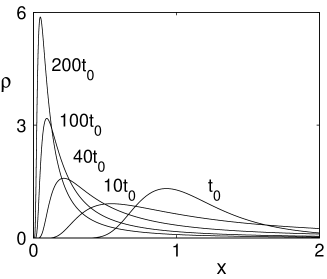
Figure 1: Snapshots of the probability density $\rho$ as a function of $x$, for $\rho(x,0)=\delta(x-x_{0})$, $x_{0}=1$, $x_{1}=2$, $\alpha=3$, and the outermost torus of the KAM island at $x=0$ [APPENDIX]. The time $t$ is indicated in the figure.

III Chain Model

We now introduce a simple deterministic model that incorporates the above elements and reproduces essential features of the Hamiltonian dynamics. Our model is depicted in Fig. 2 and consists of a semi-infinite chain of 1-dimensional “$/\backslash/$-shaped” maps, defined as follows:

$$M_{j}(x)=\left\{\begin{array}[]{lll}&\xi_{j}x,&0\leq x<1/\xi_{j}\\ -&\xi_{j}(x-\Delta_{j}^{-})+2,&1/\xi_{j}<x-\Delta_{j}^{-}<2/\xi_{j}\\ &\xi_{j}(x-1)+1,&-1/\xi_{j}<x-1\leq 0,\end{array}\right.$$

where $\xi_{j}>3$ and $0<\Delta_{j}^{-}<1-3/\xi_{j}\;$ ($j=1,2,\ldots$). If $x$ falls in the interval $1/\xi_{j}\leq x\leq 1/\xi_{j}+\Delta_{j}^{-}$, where $M_{j}$ is not defined, the “particle” is considered to have crossed a Cantorus to the “outer level” $j-1$. This interval is mapped uniformly to $[0,1]$, and the iteration proceeds through $M_{j-1}$. Symbolically, this is indicated by $j\rightarrow j-1$. Similarly, if $x$ falls into $1-1/\xi_{j}-\Delta_{j}^{+}\leq x\leq 1-1/\xi_{j}$, where $\Delta_{j}^{+}=1-3/\xi_{j}-\Delta_{j}^{-}$, the particle goes to the “inner level”, and $j\rightarrow j+1$. Particles that reach $1/\xi_{1}\leq x\leq 1/\xi_{1}+\Delta_{1}^{-}$ are considered to have escaped. The domain of $M_{j}$ is denoted by $I_{j}$ and is analogous to $C_{j}$ in a Hamiltonian system, where $\Delta_{j}^{-}$ and $\Delta_{j}^{+}$ represent the transition probabilities. The transition rate ratios $\mu=\Delta_{j}^{+}/\Delta_{j}^{-}$ and $\nu=\Delta_{j+1}/\Delta_{j}$ are taken in the interval $0<\mu<\nu<1$ and are set to be independent of $j$, where $\Delta_{j}=\Delta_{j}^{+}+\Delta_{j}^{-}$. The parameter $\mu$ is a measure of the fraction of particles in a level $j$ that will move to the inner level $j+1$ when leaving level $j$, while $\nu$ is a measure of how much longer it takes for the particles in the inner level to escape. The nondependence on $j$ corresponds to the approximate scaling of the Cantori suggested by the renormalization theory meiss1 . Despite the hyperbolicity of each map, the entire chain behaves as a nonhyperbolic system. For a uniform initial distribution in $I_{1}$, it is not difficult to show details that the number of particles remaining in the chain after a long time $t$ decays algebraically as $Q(t)\sim t^{-\ln\mu/\ln\nu}$, and that the initial conditions of never escaping particles form a zero Lebesgue measure fractal set with box-counting dimension 1. However, the finite-scale behavior may deviate considerably from these asymptotics, as shown in Fig. 3.

Figure 2: Semi-infinite chain of hyperbolic maps $M_{j}$, $j=1,2,\ldots$

In Fig. 3(a) we show the survival probability $Q$ as a function of time. For small $\mu$ and $\nu$, the curve is composed of a discrete sequence of exponentials with scaling exponents $\ln(1-\Delta_{j}^{-})$, which decrease (in absolute value) as we go forward in the sequence. The length of each exponential segment is of the order of $\mu$ in the decay of $Q$ and $-\ln\nu$ in the variation of $\ln t$. This striking behavior is related to the time evolution of the density of particles inside the chain. This is shown in Fig. 3(b), where we plot the average position $\langle j\rangle$ of an ensemble of particles initialized in $I_{1}$ (i.e., $j=1$). The transitions between successive exponentials in the decay of $Q$ [Fig. 3(a)] match the transitions from a level $j$ to the next in the average position of the remaining particles [Fig. 3(b)]. In a Hamiltonian system, the increase of $\langle j\rangle$ in time is related to the development of the singular invariant measure anticipated in our diffusion analysis [see Fig. 1]. The piecewise exponential behavior of $Q$ is smoothened out for large $\mu$ and $\nu>\mu$ [Figs. 3(a) and 3(b)].

In Fig. 3(c) we show the fractal dimension of the set of initial conditions of never escaping particles as computed from the uncertainty algorithm uncert , which consists in measuring the scaling of the fraction $f(\varepsilon)$ of $\varepsilon$-uncertain points (initial points whose escaping time is different from the escaping time of points taken $\varepsilon$ apart). The scaling is statistically well defined over decades and the exponent $\alpha=\Delta\ln f(\varepsilon)/\Delta\ln\varepsilon$ can be computed accurately. However, the resulting dimension $1-\alpha$ is not only significantly smaller than 1 but also depends critically on the region $L$ of the phase space where it is computed. The convergence of the dimension is indeed so slow that it can only be noticed when observed over very many decades of resolution, as shown in Fig. 3(d) where data of Fig. 3(c) is plotted over 35 decades! Initially smaller, the dimension measured for $L=I_{1}$ approaches the dimension measured for $L=I_{2}$ as the scale $\varepsilon$ is reduced beyond $10^{-15}$ (i.e. the corresponding curves in Fig. 3(d) become parallel). As shown in Fig. 3(d), this behavior is related to a transition in the average innermost level $\langle j_{max}\rangle$ reached by the particles launched from $\varepsilon$-uncertain points. As $\varepsilon$ is further reduced, new transitions are expected. The dimension measured in between transitions is mainly determined by the dimension $D=\ln 3/\ln\xi_{k}$, $k=\langle j_{max}\rangle$, of the corresponding element of the chain. For given $j$ and $\varepsilon$, the measured dimension is larger when $L$ is taken in a denser part of the invariant set, such as in the subinterval of $I_{1}$ first mapped into $I_{2}$ [Fig. 3(c); diamonds], because $\langle j_{max}\rangle$ is larger in these regions. In some regions, however, the measured dimension is quite different from the asymptotic value even at scales as small as $\varepsilon=10^{-30}$. This slow convergence of the dimension is due to the slow increase of $\langle j_{max}\rangle$, which in a Hamiltonian system is related to the slow convergence of the invariant measure [Fig. 1]. The convergence is even slower for smaller $\mu$ and larger $\nu$. Incidentally, the experimental measurements of the fractal dimension are usually based on scalings over less than two decades avnir1 . Therefore, at realistic scales the dynamics is clearly not governed by the asymptotic dynamical invariants.

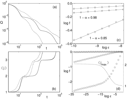
Figure 3: Chain model for $\xi_{1}=4.1$. (a) Survival probability $Q$ and (b) average position $\langle j\rangle$ as a function of time for $\mu=0.01$ and $\nu=0.02$ (full line), $\mu=0.01$ and $\nu=0.1$ (dashed, bottom), and $\mu=0.08$ and $\nu=0.1$ (dashed, top). (c) Fraction $f(\varepsilon)$ of uncertain points as a function of the scale $\varepsilon$ for points taken from $L=I_{1}$ (circles), $L=I_{2}$ (squares), and the subinterval $L$ of $I_{1}$ first mapped into $I_{2}$ (diamonds), where $\mu=0.01$ and $\nu=0.1$. Circles in (c) are shifted vertically upward for clarity. (d) The same as in (c) for $\varepsilon\geq 10^{-35}$ and $L=I_{1}$ (circles), $L=I_{2}$ (squares), and $L=I_{3}$ (triangles). Dashed line (right-side axis): average maximum $j$ of orbits started from $\varepsilon$-uncertain points, for $L=I_{1}$.

IV Effective Dynamical Invariants

Our results on the chain model motivate us to introduce the concept of effective dynamical invariants. As a specific example, we consider the effective fractal dimension, which, for the intersection of a fractal set $S$ with a $n$-dimensional region $L$, we define as

$$\left.D_{eff}(L;\varepsilon)=n-\frac{d\ln f(\varepsilon^{\prime})}{d\ln\varepsilon^{\prime}}\right|_{\varepsilon^{\prime}=\varepsilon},$$ (1)

where $f(\varepsilon^{\prime})=N(\varepsilon^{\prime})/N_{0}(\varepsilon^{\prime})$, and $N(\varepsilon^{\prime})$ and $N_{0}(\varepsilon^{\prime})$ are the number of cubes of edge length $\varepsilon^{\prime}$ needed to cover $S\cap L$ and $L$, respectively prev_work . We take $L$ to be a generic segment of line [i.e., $n=1$ in Eq. (1)] intersected by $S$ on a fractal set. In the limit $\varepsilon\rightarrow 0$, we recover the usual box-counting dimension $D=1-\lim_{\varepsilon\rightarrow 0}\Delta\ln f(\varepsilon)/\Delta\ln\varepsilon$ of the fractal set $S\cap L$, which is known to be 1 for all our choices of $L$. However, for any practical purpose, the parameter $\varepsilon$ is limited and cannot be made arbitrarily small (e.g., it cannot be smaller than the size of the particles, the resolution of the experiment, and the length scales neglected in modeling the system). At scale $\varepsilon$ the system behaves as if the fractal dimension were $D_{eff}(L;\varepsilon)$ (therefore “effective” dimension). In particular, the final state sensitivity of particles launched from $L$, with the initial conditions known within accuracy $\varepsilon^{*}$, is determined by $D_{eff}(L;\varepsilon^{*})$ rather than $D$: as $\varepsilon$ is variated around $\varepsilon^{*}$, the fraction of particles whose final state is uncertain scales as $\varepsilon^{1-D_{eff}(L;\varepsilon^{*})}$, which is different from the prediction $\varepsilon^{1-D}$. This is important in this context because, as shown in Fig. 3 (where the effective dimension is given by $1-\alpha$), the value of $D_{eff}(L;\varepsilon)$ may be significantly different from the asymptotic value $D=1$ even for unrealistically small $\varepsilon$ and may also depend on the region of the phase space. Similar considerations apply to many other invariants as well.

We now return to the Hamiltonian case. Consider a scattering process in which particles are launched from a line $L$ transversal to the stable manifold $W_{s}$ of the chaotic saddle. Based on the construction suggested by the chain model, it is not difficult to see that $W_{s}\cap L$ exhibits a hierarchical structure which is not self-similar and is composed of infinitely many nested Cantor sets, each of which is associated with the dynamics inside one of the regions $C_{j}$. As a consequence, the effective dimension $D_{eff}(L;\varepsilon)$ in Hamiltonian systems is expected to behave similarly to the effective dimension in the chain model [Figs. 3(c) and 3(d)]. In particular, $D_{eff}(L;\varepsilon)$ is expected to display a strong dependence on $L$ and a weak dependence on $\varepsilon$.

V Numerical Verification

We test our predictions on the area preserving Hénon map: $f(x,y)=(\lambda-y-x^{2},x)$, where $\lambda$ is the bifurcation parameter. In this system, typical points outside KAM islands are eventually mapped to infinity. Because of the symmetry $f^{-1}=g\circ f\circ g$, where $g(x,y)=(y,x)$, the stable and unstable manifolds of the chaotic saddle are obtained from each other by exchanging $x$ and $y$. For $\lambda=0.05$, the system displays a period-one and a period-four major island, as shown in Fig. 4(a). In the same figure we also show the complex invariant structure around the islands, the stable manifold of the chaotic saddle, and three different choices for the line of starting points: a large interval away from the islands ($L_{a}$), a small subinterval of this interval where the stable manifold appears to be denser ($L_{b}$), and an interval closer to the islands ($L_{c}$). The corresponding effective dimensions are computed for a wide interval of $\varepsilon$. The results are shown in Fig. 4(b): $D_{eff}(L_{a};\varepsilon)=0.84$, $D_{eff}(L_{b};\varepsilon)=0.90$, and $D_{eff}(L_{c};\varepsilon)=0.97$ for $10^{-8}<\varepsilon<10^{-5}$. These results agree with our predictions that the effective fractal dimension has the following properties: $D_{eff}$ may be significantly different from the asymptotic value $1$ of the fractal dimension; $D_{eff}$ depends on the resolution $\varepsilon$ but is nearly constant over decades; $D_{eff}$ depends on the region of the phase space under consideration and, in particular, is larger in regions closer to the islands and in regions where the stable manifold is denser. Similar results are expected for any typical Hamiltonian system with mixed phase space.

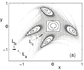
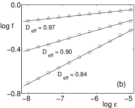
Figure 4: (a) KAM islands (blank), stable manifold (gray), and the lines of initial conditions ($L_{b}$ is a subinterval of $L_{a}$). (b) Effective dimension for $L=L_{a}$ (circles), $L=L_{b}$ (squares), and $L=L_{c}$ (triangles). The data in (b) are shifted vertically for clarity.

VI Conclusions

We have shown that the finite-scale dynamics of Hamiltonian systems, relevant for realistic situations, is governed by effective dynamical invariants. The effective invariants are not only different from the asymptotic invariants but also from the usual hyperbolic invariants because they strongly depend on the region of the phase space. Our results are generic and expected to meet many practical applications. In particular, our results are expected to be relevant for fluid flows, where the advection dynamics of tracer particles is often Hamiltonian fluid . In this context, a slow nonuniform convergence of effective invariants is expected not only for time-periodic flows, capable of holding KAM tori, but also for a wide class of time-irregular incompressible flows with nonslip obstacles or aperiodically moving vortices.

Appendix A

The diffusion model is: $\partial_{t}P(x,t)=\partial_{x}[x^{\alpha}\partial_{x}P(x,t)]$, where $P$ is the probability density of all particles, $x\geq 0$, and $\alpha>2$ chirikov1 . The outermost torus of the KAM island is at $x=0$, where the diffusion rate (proportional to $x^{\alpha}$) vanishes. In a chaotic scattering process the initial distribution of particles is localized apart from the confining islands. We take $P(x,0)=\delta(x-x_{0})$, $x_{0}>0$, and consider a particle to escape when it reaches $x\geq x_{1}$. Under the approximation that for large $x_{1}$ the return of particles can be neglected, we disregard the boundary condition $P(x_{1},t)=0$ and we take the solution to be the corresponding Green function: $P(x,t)=(\alpha-2)(xx_{0})^{-1/2}yy_{0}\exp(-y^{2}-y_{0}^{2})I_{\beta}(2yy_{0})$, where $y=(\alpha-2)^{-1}t^{-1/2}x^{-(\alpha-2)/2}$, $y_{0}$ is $y$ at $x=x_{0}$, $\beta=(\alpha-1)/(\alpha-2)$, and $I_{\beta}$ is the modified Bessel function, which scales as $I_{\beta}\sim(2yy_{0})^{\beta}$ for small $2yy_{0}$ greene1 . For any fixed $x>0$, we can show that the distribution for large $t$ decreases as $P(x,t)\sim t^{-\beta-1}$, where $\beta=(\alpha-1)/(\alpha-2)$. On the other hand, as shown in Ref. pikovsky1 , the fraction of particles in the interval $x<x_{1}$ decays algebraically as $Q(t)\equiv\int_{0}^{x_{1}}P(x,t)$d$x\sim t^{-\beta}$. Combining these two results, it follows that the normalized probability density $\rho(x,t)\equiv P(x,t)/Q(t)$ decreases as $\rho(x,t)\sim t^{-1}$ at each fixed $x\in(0,x_{1})$ for large enough $t$ and diverges arbitrarily close to $x=0$.

References

- (1) B. V. Chirikov, in Lecture Notes in Physics 179 (Springer, Berlin, 1983), pp. 29-46.
- (2) C. F. F. Karney, Physica D 8, 360 (1983); R. S. MacKay, J. D. Meiss, and I. C. Percival, Physica D 13, 55 (1984); B. V. Chirikov and D. L. Shepelyansky, Physica D 13, 395 (1984).
- (3) J. D. Meiss and E. Ott, Physica D 20, 387 (1986).
- (4) J. M. Greene, R. S. Mackay, and J. Stark, Physica D 21, 267 (1986).
- (5) A. S. Pikovsky, J. Phys. A: Math. Gen. 25, L477 (1992).
- (6) F. Christiansen and P. Grassberger, Phys. Lett. A 181, 47 (1993).
- (7) Y.-T. Lau, J. M. Finn, and E. Ott, Phys. Rev. Lett. 66, 978 (1991).
- (8) G. M. Zaslavsky, M. Edelman, and B. A. Niyazov, Chaos 7, 159 (1997); and references therein.
- (9) M. Weiss, L. Hufnagel, and R. Ketzmerick, Phys. Rev. E 67, 046209 (2003).
- (10) C. Jung, T. Tél, and E. Ziemniak, Chaos 3, 555 (1993).
- (11) J. C. Sommerer, H.-C. Ku, and H. E. Gilreath, Phys. Rev. Lett. 77, 5055 (1996).
- (12) R. Ketzmerick, Phys. Rev. B 54, 10841 (1996)
- (13) A. E. Motter and P. S. Letelier, Phys. Lett. A 285, 127 (2001).
- (14) Chain models have also been used to describe power laws generated by a hierarchy of repellers in the motion towards the Feigenbaum attractor [P. Grassberger and M. Scheunert, J. Stat. Phys. 26, 697 (1981)] and to study deterministic diffusion [R. Klages and J. R. Dorfman, Phys. Rev. Lett. 74, 387 (1995)].
- (15) Generalization to a full hierarchy of KAM islands is straightforward and does not change the essence of our results.
- (16) The escape rate follows from the same argument used in [J. D. Meiss and E. Ott, Physica D 20, 387 (1986)]. The fractal dimension follows from the observation that the dimension of the invariant set of map goes to as .
- (17) C. Grebogi, S. W. McDonald, E. Ott, and J. A. Yorke, Phys. Lett. A 99, 415 (1983).
- (18) D. Avnir, O. Biham, D. Lidar, and O. Malcai, Science 279, 39 (1998).
- (19) Different effective invariants have been introduced in Refs. finite1 . See also Refs. finite2 .
- (20) A. E. Motter, Y.-C. Lai, and C. Grebogi, Phys. Rev. E 68, 056307 (2003); A. P. S. de Moura and C. Grebogi, to be published.
- (21) Y.-C. Lai, M. Ding, C. Grebogi, and R. Blümel, Phys. Rev. A 46, 4661 (1992); W. Breymann, Z. Kovács, and T. Tél, Phys. Rev. E 50, 1994 (1994); P. Gaspard and J. R. Dorfman, Phys. Rev. E 52, 3525 (1995); V. Constantoudis and C. A. Nicolaides, Phys. Rev. E 64 056211 (2001).