Correlation Function Bootstrapping in Quantum Chaotic Systems

Abstract

We discuss a general and efficient approach for “bootstrapping” short-time correlation data in chaotic or complex quantum systems to obtain information about long-time dynamics and stationary properties, such as the local density of states. When the short-time data is sufficient to identify an individual quantum system, we obtain a systematic approximation for the spectrum and wave functions. Otherwise, we obtain statistical properties, including wave function intensity distributions, for an ensemble of all quantum systems sharing the given short-time correlations. The results are valid for open or closed systems, and are stable under perturbation of the short-time input data. Numerical examples include quantum maps and two-dimensional anharmonic oscillators.

I Introduction

When a quantum system is known to have a chaotic classical limit, the simplest description of its eigenvalues, eigenstates, and dynamics is given by the universal predictions of random matrix theory (RMT) rmt and the closely related random wave hypothesis berryrw . Recently, however, there has been increased interest in understanding the deviations from RMT that are quite sizable in many systems of interest and are often due to short-time dynamical effects. RMT assumes implicitly that under time evolution, any initial state immediately spreads randomly over the entire available Hilbert space; any realistic chaotic dynamics, however, maintains at short times information about the initial state and only after some finite mixing time $T_{\rm mix}$ does the dynamics become truly random.

For the purpose of describing spectral statistics, such as the distribution of level spacings, the above consideration may easily be taken into account by noting that RMT predictions are valid only inside energy windows of size less than a ballistic Thouless energy $E_{c}\sim\hbar/T_{\rm mix}$. The situation with wave functions is not so simple, as short-time dynamical effects can lead to large deviations from RMT not only for energy-averaged quasimodes but also for individual eigenstates.

Any short unstable periodic orbit is one obvious example of a non-random dynamical feature that is known to cause significant deviations from RMT statistics in the eigenstates. It has been shown that the “scarring” of individual wave functions by a typical periodic orbit is an $O(\hbar^{0})$ effect that persists in the semiclassical limit, as measured by the distribution of wave function intensities on the periodic orbit in Husimi phase space scarhusimi . Using a linearization of the dynamics around the specific orbit, the distribution of quantum intensities on or near the orbit may be obtained semiclassically as a function of the classical monodromy matrix, and various moments of the distribution, such as the inverse participation ratio, may be expressed analytically scarmom . The scarring effect has been studied experimentally and numerically in a wide variety of systems scareffect , and may have consequences for the conductance through a resonant tunneling diode or a ballistic quantum dot scardiode ; scarcond .

The imprint of short-time dynamics on eigenstate structure is not limited to situations where the short-time dynamics is related to classical unstable periodic orbits. For example, scar-like resonances related to diffractive trajectories have been observed in a 2DEG conductance experiment diffr . The approach of using short-time behavior to understand eigenstate structure and statistics has been used successfully in many situations where a proper classical limit does not exist, such as two-body random interactions in a many-fermion system papenbrock or dynamics on a quantum graph or lattice graphs , as well as in pseudo-integrable systems where the Lyapunov exponent vanishes superscar . Furthermore, short-time dynamical information necessarily implies deviations from RMT not only for individual wave function intensities, but also for spatial or phase space correlations schanz .

Our aim here is to discuss a systematic, general, and efficient framework for studying the constraints that short-time correlations impose on the eigenstate structure, regardless of whether such short-time correlations can be computed semiclassically. We allow ourselves to focus on one or an arbitrary number of initial wave packets, and the calculations may be performed equally well in closed or open systems, as there is no assumption of unitarity in the dynamics. We explicitly allow for the presence of errors in the short-time correlations, and demonstrate the stability of the results with respect to such errors.

In the context of extracting stationary properties from a time-domain correlation function, we mention the important work that has been done by Mandelshtam and coworkers using the “filter diagonalization” method mandelshtam . In that approach, one typically begins with a single wave packet, and spectral information can in principle be computed exactly when the correlation function is known for at least $N$ times, where $N$ is the Hilbert space dimension. In the bootstrapping approach, we use multiple initial wave packets, and we do not assume exact finite-dimensionality of the Hilbert space. Thus our goal is not an exact solution of the spectral analysis problem, but rather an increasingly good approximation as the amount of input data increases. Of course, exact solutions are not possible in any case in the presence of noise or numerical instability, so in practice regularization must be performed, yielding comparable results for the two approaches. One advantage of the bootstrapping approach is that the linear algebra involved requires $M\times M$ matrices only, where $M$ is the number of initial wave packets, allowing the problem to scale very well computationally for large system sizes and long times.

The paper is organized as follows. In Sec. II, we define the quantities of interest in the time and energy domain, and obtain general expressions for the bootstrapped correlation function and spectrum. Sec. III serves to define two sets of numerical models, which may be used to illustrate the general formalism. Next, in Sec. IV, we discuss convergence properties of the bootstrapping approximation, including a treatment of stability in the presence of noise. In Sec. V, we examine how bootstrapping may be used to compute statistical quantities of interest, including wave function intensity distributions and intensity correlations, using a very small amount of time-domain data as input. Finally, the key conclusions are briefly summarized in Sec. VI.

II Bootstrapping for Correlation Functions and Spectrum

We begin by considering a set of $M$ wave packets $\phi_{i}$, for simplicity taking the wave packets to be orthonormal (but not a complete set). In practice, the choice of $\phi_{i}$ will be dictated by the physics of interest. For example, the $\phi_{i}$ may be chosen as position eigenstates if we are interested in position-space wave function structure, or momentum eigenstates for scattering behavior, or Gaussian wave packets for analyzing the effects of classical periodic orbits. In a many-body problem, the $\phi_{i}$ may usefully be taken as the non-interacting product states.

The quantity of interest in the time domain is the correlation function

$$C_{ij}(t)=\langle\phi_{i}|e^{-i\hat{H}t/\hbar}|\phi_{j}\rangle\,,$$ (1)

whose diagonal elements $C_{ii}(t)$ constitute the autocorrelation functions for the individual wave packets. Knowledge of the exact correlation function for all discrete times $t=mT_{0}$ leads by Laplace transform to the discrete-time Green’s function

$$G_{ij}(E) = (i\hbar)^{-1}T_{0}\sum_{m=0}^{\infty}\left[e^{iEmT_{0}/\hbar}-{1\over 2}\delta_{m0}\right]C_{ij}(mT_{0})=(i\hbar)^{-1}T_{0}\langle\phi_{i}|{1\over 1-e^{i(E-\hat{H})T_{0}/\hbar}}-{1\over 2}|\phi_{j}\rangle$$ (2)

$$\approx (i\hbar)^{-1}\int_{0}^{\infty}dt\;e^{iEt/\hbar}C_{ij}(t)=\langle\phi_{i}|{1\over E-\hat{H}+i\epsilon}|\phi_{j}\rangle\,,$$ (3)

where the continuous-time limit of Eq. (3) is obtained for $T_{0}\ll\hbar/\delta E$, and $\delta E$ is a typical energy spread in the wave packets.

We will see that it proves useful to decompose the return amplitude of Eq. (1) at time $t$ into a special “new” component that is returning for the first time to the subspace spanned by the $M$ wave packets $\phi_{i}$ and the remainder due to propagation that has revisited this subspace at least once at time steps in between $0$ and $t$. In spirit, this is reminiscent of the $T-$matrix approach of Bogomolny tmatrix , where an integral kernel is defined in terms of all classical trajectories that start on a given Poincaré surface of section and return to the surface of section without intersecting it at intermediate times. The $T-$matrix is defined directly in the energy domain whereas we begin our analysis in the time domain and transform to the energy domain later on. The decomposition used here also resembles somewhat the one used in the quantitative analysis of periodic orbit scarring scarhusimi , where it is helpful to separate terms in the return amplitude that are associated with paths staying on the periodic orbit from terms associated with homoclinic paths that leave the orbit once and first return at some later time. Of course, in the case we consider here the $M-$dimensional subspace spanned by the wave packets $\phi_{i}$ will not in general have any connection with a particular classical structure such as a periodic orbit or surface of section. Instead the choice of $\phi_{i}$ is governed either by our exact or approximate knowledge of the correlation function for those initial and final states or by an interest in extracting wave function structure information in a specific basis or phase space region. Furthermore, no semiclassical approximation is implicit in the method we develop here, although we will see below that the approach can be extended to situations where the correlation function information used as input is only approximate, as would be the case for example when a semiclassical propagator is used.

Formally, the new recurrences $B_{ij}(m)$ at time $t=mT_{0}$ may be defined as

$$B_{ij}(m)=\langle\phi_{i}|e^{-i\hat{H}T_{0}/\hbar}\left((1-\hat{P})e^{-i\hat{H}T_{0}/\hbar}\right)^{m-1}|\phi_{j}\rangle\,,$$ (4)

where

$$\hat{P}=\sum_{k=1}^{M}|\phi_{k}\rangle\langle\phi_{k}|$$ (5)

is the projection onto the subspace of interest. More explicitly, these new recurrences may be computed from the full $C_{ij}$ amplitudes as

$$B_{ij}(m)=\left\{\begin{array}[]{ll}C_{ij}(T_{0})&m=1\\ C_{ij}(mT_{0})-\sum_{p=1}^{m-1}\sum_{k=1}^{M}B_{ik}(p)C_{kj}((m-p)T_{0})&m\geq 2\end{array}\right.\,.$$ (6)

The full correlation function is then given by a convolution,

$$C_{ij}(mT_{0})=\sum_{p=1}^{m}\sum_{k=1}^{M}B_{ik}(p)C_{kj}((m-p)T_{0})$$ (7)

or, in matrix notation,

$${\mathbf{C}}(mT_{0}) = \sum_{p=1}^{m}{\mathbf{B}}(p){\mathbf{C}}((m-p)T_{0})$$ (8)

$$= {\mathbf{B}}(m)+\sum_{p=1}^{m-1}{\mathbf{B}}(p){\mathbf{B}}(m-p)+\sum_{p=1}^{m-2}\sum_{p^{\prime}=1}^{m-p-1}{\mathbf{B}}(p){\mathbf{B}}(p^{\prime}){\mathbf{B}}(m-p-p^{\prime})+\cdots\,,$$

where ${\mathbf{C}}(0)$ is always the identity matrix. The matrix ${\mathbf{B}}(m)$ records amplitude that at the $m-$th step returns for the first time to the subspace spanned by the $\phi_{i}$, while terms in Eq. (8) involving a product of $n$ $\mathbf{B}$-matrices correspond to processes where amplitude leaves and returns $n$ times to the same subspace over $m$ steps. In the energy domain,

$$G_{ij}(E)=(i\hbar)^{-1}T_{0}\langle\phi_{i}|{1\over 1-{\mathbf{\tilde{B}}}(E)}-{1\over 2}|\phi_{j}\rangle\,,$$ (9)

where

$${\mathbf{\tilde{B}}}(E)=\sum_{m=1}^{\infty}e^{imT_{0}E/\hbar}{\mathbf{B}}(m)\,.$$ (10)

We are however interested in the information that can be extracted from knowledge of the correlation function at a finite set of times $t$ only, say $t=mT_{0}$ for $m=1\cdots L$, possibly in the presence of noise. If we assume ${\mathbf{C}}(mT_{0})$ is known only for times $t\leq T_{\rm max}=LT_{0}$, i.e., for $1\leq m\leq L$, then we may compute the new recurrences ${\mathbf{B}}(mT_{0})$ only for $1\leq m\leq L$ using Eq. (6). It is convenient to define

$${\mathbf{B}}_{L,\tau}(m)=\left\{\begin{array}[]{ll}{\mathbf{B}}(m)e^{-mT_{0}/\tau}&1\leq m\leq L\\ 0&{\rm otherwise}\end{array}\right.\,.$$ (11)

The cutoff time $\tau$, which can be much larger than the bootstrap time $T_{\rm max}=LT_{0}$, serves as a smoothing scale in the energy domain, and its significance will be discussed in Sec. IV below. Given just the matrices ${\mathbf{B}}_{L,\tau}(m)$, we may compute a “bootstrapped” approximation to the full correlation function at all times:

$${\mathbf{C}}_{L,\tau}(mT_{0}) = \sum_{p=1}^{m}{\mathbf{B}}_{L,\tau}(p){\mathbf{C}}_{L,\tau}((m-p)T_{0})$$ (12)

$$= {\mathbf{B}}_{L,\tau}(m)+\sum_{p=1}^{m-1}{\mathbf{B}}_{L,\tau}(p){\mathbf{B}}_{L,\tau}(m-p)+\sum_{p=1}^{m-2}\sum_{p^{\prime}=1}^{m-p-1}{\mathbf{B}}_{L,\tau}(p){\mathbf{B}}_{L,\tau}(p^{\prime}){\mathbf{B}}_{L,\tau}(m-p-p^{\prime})+\cdots\,,$$

having the property ${\mathbf{C}}_{L,\tau}(mT_{0})={\mathbf{C}}(mT_{0})e^{-mT_{0}/\tau}$ for $m\leq L$. In the energy domain, ${\mathbf{\tilde{B}}}_{L,\tau}(E)$ may be defined as a Laplace transform of ${\mathbf{B}}_{L,\tau}(m)$, in complete analogy with Eq. (10) above.

Finally, one often encounters a “noisy” situation where even the short-time dynamics is only approximately known. For example, we may be interested in building up the full dynamics using only semiclassical expressions for the propagator at short times. We then have knowledge of

$${\mathbf{C}}_{\epsilon}(mT_{0})={\mathbf{C}}(mT_{0})+\epsilon{\mathbf{D}}(mT_{0})$$ (13)

for $1\leq m\leq L$, where ${\mathbf{D}}(mT_{0})$ are quasi-random, uncorrelated error matrices and $\epsilon$ characterizes the relative size of the error. Given this input data we may calculate approximate “new” recurrences ${\mathbf{B}}_{L,\tau,\epsilon}(mT_{0})$ by extending the exact formula of Eq. (6),

$${\mathbf{B}}_{L,\tau,\epsilon}(m)=\left\{\begin{array}[]{ll}{\mathbf{C}}_{\epsilon}(T_{0})e^{-T_{0}/\tau}&m=1\\ {\mathbf{C}}_{\epsilon}(mT_{0})e^{-mT_{0}/\tau}-\sum_{p=1}^{m-1}{\mathbf{B}}_{L,\tau,\epsilon}(p){\mathbf{C}}_{\epsilon}((m-p)T_{0})e^{-(m-p)T_{0}/\tau}&2\leq m\leq L\\ 0&{\rm otherwise}\end{array}\right.\,.$$ (14)

The “bootstrapped” long-time evolution ${\mathbf{C}}_{L,\tau,\epsilon}$ is given by iterating these approximately known short-time “new” recurrences analogously to Eq. (12),

$${\mathbf{C}}_{L,\tau,\epsilon}(mT_{0}) = \sum_{p=1}^{m}{\mathbf{B}}_{L,\tau,\epsilon}(p){\mathbf{C}}_{L,\tau,\epsilon}((m-p)T_{0})$$ (15)

$$= {\mathbf{B}}_{L,\tau,\epsilon}(m)+\sum_{p=1}^{m-1}{\mathbf{B}}_{L,\tau,\epsilon}(p){\mathbf{B}}_{L,\tau,\epsilon}(m-p)+\sum_{p=1}^{m-2}\sum_{p^{\prime}=1}^{m-p-1}{\mathbf{B}}_{L,\tau,\epsilon}(p){\mathbf{B}}_{L,\tau,\epsilon}(p^{\prime}){\mathbf{B}}_{L,\tau,\epsilon}(m-p-p^{\prime})+\cdots\,.$$

Again, by construction the bootstrapping procedure simply reproduces the noisy input data for times $t$ below the bootstrap time $T_{\rm max}$, i.e., ${\mathbf{C}}_{L,\tau,\epsilon}={\mathbf{C}}_{\epsilon}e^{-mT_{0}/\tau}$ for $m\leq L$. However, bootstrapping allows us also to learn something about longer times $t>T_{\rm max}$ using the short-time correlation function.

III Numerical Models

III.1 Quantum Maps

Classical and quantum chaotic maps in one dimension are often used as the simplest examples for illustrating general chaotic behavior, and share many scaling and other physical properties of two-dimensional Hamiltonian dynamics maps . Discrete-time maps may be thought of as arising from a continuous-time Hamiltonian dynamics either via a Poincaré surface of section or by stroboscopically viewing motion in a periodically driven Hamiltonian. In the latter case, we may consider

$$H(q,p,t)={1\over T_{\rm kick}}T(p)+V(q)\sum_{j=-\infty}^{\infty}\delta(t-jT_{\rm kick})\,,$$ (16)

which yields

$$p_{j+1} = p_{j}-V^{\prime}(q_{j})$$

$$q_{j+1} = q_{j}+T^{\prime}(p_{j+1})\,,$$ (17)

when the position $q_{j}$ and momentum $p_{j}$ are recorded just before kick $j$. The corresponding quantum evolution over one time step is given by

$$\hat{U}=e^{-iT(\hat{p})/\hbar}e^{-iV(\hat{q})/\hbar}\,.$$ (18)

As a specific example, we may take $T(p)={1\over 2}w_{p}p^{2}+K_{p}(\sin{p}-{1\over 2}\sin{2p})$ and $V(q)=-{1\over 2}w_{q}q^{2}-K_{q}(\sin{q}-{1\over 2}\sin{2q})$, for a toral phase space $(q,p)\in[-\pi 0,\pi)\times[-\pi,\pi)$. With integer values of $w_{q}$ and $w_{p}$, this is a perturbed cat map pertcat :

$$p_{j+1} = p_{j}+w_{q}q_{j}+K_{q}(\cos{q_{j}}-\cos{2q_{j}})\;\;{\rm mod}\;\;2\pi$$

$$q_{j+1} = q_{j}+w_{p}p_{j}+K_{p}(\cos{p_{j}}-\cos{2p_{j}})\;\;{\rm mod}\;\;2\pi\,,$$ (19)

where nonzero values of $K_{q}$, $K_{p}$ are needed to break the symmetries and ensure nonlinearity of the dynamics. One easily checks that the dynamics is completely chaotic for sufficiently small $K_{q,p}$.

For this compact classical phase space, the quantum evolution of Eq. (18) acts on a Hilbert space of dimension $N=2\pi/\hbar$, the mean energy level spacing is $\Delta=2\pi\hbar/NT_{\rm kick}=\hbar^{2}/T_{\rm kick}$, and the Heisenberg time at which levels are resolved is $T_{H}=NT_{\rm kick}$. Since the map dynamics is already discretized, it is natural to use the period $T_{\rm kick}$ as the time step $T_{0}$ in the bootstrapping calculation. Without loss of generality, we may choose units where $T_{0}=T_{\rm kick}=1$.

III.2 Two-Dimensional Wells

As our model of a non-integrable system with a time-independent Hamiltonian, we use the Barbanis Hamiltonian barbanis , which describes a two-dimensional anharmonic oscillator:

$$H(x^{\prime},y^{\prime},{p^{\prime}}_{x},{p^{\prime}}_{y})={{p^{\prime}}_{x}^{2}\over 2m}+{{p^{\prime}}_{y}^{2}\over 2m}+{1\over 2}m\omega_{x}^{2}x^{\prime 2}+{1\over 2}m\omega_{y}^{2}y^{\prime 2}+\lambda x^{\prime}{y^{\prime}}^{2}\,.$$ (20)

After a canonical transformation and an overall rescaling of the energy, the Barbanis Hamiltonian may be re-written as

$$H(x,y,p_{x},p_{y})={p_{x}^{2}\over 2}+{p_{y}^{2}\over 2}+{1\over 2}x^{2}+{a\over 2}y^{2}+{a\over 2}xy^{2}\,,$$ (21)

where $a$ is a dimensionless parameter characterizing the shape of the well. In these dimensionless coordinates, the metastable well has its minimum at $x=y=0$ and extends from $x=-1$ to $x=1$ along the $y=0$ symmetry axis; the barrier height is $E_{\rm max}=1/2$. Upon quantization, one additional parameter besides $a$ is introduced, namely an effective $\hbar$ or equivalently the number of quantum levels below $E_{\rm max}$.

As compared with the simple quantum map model presented above, analysis of bootstrapping in the Barbanis system requires consideration of the following three circumstances, which are typical of many Hamiltonian systems: (i) time is not naturally discrete and thus an explicit choice is needed for the discretization time $T_{0}$, (ii) resonances in the metastable well have finite intrinsic width, introducing a new long-time scale, and (iii) classical dynamics in the well is mixed, with the phase space at energies of interest shared by regular islands and a chaotic sea. The implications of these three circumstances will be discussed below, when numerical results for bootstrapping in the Barbanis system are presented in Sec. IV.2.

IV Convergence Properties and Sensitivity to Error

In this section, we examine how bootstrapping may be used when the given information about the short-time correlation function is sufficient to compute (approximately) the long-time dynamics and spectrum. An alternative situation, where the given information only restricts us to an ensemble of possible long-time behaviors, and the objective is to obtain statistical properties of the long-time dynamics or spectrum, is discussed in Sec. V.

IV.1 Noise-Free Bootstrapping

We want to estimate the error made in using short-time information up to the bootstrap time $T_{\rm max}=LT_{0}$ to estimate long-time dynamics in a chaotic system at times $t\gg T_{\rm max}$. Let us first assume negligible noise by setting $\epsilon=0$ in Eq. (13). Clearly the error is then associated with amplitude that starts in the subspace spanned by the $M$ wave packets $\phi_{i}$ and is never captured by the short-time correlation function because it does not return to the original subspace at any time during the first $L$ steps of evolution. In terms of the ${\mathbf{B}}-$matrices discussed in the previous section, the total probability that does not return in time $T_{\rm max}=LT_{0}$ is

$$P(T_{\rm max})=1-{1\over M}\sum_{m=1}^{L}{\rm Tr}\;{\mathbf{B}}(m)^{\dagger}{\mathbf{B}}(m)\,.$$ (22)

Mathematically, the probability $P(T_{\rm max})$ is clearly related to the probability of remaining for at least time $T_{\rm max}$ in a system with $M$ maximally coupled open decay channels. When the dynamics is chaotic, this probability can be represented analytically as an integral in the context of random matrix theory savin ; for our purposes it is sufficient to note that

$$P(T_{\rm max})=\left\{\begin{array}[]{ll}e^{-MT_{\rm max}/T_{H}}&T_{\rm max}\ll T_{H}/\sqrt{M}\\ {1\over M+1}\left({T_{H}/T_{\rm max}}\right)^{M+1}&T_{\rm max}\gg T_{H}\end{array}\right.\,,$$ (23)

where $T_{H}$ is the Heisenberg time, and the power-law long-time limit also serves as an upper bound for $P(T_{\rm max})$. Clearly, we require $T_{\rm max}>T_{H}/M$ in order to recapture most of the initial amplitude, so that the lost probability is small. We emphasize that this estimate, based on random matrix theory, may be used to obtain the correct scaling behavior of the lost probability $P(T_{\rm max})$ with bootstrap time $T_{\rm max}$, even when the prefactor in Eq. (23) is invalid due to nonrandom short-time dynamical effects.

Figure 1: The lost probability $P(T_{\rm max})$ associated with eliminating new recurrences arriving after time $T_{\rm max}$ is plotted as a function of $T_{\rm max}$ for the quantum map of Eq. (19), with $w_{q}=w_{p}=1$ and parameters $K_{q}$, $K_{p}$ uniformly distributed between $-1/2$ and $1/2$. Squares, circles, and triangles represent data when the number of wave packets $M$ is $M=1$, $2$, or $4$, respectively. Open symbols are associated with system size $N=64$ and closed symbols with system size $N=128$. The dashed curve is the small-$T_{\rm max}$ (classical) limit in Eq. (23), while the three solid lines represent the large-$T_{\rm max}$ power-law falloff for $M=1$, $2$, and $4$. All quantities shown in this and subsequent figures are dimensionless.

The behavior of the lost probability $P(T_{\rm max})$ for small and large $T_{\rm max}$ is illustrated in Fig. 1. Here an average over quantum maps given by Eq. (19) has been performed, with $w_{q}=w_{p}=1$ and nonlinearity parameters $K_{q}$, $K_{p}$ randomly distributed between $-1/2$ and $+1/2$. We note the expected exponential behavior for small $T_{\rm max}$, with the classical decay rate $M/T_{H}$, as well as the rapid power-law decay of the lost probability for $T_{\rm max}>T_{H}$, especially in the case of multiple wave packets $M>1$.

We are interested in the error induced at long times $t\gg T_{\rm max}$ by omitting new recurrences not captured in the short-time correlation function. At this point, we have not introduced any smoothing of the input data, i.e., $\tau=\infty$ in Eq. (11). The typical returning amplitude at time $t$ has completed $O(Mt/T_{H})$ cycles of leaving and returning to the subspace spanned by the $M$ wave packets $\phi_{i}$, i.e., in Eq. (8) the dominant terms are ones involving a product of $O(Mt/T_{H})$ ${\mathbf{B}}-$matrices. In each cycle, probability given by Eq. (23) is lost, with the errors accumulating coherently, so that the relative error in the matrix elements at time $t\gg T_{\rm max}=LT_{0}\geq T_{H}/M$ is given by

$$E(t)={||{\mathbf{C}}_{L,\infty}(t)-{\mathbf{C}}(t)||^{2}\over||{\mathbf{C}}(t)||^{2}}\sim\left({Mt\over T_{H}}\right)^{2}P(T_{\rm max})\,,$$ (24)

where $||{\mathbf{C}}(t)||^{2}={\rm Tr}\;{\mathbf{C}}(t)^{\dagger}{\mathbf{C}}(t)=\sum_{ij}|C_{ij}(t)|^{2}$. The quadratic growth in the long-time error is clearly seen in Fig. 2 for several choices of the bootstrapping parameters.

Figure 2: The ratio of the relative error in the propagator, $E(t)$, to the probability lost on average during each cycle of recurrences, $P(T_{\rm max})$, is plotted for times $t>T_{\rm max}$, $M=2$, several values of $T_{\rm max}$, and two system sizes. All system parameters are the same as in the previous figure. Squares, circles, and triangles correspond to $MT_{\rm max}/T_{H}=5$, $10$, and $20$, respectively, while open and closed symbols distinguish system size $N=64$ from system size $N=128$. The solid line indicates the quadratic growth of the error consistent with Eq. (24).

To find the time scale $T_{\rm break}$ beyond which the bootstrapping procedure breaks down, we assume $T_{H}/M\leq T_{\rm max}\leq T_{H}/\sqrt{M}$. Then, setting the right hand side of Eq. (24) to unity and using Eq. (23), we obtain

$$T_{\rm break}\sim T_{\rm max}{\exp{({1\over 2}MT_{\rm max}/T_{H}})\over MT_{\rm max}/T_{H}}\,.$$ (25)

We see that including only a minimal number of new recurrences by setting $T_{\rm max}\sim T_{H}/M$ leads to breakdown of the bootstrapping approximation soon thereafter ($T_{\rm break}\sim T_{\rm max}$), but including additional recurrences leads to exponential growth in the accuracy of the bootstrapping approximation and consequently to exponential increase in the breakdown time. Of course, this exponential growth ceases at very large values of $T_{\rm max}$, when the error becomes dominated by a small fraction of eigenstates that have unusually little overlap with the wave packets $\phi_{i}$. Then $P(T_{\rm max})$ follows the power-law behavior of Eq. (23), and the growth in $T_{\rm break}$ accordingly crosses over to a power-law behavior with $T_{\rm max}$:

$$T_{\rm break}\sim T_{H}{\sqrt{M+1}\over M}\left({T_{\rm max}\over T_{H}}\right)^{M+1\over 2}$$ (26)

for $T_{\rm max}>T_{H}$. We note that the growth of the break time $T_{\rm break}$ with increasing bootstrap time $T_{\rm max}$ remains faster than linear except in the single-wave packet case $M=1$. This super-linear growth is illustrated in Fig. 3 for the case of two wave packets ($M=2$), where the break time $T_{\rm break}$ has been quantified as the time scale where the relative error of Eq. (24) reaches unity.

Figure 3: The break time $T_{\rm break}$ of the bootstrapping approximation, defined by $E(T_{\rm break})=1$, is plotted for $M=2$ and several choices of $T_{\rm max}$. Open and closed squares represent system sizes $N=64$ and $N=128$, respectively. The ensemble of systems is the same as in the previous two figures. The straight line is the theoretical prediction $T_{\rm break}\sim T_{\rm max}^{(M+1)/2}\sim T_{\rm max}^{3/2}$ of Eq. (26).

IV.2 Results in the Energy Domain

Starting with known short-time information about the correlation function, the bootstrapped long-time dynamics may be Laplace or Fourier transformed into the energy domain to obtain good approximations to the Green’s function, spectrum, or local density of states. Alternatively, the short-time “new” recurrences may be transformed directly into the energy domain to obtain spectral information, as indicated by Eqs. (9) and (10). To avoid unphysical oscillations in the spectrum on energy scales below $\hbar/T_{\rm break}$ (associated with the breakdown of the bootstrapping approximation at long times), we impose an explicit smooth cutoff on the the short-time dynamics, in accordance with Eq. (11). Loss of information is minimized by choosing the cutoff time $\tau$ of the order of $T_{\rm break}$, which is equivalent to Lorentzian smoothing of the spectrum on the scale $\hbar/T_{\rm break}$.

The numerical data presented in Fig. 4 is obtained for the Barbanis potential, with parameters $a=1.1$ and $\hbar=0.0198$ in Eq. (21), corresponding to slightly over $300$ quantum resonances in the metastable well. Six initial Gaussian wave packets are used in the calculation, all centered at $x=0$ and having an average momentum of magnitude $|p|=0.96$, corresponding to an energy $E=0.46$. Thus, we are viewing dynamics slightly below the top of the barrier, $E_{\rm max}=0.5$. The classical dynamics in the energy range considered is approximately $57\%$ chaotic, as measured using a Poincaré surface of section at $x=0$. All six initial wave packets are centered in the chaotic region of classical phase space.

Figure 4: The local density of states summed over $M=6$ wave packets located at energy $E=0.46$ in the Barbanis potential of Eq. (21), $S(E)=\sum_{j=1}^{6}{\rm Re}\;(i/\pi)\,G_{jj}(E)$, is computed using the bootstrapping approximation in accordance with Eq. (9). The three solid curves from bottom to top correspond to different bootstrap times used in the bootstrapping calculation: $T_{\rm max}=T_{H}/2$, $T_{\rm max}=T_{H}$, and $T_{\rm max}=2T_{H}$. For comparison, the result of Laplace transforming the correlation function through time $T_{\rm max}=2T_{H}$, without bootstrapping, is shown as a dashed curve. Each spectrum has been scaled by an arbitrary constant to allow for easy comparison on a single plot. In each case a smoothing time scale $\tau\sim T_{\rm break}$ has been chosen to remove unphysical oscillations in the spectrum in the energy range shown. The dotted vertical lines indicate the locations of the exact resonance peaks, obtained by taking $T_{\rm max}\to\infty$.

We see from the middle solid curve in Fig. 4 that most peaks in the spectrum can readily be resolved using bootstrapping, taking correlation information up through the Heisenberg time $T_{H}$ as our only input. For bootstrap time $T_{\rm max}=2T_{H}$ (top solid curve), the spectral peak heights already stand out by four orders of magnitude above the background. The root mean squared error in the bootstrap-predicted peak locations drops from $0.034\Delta$ when $T_{\max}=T_{H}$ to $0.0064\Delta$ for $T_{\rm max}=2T_{H}$, where $\Delta$ is the mean level spacing. We may contrast this with the result, indicated by the dashed curve, of merely transforming and smoothing the same correlation information, up through $T_{\rm max}=2T_{H}$, but without the benefit of bootstrapping. Here the resolution is very poor, and we are far from being able to detect, for instance, the two doublets near $E=0.4515$ and $E=0.4535$.

In contrast with the map model studied in Section IV.1, in the Hamiltonian system investigated here we must discretize time explicitly by introducing a new time scale $T_{0}$. The results of the calculation, however, are unaffected by the choice of $T_{0}$, as long as $T_{0}<\hbar/\delta E$, where $\delta E$ is the energy uncertainty in the wave packets $\phi_{i}$. Equivalently, the time step $T_{0}$ must be chosen short enough so that the self-overlaps $C_{ii}(T_{0})$ are large due to free-flight dynamics.

A second key difference with the map model is that quantum motion in the Barbanis potential is described by resonances rather than bound states. Indeed, by comparing the upper two curves in Fig. 4, we see that in the $T_{\rm max}=T_{H}$ bootstrapped spectrum, the widths of several peaks (e.g., the rightmost one near $E=0.4612$) are already dominated by the intrinsic resonance widths rather than by any error associated with the time cutoff. In general, the efficiency of the bootstrapping approach increases as one considers systems that are more open, since it is sufficient to choose a bootstrap time $T_{\rm max}$ that will generate accurate dynamics to time $T_{\rm break}\sim T_{\rm decay}$, where $T_{\rm decay}$ is the intrinsic lifetime of the resonances, possibly shorter than $T_{H}$.

Finally, a third major difference between perturbed cat maps and the Barbanis potential is the presence of regular as well as chaotic states in the Barbanis spectrum. By choosing the test wave packets $\phi_{i}$ appropriately, one may optimally resolve states in the phase space region that are of greatest interest in a given application. For example, in ordinary scar theory, one may begin with a wave packet centered on a specific periodic orbit scarhusimi , with the aim of obtaining optimal information on the structure of wave functions with high intensity on that orbit and their associated eigenvalues; the price to be paid is the suppression of the “anti-scarred” eigenstates that have anomalously low intensity on the same orbit. Here, we have randomly placed the six test wave packets in the chaotic portion of phase space, improving our ability to resolve the chaotic states, but necessitating the use of longer bootstrap times $T_{\rm max}$ to identify spectral peaks associated with regular wave functions, such as the very narrow resonance peak near $E=0.4536$.

In this context we note also that, in the case of scar theory, little or no benefit is gained by following several wave packets launched along the same weakly unstable periodic orbit, since they all exhibit very similar time evolution, and share nearly identical local density of states scarmometer . From a bootstrapping perspective, we may consider two wave packets nearly related by time evolution, e.g., $|\phi_{2}\rangle\approx e^{-i\hat{H}\tau/\hbar}|\phi_{1}\rangle$. Then the probability $1-P(T_{\rm max})$ of Eq. (22) for returning to the subspace spanned by $\phi_{1}$ and $\phi_{2}$ by time $T_{\rm max}$ is nearly the same as the probability of returning to $\phi_{1}$ itself, assuming $T_{\rm max}\gg\tau$. The rapid decrease in the “lost probability” $P(T_{\rm max})$ with increasing number of wave packets $M$, as indicated by Eq. (23), depends entirely on the wave packets behaving in an uncorrelated manner. Thus, the bootstrapping procedure for multiple wave packets is most effective when the wave packets are chosen from different regions of phase space to avoid obvious correlations.

IV.3 Influence of Noise

Noise in the input signal may be an important factor in specific applications of the bootstrapping procedure, for example where a semiclassical or other approximation is used to calculate the short-time correlation function. We return to the quantum map model discussed in Sec. IV.1 and introduce random noise into the short-time correlation function, as indicated in Eq. (13). The random error matrix elements $D_{ij}(m)$ in Eq. (13) are independent Gaussian random variables of zero mean and variance $1/N$, where $N$ is the Hilbert space dimension, so that $\overline{|D_{ij}(m)|^{2}}=\overline{|C_{ij}(m)|^{2}}$ at long times $m$. Then the dimensionless parameter $\epsilon$ characterizes the relative size of the noise. A spectrum may be produced by bootstrapping the noisy short-time data. The results of such a calculation are presented in Fig. 5. We see that the spectral reconstruction is quite robust for small $\epsilon$, and breaks down at around $\epsilon=0.2$ or $0.3$, independent of $N$ and $M$.

Figure 5: The local density of states summed over $M$ randomly placed wave packets, $S(E)=\sum_{j=1}^{M}{\rm Re}\;(i/\pi)\,G_{jj}(E)$, is computed for the quantum map of Eq. (19), with $w_{q}=w_{p}=1$, $K_{q}=0.2$, and $K_{p}=-0.3$, using the bootstrapping approximation after noise has been introduced into the short-time input data. From top to bottom, the three sets of curves correspond to (a) $N=128$, $M=2$, (b) $N=128$, $M=6$, and (c) $N=512$, $M=2$, where $N$ is the system size or Hilbert space dimension. Within each set, the top (solid) curve is the reconstructed spectrum in the absence of noise, and the three dashed/dotted curves, from upper to lower, indicate reconstructed spectra for the same system with the dimensionless noise parameter set to $\epsilon=0.1$, $\epsilon=0.2$, and $\epsilon=0.3$. Each spectrum has been scaled by an arbitrary constant to allow for easy comparison on a single plot. In all cases, the spectrum is reconstructed from the correlation function for $t\leq T_{\rm max}=3T_{H}/M$.

To study more carefully the breakdown in the accuracy of the bootstrapped spectrum and its dependence on parameters $N$ and $M$, we need to define a quantitative measure of the error in the bootstrapped spectrum. Consider a local density of states $S(E)$ reconstructed from the exact correlation function known for $t\leq T_{\rm max}$ and a local density of states $S_{\epsilon}(E)$ reconstructed from the same input but with added noise characterized by $\epsilon$ as in Eq. (13). We may define the dimensionless error ratio

$$Z(\epsilon)={\int dE\,(\ln S_{\epsilon}(E)-\ln S(E))^{2}\over\int dE\,(\ln S(E))^{2}}\,,$$ (27)

which measures the error induced in the reconstructed spectrum by noise of size $\epsilon$ in the input. We note that it is appropriate to focus on the logarithm of the reconstructed spectrum, because the spectrum itself is dominated by sharp peaks, as seen in Fig. 5. The quantity $Z(\epsilon)$ is shown in Fig. 6, for the same parameters as were used earlier in Fig. 5. Not surprisingly, we observe growth in the spectral error with increasing noise $\epsilon$, but, more importantly, this error is almost independent of system size $N$ and number of wave packets $M$ (at $\epsilon=0.3$, $Z(\epsilon)$ varies at most by $30\%$ as $N$ changes by a factor of $4$ and $M$ by a factor of $3$). The same results have been observed for other system parameters. This robustness implies that input with noise of a small but finite size $\epsilon$ may be used in the semiclassical limit $N\to\infty$ (equivalently, $\hbar\to 0$). Obviously, an even more favorable situation exists when the noise level $\epsilon$ decreases with increasing $N$. An important example of the latter situation exists when the “noise” results from using a semiclassical (stationary phase) approximation for the short-time dynamics $t\leq T_{\rm max}$. Then $\epsilon\sim\hbar$, which decreases with $N$. Therefore short-time evolution computed within a semiclassical approximation may be used with confidence to obtain stationary properties of the exact quantum system.

Figure 6: The error $Z(\epsilon)$ in the reconstructed spectrum for the quantum map of Eq. (19) is computed as a function of the noise level $\epsilon$ in the input correlation function. All parameters are identical to those in Fig. 5. The solid curve indicates system size $N=128$ with $M=2$ wave packets, the dashed curve is for $N=512$ with $M=2$, and the dotted curve is for $N=128$ with $M=6$. In all cases, the noise-free spectrum $S(E)$ and the noisy spectrum $S_{\epsilon}(E)$ are both reconstructed from the correlation function for $t\leq T_{\rm max}=3T_{H}/M$.

V Bootstrapped Wave Function Statistics

We now consider the situation where known short-time dynamical information is insufficient for resolving individual eigenstates, and the focus therefore shifts to predictions of a statistical nature. In other words, we consider an ensemble of systems that all share (perhaps approximately) a given short-time dynamics, and ask what information can be extracted about the distribution of wave functions in systems drawn from this ensemble.

V.1 Inverse Participation Ratio Calculations

The simplest quantitative measure of wave function structure is the inverse participation ratio (IPR) or second moment of the wave function intensities ipr : ${\rm IPR}_{\Psi}=N\sum_{i=1}^{N}|\langle\phi_{i}|\Psi\rangle|^{4}$, where $\Psi$ is an eigenstate, $N$ is the Hilbert space dimension, the sum is over a complete basis $\phi_{i}$, and we impose the usual normalization condition $\sum_{i=1}^{N}|\langle\phi_{i}|\Psi|\rangle|^{2}=1$. The IPR measures the degree of wave function localization, ranging from $1$ for a delocalized wave function having uniform overlaps with all basis states to $N$ for a completely localized state $\Psi$. RMT predicts ${\rm IPR}=2$ in the absence of time-reversal or other symmetry. Similarly, for each basis state $\phi$ we may define a local IPR (LIPR) as ${\rm LIPR}_{\phi}=N\sum_{j=1}^{N}|\langle\phi|\Psi_{j}\rangle|^{4}$, where the sum extends over eigenstates scarmom ; the LIPR measures the degree of localization associated with a specific basis element $\phi$ and is proportional to the average long-time return probability $|\langle\phi|\phi(t)\rangle|^{2}$ as $t\to\infty$.

Extending arguments developed originally for periodic orbit scars scarhusimi ; scarmom , we may interpret long-time dynamics in a chaotic system as a convolution of known short-time recurrences with quasi-random long-time recurrences,

$$\langle\phi|\phi(t)\rangle\approx\sum_{\tau=-T}^{T}\langle\phi|\phi(\tau)\rangle r_{\phi}(t-\tau)\,,$$ (28)

where for simplicity we have assumed discrete-time dynamics, the sum over $\tau$ extends to some scale $T$ that includes as much as possible of the non-random dynamics of interest but is still short compared with the Heisenberg time $T_{H}$, and $r_{\phi}(t^{\prime})$ are Gaussian random independent variables, associated with nonlinear long-time recurrences. For the LIPR, we obtain

$${\rm LIPR}_{\phi} \approx 2\sum_{\tau=-T}^{T}|\langle\phi|\phi(\tau)\rangle|^{2}$$ (29)

$$= 2\left[1+2\sum_{\tau=1}^{T}|C_{\phi\phi}(\tau)|^{2}\right]$$ (30)

in the notation of Sec. II, where the overall prefactor of $2$ is the RMT result in the absence of time-reversal symmetry. The autocorrelation function or return amplitude $C_{\phi\phi}(\tau)$ may be computed from the ${\mathbf{B}}$-matrices using the bootstrapping formulas of Eqs. (6) and (7), or we may explicitly write

$${\rm LIPR}_{\phi}\approx 2\left[1+2\sum_{\tau=1}^{\infty}\left|\sum_{\tau_{1}=1}^{T_{\rm max}}B_{\phi\phi}(\tau_{1})\delta(\tau_{1}-\tau)+\sum_{\tau_{1},\tau_{2}=1}^{T_{\rm max}}\sum_{\phi^{\prime}}B_{\phi\phi^{\prime}}(\tau_{2})B_{\phi^{\prime}\phi}(\tau_{1})\delta(\tau_{1}+\tau_{2}-\tau)+\cdots\right|^{2}\right]\,.$$ (31)

Here the upper limit $T$ in the sum over $\tau$ may safely be taken to infinity, as long as the bootstrap time $T_{\rm max}\ll T_{H}/M$, so that most of the probability is lost by the Heisenberg time, and times $\tau\sim T_{H}$ do not contribute significantly to the sum. We note that the second- and higher-order bootstrapping terms implicitly include revivals at times longer than $T_{\rm max}$, although only the correlation function up to $T_{\rm max}$ is used as input to the calculation. The bootstrapping formula makes optimal use of the available short-time information, and good agreement may be obtained even for fairly short bootstrap times $T_{\rm max}$.

As a specific example, we consider a quantum map defined by Eq. (17), with kinetic term $T(p)={1\over 2}p^{2}$ and kicked potential

$$V(q)=-{1\over 2}(q-q_{0})^{2}+v_{0}\left[{q\over q_{0}}\Theta(q-q_{0})+{1-q\over 1-q_{0}}\Theta(q_{0}-q)\right]\,,$$ (32)

where as before $q$ and $p$ both range from $-\pi$ to $+\pi$, and $\Theta(x)$ is the usual step function defined by $\Theta(x)=1$ for $x>0$ and $\Theta(x)=0$ otehrwise. The dynamics is fully chaotic and has no period-one classical orbits, but does have a diffractive orbit at $q=q_{0}$, $p=0$, associated with a cusp in the kick potential. The bootstrapping calculation is performed for a single wave packet centered on this diffractive orbit. In Fig. 7, we calculate the LIPR for this wave packet, as a function of parameter $v_{0}$, exactly and in the bootstrapping approximation. We see immediately that RMT (equivalent to the bootstrapping prediction with $T_{\rm max}=0$) severely underestimates the degree of wave function localization when $v_{0}<1$ and the diffractive orbit is consequently strong. Bootstrapping the one-step recurrence only ($T_{\rm max}=1$) greatly overestimates the effect, but the $T_{\rm max}=2$ calculation, which incorporates information about one-step and two-step new recurrences, already gives a good approximation to the exact answer over the entire range of $v_{0}$. We note that the bootstrapping has been performed here using one- and two-step time correlation data for a single wave packet; obviously the results can only improve if multiple wave packets are used simultaneously with the same bootstrap time $T_{\rm max}$.

Figure 7: The local inverse participation ratio (LIPR) at the location of the cusp is calculated for the diffractive potential of Eq. (32), for system size $N=64$, one wave packet centered on the cusp at $q_{0}=-0.2\pi$, and several values of the kick parameter $v_{0}$. The exact data is averaged over boundary conditions for each value of $v_{0}$. The bootstrapping prediction, using Eq. (30) for one wave packet centered on the cusp, is shown for $T_{\rm max}=1$ and $2$, in units of the kick period. The RMT prediction, equivalent to bootstrapping with $T_{\rm max}=0$, provides a baseline for comparison.

We now fix $v_{0}=0.59$ and repeat the above bootstrapping calculation for single wave packets centered at various locations in phase space. In each case, we find the exact LIPR by diagonalizing the evolution matrix. We also predict the LIPR using the bootstrapping approximation with $T_{\rm max}=3$, i.e., the recurrences for three time steps are computed exactly, bootstrapped to obtain long-time behavior, and then used to estimate the local inverse participation ratio in accordance with Eq. (30). The results are shown in Fig. 8. Here, the bright spot slightly to the left of center is the localization peak associated with a diffractive orbit at $q=q_{0}=-0.2\pi$, $p=0$. We observe that the bootstrapping procedure allows not only this peak but most significant features of the localization landscape to be well resolved by $T_{\rm max}=3$.

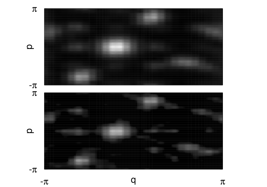
Figure 8: The local inverse participation ratio (LIPR) is plotted as a function of position and momentum for the potential of Eq. (32), with system size $N=64$, cusp location $q_{0}=-0.2\pi$, and cusp strength $v_{0}=0.59$. The exact LIPR landscape is shown in the upper panel, while the lower panel represents the prediction of a bootstrapping procedure with $T_{\rm max}=3$. The color scale ranges from LIPR=2 (black) to LIPR=5 (white).

V.2 Wave Function Intensity Distribution

A prescription similar to the above may be used to compute higher moments of the intensity distribution beyond the standard inverse participation ratio; instead, we turn our attention to the intensity distribution itself. Knowledge of such a distribution is essential, for example, to the understanding of resonance width or decay rate statistics in a weakly open system. In the context of scarring, it has been shown that the probability distribution of wave function intensities may be obtained by combining a smooth spectral envelope constructed from the short time dynamics with Gaussian random fluctuations on fine energy scales scarinten . More generally, whenever a separation of scales exists between non-random short-time dynamics and quasi-random long-time behavior, we may write the local density of states (strength function) for wave packet $\phi$ as papenbrock

$${\rm Re}\;(i/\pi)\,G_{\phi\phi}(E)=\sum_{n}\delta(E-E_{n})|\langle\phi|\Psi_{n}\rangle|^{2}\approx\sum_{n}\delta(E-E_{n})S^{\rm smooth}_{\phi}(E)|R_{n}|^{2}\,,$$ (33)

where

$$S^{\rm smooth}_{\phi}(E)=\sum_{\tau=-T}^{T}\langle\phi|\phi(t)\rangle e^{iEt/\hbar}$$ (34)

is a Fourier transform of the short-time signal and $R_{n}$ are independent Gaussian random variables with variance $1/N$ (real or complex depending on the presence or absence of time reversal symmetry, respectively). The above expressions assume no symmetry, with the possible exception of time reversal, and must be appropriately modified in the presence of such symmetries, including parity invariance scarmom . The multiplication in Eq. (33) of a known short-time signal by a long-time signal assumed to be quasi-random is the energy-domain counterpart of the convolution formula appearing in Eq. (28).

In the bootstrapping context, we may obtain the short-time envelope using Eqs. (9) and (10), where exact new recurrences ${\mathbf{B}}(m)$ are replaced by ${\mathbf{B}}_{L,\tau}(m)$ as defined by Eq. (11) for some choice of $T_{\rm max}=LT_{0}$ and a smoothing time scale $\tau$. This is the same procedure we used to construct approximate bootstrapped spectra in Sec. IV.2, except that there the bootstrap time $T_{\rm max}$ was chosen sufficiently long to resolve individual states, $T_{\rm max}>T_{H}/M$, while here we may take $T_{\rm max}$ to be only a small multiple of the one-step time $T_{0}$.

Once a short-time local density of states envelope $S^{\rm smooth}_{\phi}(E)$ is known, we may directly construct the probability distribution of wave function intensities $I=|\langle\phi|\Psi_{n}\rangle|^{2}$. We need only to multiply the envelope heights $S^{\rm smooth}_{\phi}(E)$, with uniformly distributed energies $E$, by random factors $|R|^{2}$ where $R$ is Gaussian-distributed (and $|R|^{2}$ is therefore exponentially distributed for complex $R$):

$$P(I)={1\over{E_{2}-E_{1}}}\int_{E_{1}}^{E_{2}}dE\int_{0}^{\infty}d(|R|^{2})e^{-|R|^{2}}\delta\left(I-S^{\rm smooth}_{\phi}(E)|R|^{2}\right)\,.$$ (35)

Typical examples of the resulting intensity distribution are shown in Fig. 9. Here we use the same system and wave packet location as in Fig. 7, but fix kick parameter $v_{0}$ at the value $0.2$. The short-time envelope $S^{\rm smooth}_{\phi}$ is constructed either using only one-step new recurrences (bootstrap time $T_{\rm max}=T_{0}=1$) or using one- and two-step new recurrences (bootstrap time $T_{\rm max}=2T_{0}=2$). The $T_{\rm max}=1$ short-time envelope already results in a predicted intensity distribution that is a great improvement over the RMT prediction, correctly predicting an excess of very large and very small wave function intensities at the cusp. The $T_{\rm max}=2$ envelope predicts an intensity distribution that is in even better agreement with actual data.

Figure 9: The distribution of wave function intensities $I=|\langle\phi|\Psi_{n}\rangle|^{2}$ for the kicked map of Eq. (32) with system size $N=64$, cusp location $q_{0}=-0.2\pi$, and kick parameter $v_{0}=0.2$ is shown, where $\phi$ is a Gaussian wave packet centered on the cusp at $q=q_{0}$, $p=0$. The solid curve shows the exact data, obtained by diagonalizing time evolution matrices, and averaging over systems with different boundary conditions. The bootstrapped predictions are computed using Eq. (35), where the smooth envelope is obtained from bootstrap time $T_{\rm max}=1$ or $T_{\rm max}=2$, for a single wave packet $M=1$. The RMT prediction, equivalent to bootstrapping with $T_{\rm max}=0$, provides a baseline for comparison.

V.3 Wave Function Correlations

The bootstrapping approach lends itself naturally to the consideration of observables beyond the statistics of individual wave function intensities $I=|\langle\phi|\Psi\rangle|^{2}$. As a simple example, we may consider the covariance ${\rm COV}_{\phi_{1},\phi_{2}}=N\sum_{j=1}^{N}|\langle\phi_{1}|\Psi_{j}\rangle|^{2}|\langle\phi_{2}|\Psi_{j}\rangle|^{2}-1$, where $\phi_{1}$ and $\phi_{2}$ are two wave packets and the sum is once again over the eigenstates. Obviously the covariance is a generalization to two wave packets of the local inverse participation ratio discussed earlier: ${\rm LIPR}_{\phi}={\rm COV}_{\phi,\phi}+1$. The covariance or correlation between wave function intensities at two points is clearly important, for example, for understanding the statistics of conductance peak heights in a weakly open quantum dot with two leads scarcond ; it is also relevant for analogous reaction rate calculations or for the computation of interaction matrix elements.

Letting $|\phi\rangle={1\over\sqrt{2}}(|\phi_{1}\rangle+e^{i\theta}|\phi_{2}\rangle)$, using Eq. (29) for ${\rm LIPR}_{\phi}$, and averaging over the relative phase $\theta$, we obtain

$${\rm COV}_{\phi_{1},\phi_{2}} \approx \sum_{\tau=-T}^{T}\left[|\langle\phi_{1}|\phi_{2}(\tau)\rangle|^{2}+\langle\phi_{1}|\phi_{1}(t)\rangle\langle\phi_{2}(t)|\phi_{2}\rangle\right]-1$$ (36)

$$= |C_{\phi_{1}\phi_{2}}(0)|^{2}+2\sum_{\tau=1}^{T}|C_{\phi_{1}\phi_{2}}(\tau)|^{2}+2\;{\rm Re}\sum_{\tau=1}^{T}C_{\phi_{1}\phi_{1}}(\tau)C^{\ast}_{\phi_{2}\phi_{2}}(\tau)$$

Two types of terms are present in Eq. (36): ones associated with the short-time probability for evolving from state $\phi_{1}$ to state $\phi_{2}$ or vice versa, and ones associated with a correlation between the individual short-time autocorrelation functions for $\phi_{1}$ and $\phi_{2}$. Once again, the correlation functions $C_{\phi\phi^{\prime}}(\tau)$ may be computed using the bootstrapping formula given by Eq. (7) or Eq. (8), where the “new” recurrences ${\mathbf{B}}(m)$ are known up to the bootstrap time $T_{\rm max}=LT_{0}$, as in Eq. (11). As in the LIPR calculation, the upper limit $T$ of the sum in Eq. (36) may be taken to infinity, as long as $T_{\rm max}<T_{H}/M$. For the covariance calculation, it is most convenient to perform the bootstrapping with just $M=2$ initial wave packets: $\phi_{1}$ and $\phi_{2}$.

As an example, we consider another quantum map, defined by Eq. (17) with kinetic term

$$T(p)={1\over 2}(p-p_{0})^{2}+b\left[\sin{2(p-p_{0})}-{1\over 2}\sin{4(p-p_{0})}\right]$$ (37)

and periodic kick

$$V(q)=\left\{\begin{array}[]{ll}-{a\over 2}(q+\pi/2)^{2}+v_{0}{q+\pi\over\pi/2}&-\pi<q<-\pi/2\\ -{a\over 2}(q+\pi/2)^{2}+v_{0}{q_{0}-q\over q_{0}+\pi/2}&-\pi/2<q<q_{0}\\ -{a\over 2}(q-\pi/2)^{2}+{3\over 2}v_{0}{q-q_{0}\over\pi/2-q_{0}}&q_{0}<q<\pi/2\\ -{a\over 2}(q-\pi/2)^{2}+{3\over 2}v_{0}{\pi-q\over\pi/2}&\pi/2<q<\pi\end{array}\right.$$ (38)

This potential has a cusp-like maximum of height $v_{0}$ at $q=-\pi/2$ and another of height $3v_{0}/2$ at $q=\pi/2$, resulting in the possibility of diffractive periodic motion between $(q=-\pi/2,p=p_{0})$ and $(q=\pi/2,p=p_{0})$. We compute the covariance between wave function intensities $|\langle\phi_{1}|\Psi\rangle|^{2}$ and $|\langle\phi_{2}|\Psi\rangle|^{2}$, where $\phi_{1}$ and $\phi_{2}$ are Gaussian wave packets centered at the two points in phase space. The results are presented in Fig. 10, as a function of the cusp height parameter $v_{0}$. Once again, the bootstrapping prediction is shown for bootstrap time $T_{\rm max}=1$ or $2$, in units where the kick period $T_{\rm kick}$ is set to unity. The RMT prediction, corresponding to bootstrap time $T_{\rm max}=0$, is shown for comparison. Just as in the LIPR and intensity distribution calculations, rapid convergence is observed with increasing $T_{\rm max}$, and almost all relevant information is already obtained by bootstrapping the one-step and two-step dynamics.

Figure 10: The covariance between wave function intensities $|\langle\phi_{1}|\Psi\rangle|^{2}$ and $|\langle\phi_{2}|\Psi\rangle|^{2}$, where $\phi_{1}$ and $\phi_{2}$ are Gaussian wave packets centered at $(q=\pm\pi/2,p=p_{0})$, is computed for a quantum map with kinetic term given by Eq. (37) and kick potential given by Eq. (38). Once again, the data is averaged over boundary conditions for each value of the kick parameter $v_{0}$. The system size is fixed at $N=256$, and the classical system parameters are $a=1/4$, $b=1/20$, $q_{0}=-\pi/5$ and $p_{0}=-3\pi/5$. The exact results of matrix diagonalization are compared with the bootstrapping calculation for $M=2$ wave packets with bootstrap time $T_{\rm max}=1$ or $2$, in units of the kick period.

VI Summary

Short-time dynamical information, either of classical origin or otherwise, inevitably leaves its imprint on the long-time behavior and stationary properties of a quantum system. The bootstrapping approach allows this information to be processed systematically, for one or an arbitrary number $M$ of initial wave packets. Because multiple iterations of the known short-time dynamics are included, the resulting spectral accuracy can be much greater than what one would obtain, for example, by a simple Fourier transform of a short-time signal. At the same time, the procedure is extremely efficient, requiring at each energy linear algebra operations involving only $M$ by $M$ matrices, and independent of the total size $N$ of the Hilbert space. There is no assumption of unitarity in the dynamics, and the procedure works equally well for closed or open systems. Robustness to errors in the short-time signal implies, for example, that reliable calculations can be performed when the short-time correlations are computed in a small-$\hbar$ or other approximation relevant to a given problem.

The bootstrap time $T_{\rm max}$ can be varied to extract maximum information from the least amount of input data. At small values of $T_{\rm max}$, the approach can be viewed as a generalization of standard periodic orbit scar theory, leading to statistical prediction beyond RMT for local density of states and wave function statistics. Reliable quantitative predictions can be obtained for inverse participation ratios, wave function intensity distributions, and wave function correlations, even when the short-time dynamics is of non-classical origin. Increasing either $T_{\rm max}$ or $M$ allows for a systematic inclusion of additional correlations. Once the product $MT_{\rm max}$ becomes comparable to the Heisenberg time $T_{H}$, it becomes possible to go beyond statistical predictions to resolve individual eigenstates and energy levels, with an accuracy scaling exponentially with $MT_{\rm max}/T_{H}$. The initial wave packets $\phi_{i}$ can be chosen optimally to minimize redundancy in the short-time correlations, and to obtain maximal information in a specific basis or for wave function structure in a given subspace of the original Hilbert space.

- (1) O. Bohigas, M.-J. Giannoni, and C. Schmit, J. Physique Lett. 45, L-1015 (1984); M. L. Mehta, Random Matrix Theory (Springer-Verlag, New York, 1990).
- (2) M. V. Berry, in Chaotic Behaviour of Deterministic Systems, edited by G. Iooss, R. Helleman, and R. Stora (North-Holland, 1983), p. 171; M. V. Berry, J. Phys. A 10, 2083 (1977); A. Voros, Ann. Inst. Henri Poincaré, Sect. A 24, 31 (1976).
- (3) E. J. Heller, Phys. Rev. Lett. 53, 1515 (1984); L. Kaplan and E. J. Heller, Annals of Physics 264, 171 (1998).
- (4) W. E. Bies, L. Kaplan, M. R. Haggerty, and E. J. Heller, Phys. Rev. E 63, 066214 (2001).
- (5) S. Sridhar and W. T. Lu, J. Stat. Phys. 108, 755 (2002); N. B. Rex, H. E. Tureci, H. G. L. Schwefel, R. K. Chang, and A. D. Stone Phys. Rev. Lett. 88, 094102 (2002); O. Agam and B. L. Altshuler, Physica A 302, 310 (2001); S. C. Creagh, S.-Y. Lee and N. D. Whelan, Annals of Physics (N.Y.) 295, 194 (2002).
- (6) P. B. Wilkinson, T. M. Fromhold, L. Eaves, F. W. Sheard, N. Miura, and T. Takamasu, Nature 380, 608 (1996); E. E. Narimanov and A. D. Stone, Phys. Rev. Lett. 80, 49 (1998).
- (7) E. E. Narimanov, N. R. Cerruti, H. U. Baranger, and S. Tomsovic, Phys. Rev. Lett. 83, 2640 (1999).
- (8) J. S. Hersch, M. R. Haggerty, and E. J. Heller, Phys. Rev. E 62, 4873 (2000); see also S.-Y. Lee, S. Rim, J.-W. Ryu, T.-Y. Kwon, M. Choi, and C.-M. Kim, Phys. Rev. Lett. 93, 164102 (2004).
- (9) L. Kaplan and T. Papenbrock, Phys. Rev. Lett. 84, 4553 (2000).
- (10) G. Berkolaiko, J. P. Keating, and B. Winn, Phys. Rev. Lett. 91, 134103 (2003); H. Schanz and T. Kottos, ibid. 90, 234101 (2003); L. Kaplan, Phys. Rev. E 64, 036225 (2001).
- (11) E. Bogomolny and C. Schmit, Phys. Rev. Lett. 92, 244102 (2004); L. Kaplan and E. J. Heller, Physica D 121, 1 (1998).
- (12) H. Schanz, arXiv:nlin.CD/0409055 (unpublished); S. Hortikar and M. Srednicki, Phys. Rev. Lett. 80, 1646 (1998).
- (13) V. A. Mandelshtam, Prog. Nucl. Magn. Reson. Spectrosc. 38, 159 (2001); J. Main, V. A. Mandelshtam, and H. S. Taylor, Phys. Rev. Lett. 79, 825 (1997); M. R. Wall and D. Neuhauser, J. Chem. Phys. 102, 8011 (1995).
- (14) E. B. Bogomolny, Nonlinearity 5, 805 (1992).
- (15) S. Fishman, D. R. Grempel, and R. E. Prange, Phys. Rev. Lett. 49, 509 (1984); A. Altland and M. R. Zirnbauer, ibid. 77, 4536 (1996).
- (16) P. A. Boasman and J. P. Keating, Proc. R. Soc. London, Ser. A 449, 629 (1995).
- (17) B. Barbanis, Aston. J. 71, 415 (1966).
- (18) D. V. Savin and V. V. Sokolov, Phys. Rev. E 56, R4911 (1997); H.-J. Sommers, D. V. Savin, and V. V. Sokolov, Phys. Rev. Lett. 87, 094101 (2001); P. W. Brouwer, K. M. Frahm, and C. W. J. Beenakker, ibid. 78, 4737 (1997).
- (19) L. Kaplan and E. J. Heller, Phys. Rev. E 59, 6609 (1999).
- (20) A. D. Mirlin and F. Evers, Phys. Rev. B 62, 7920 (2000); A. Wobst, G.-L. Ingold, P. Hanggi, and D. Weinmann, ibid. 68, 085103 (2003).
- (21) L. Kaplan, Phys. Rev. Lett. 80, 2582 (1998).