DYNAMICS OF THREE VORTICES
ON A PLANE AND A SPHERE — II.
General compact case

A. V. BORISOV
Faculty of Mechanics and Mathematics
Department of Theoretical Mechanics Moscow State University
Vorob’ievy gory, 119899 Moscow, Russia
E-mail: borisov@uni.udm.ru
V. G. LEBEDEV
Physical Faculty,
Department of Theoretical Physics Udmurt State University
Universitetskaya, 1, Izhevsk, Russia, 426034
E-mail: lvg@uni.udm.ru

Abstract

Integrable problem of three vortices on a plane and sphere are considered. The classification of Poisson structures is carried out. We accomplish the bifurcational analysis using the variables introduced in previous part of the work.

1 Introduction

In this part of our work the integrable problem of dynamic of vortices on planes and sphere are considered. We base on Hamiltonian form of reduced systems, which poisson structure was given in the previous part [18].

The problem of motion of two vortices on plane was completely investigated by G. Helmholz [14], who had established, that in general case two vortices make an uniform rotary motion around of vorticity centre, with frequency

$$\Omega=\frac{\Gamma_{1}+\Gamma_{2}}{2\pi r^{2}},$$

where $\Gamma_{k}$ is intensity of point vortices. The vorticity centre thus is moving uniformly and rectilinearly. If $\Gamma_{1}=-\Gamma_{2}$ the vorticity centre is situated on infinity, and two vortices are moving forward.

The problem about a motion of three vortices is much more complex. Despite of numerous works, first of which were the dissertation of  Gröbli 1877 [2] and Greenhill’s research [5], the complete and evident classification of a motion still does not exist. From the point of view of integrability problem, this problem was considered by Poincare in the treatise on the vortices theory [3]. He wrote out explicitly a complete set of noncommutative integrals. In a modern period the problem of a motion of three vortices on a plane was studied in works [12, 10, 13, 19, 20], and from the point of view of the topological analysis — in [15]. Unfortunately, these works have added a little to achievements of classicists both in presentation, and in completeness of the description of motions. Their basic contents come down either to geometrical interpretation of a motion and computer modeling of separate trajectories, or to some general topological constractions, that is not coordinated to physical behaviour of system. Partly, it is caused by the fact, that the problem of three vortices on a plane does not belong to that integrable systems, which complete analysis is possible in a class of rather simple (for example, elliptic) special functions (the general solution has indefinitely–sheeted branching on complex plane of time because of logarithmic terms in Hamiltonian). The exception consists of some special cases (for example, the case of equal intensities of vortices). In comparison with a problem of three vortices on a plane, a motion of three vortices on sphere, that is also being integrable, is not investigated at all.

We give here new analysis, based on algebraic and geometrical research of the reduced system (in variable, which in the previous part of work [18] were named “internal”, as though we are not adhere this term anymore), and then we analyze absolute motion, without use of exact quadrature. Such approach, basing on representation of the equations of motions on algebra [18], allows to establish some analogies between problem of three vortices and Euler-Poinsot case in rigid body dynamics, and also to receive more evident description of motions of system.

2 Algebraic classification

As it was shown in the previous part of work [18], the equation of a motion of three vortices on the plane can be written down as Hamiltonian system, determined by Lie-Poisson brackets in form of

$$\begin{array}[]{l}\displaystyle\{M_{i},M_{j}\}=-4a_{k}\Delta,\vskip 6.0pt plus 2.0pt minus 2.0pt\\ \displaystyle\{M_{i},\Delta\}=(a_{j}-a_{k})M_{i}+(a_{j}+a_{k})(M_{j}-M_{k}),\\ \end{array}$$ (1)

and by Hamiltonian

$$H=-{1\over 8\pi}(\Gamma_{2}\Gamma_{3}\log M_{1}+\Gamma_{1}\Gamma_{3}\log M_{2}+\Gamma_{1}\Gamma_{2}\log M_{3}).$$ (2)

where $M_{k}$ are squares of pairwise distances between vortices, $\Delta$ is a size of the oriented area pulled on three vortices (here and further we shall assume, that the indexes $i,j,k$ accept accordingly values $1,2,3$ and their cyclic rearrangements, and the coefficients $a_{1},a_{2},a_{3}$ are inverse intensities $a_{k}=1/{\Gamma_{k}}).$

Lie-Poisson brackets (1) are degenerated and have two central functions. One of them (linear) is integral of the complete moment

$$D=\sum_{k}a_{k}M_{k},$$ (3)

the other (square-law Casimir function) arises from geometrical Henon ratio, that connects the area of triangle with sides

$$F=(2\Delta)^{2}+M_{1}M_{1}+M_{2}M_{2}+M_{3}M_{3}-2(M_{1}M_{2}+M_{1}M_{3}+M_{2}M_{3}).$$ (4)

For real motions $F=0.$

The real type of Lie-Poisson algebra (1) depends on values of intensities $\Gamma_{1},\Gamma_{2},\Gamma_{3}.$ In fact, choosing a new basis in form $D,e_{1},e_{2},e_{3}$, where $D$ is defined by (3)

$$\begin{array}[]{l}\displaystyle e_{1}=\frac{\Delta}{2\sqrt{A}},\\ \displaystyle e_{2}=\frac{(a_{2}-a_{3})M_{1}+(a_{3}-a_{1})M_{2}+(a_{1}-a_{2})M_{3}}{2\sqrt{2AB}},\\ \displaystyle e_{3}=\frac{(a_{2}a_{3}-a_{1}^{2})M_{1}+(a_{1}a_{3}-a_{2}^{2})M_{2}+(a_{1}a_{2}-a_{3}^{2})M_{3}}{2A\sqrt{2B}}\\ \end{array}$$ (5)

where

$$A=|a_{1}a_{2}+a_{2}a_{3}+a_{1}a_{3}|,$$

$$B=(a_{1}-a_{2})^{2}+(a_{2}-a_{3})^{2}+(a_{1}-a_{3})^{2},$$

under the condition

$$(a_{1}a_{2}+a_{2}a_{3}+a_{1}a_{3})>0,$$ (6)

we receive that the algebra of vortices is decomposed in the direct sum $l(4)\approx$ $\mathbb{R}\oplus so(3):$

$$\{D,e_{k}\}=0\mbox{, }\{e_{1},e_{2}\}=e_{3}\mbox{, }\{e_{2},e_{3}\}=e_{1}\mbox{ }\{e_{3},e_{1}\}=e_{2},$$ (7)

and by condition

$$(a_{1}a_{2}+a_{2}a_{3}+a_{1}a_{3})<0,$$ (8)

in direct sum $l(4)\approx$ $\mathbb{R}\oplus so(2,1):$

$$\{D,e_{k}\}=0,\quad\{e_{1},e_{2}\}=-e_{3},\quad\{e_{2},e_{3}\}=e_{1},\quad\{e_{3},e_{1}\}=e_{2}.$$ (9)

Though for case equal intensities the coefficient $B=0$, using the passage to the limit, it is easy to show that basis (5) can be correctly determined in this case as well.

Let’s consider, what features of a motion can be obtained from the structure of such algebraic decomposition. Using squared Casimir function for algebra $so(3)$

$$G^{2}=e_{1}^{2}+e_{2}^{2}+e_{3}^{2},$$ (10)

and expressing in it a vector $e_{1}$ with the help of Heron ratio (4) with $F=0,$ we discover, that relative dynamics of vortices with intensities, satisfying to a condition (6) will be equivalent to a motion of some ”representing” point on symplectic sheet, that is a two-dimensional sphere with radius, determined by value of linear Casimir function

$$e_{1}^{2}+e_{2}^{2}+e_{3}^{2}=\frac{1}{16}\left(\frac{a_{1}a_{2}a_{3}D}{a_{1}a_{2}+a_{2}a_{3}+a_{1}a_{3}}\right)^{2}.$$ (11)

The situation for algebra $so(2,1)$ is similar that arise in a case (8). Using Casimir function of algebra $so(2,1)$

$$G^{2}=e_{3}^{2}-e_{2}^{2}-e_{2}^{2},$$ (12)

it is possible to notice, that the relative motion of vortices is reduced to the motion of point on surface of two-cavities hyperboloid, that is determined by condition,

$$e_{3}^{2}-e_{1}^{2}-e_{2}^{2}=\frac{1}{16}\left(\frac{a_{1}a_{2}a_{3}D}{a_{1}a_{2}+a_{2}a_{3}+a_{1}a_{3}}\right)^{2}.$$ (13)

In case of (6), motions of representing point (and therefore three vortices in system of vorticity centre) is finite for every $D$, therefore this case we shall futher name “compact”, and in case (8), with which obviously may be exist running up trajectories by additional conditions for $\Gamma_{i}$ and for initial vortices positions, the name “uncompact”.

Motions, arising under condition

$$(a_{1}a_{2}+a_{2}a_{3}+a_{1}a_{3})=0$$ (14)

require separate consideration. In basis

$$\begin{array}[]{l}\displaystyle D=\frac{a_{1}M_{1}+a_{2}M_{2}+a_{3}M_{3}}{(a_{1}+a_{2})^{2}},\\ \displaystyle e_{1}=\frac{\Delta}{(a_{1}+a_{2})},\\ \displaystyle e_{2}=\frac{M_{3}}{2(a_{1}+a_{2})},\\ \displaystyle e_{3}=\frac{(a_{1}+a_{2}+a_{3})M_{3}-(M_{1}+M_{2})(a_{1}+a_{2})}{2(a_{1}+a_{2})^{2}},\\ \end{array}$$ (15)

Lie-Poisson brackets can be reduced to form

$$\{D,e_{k}\}=0,\quad\displaystyle\{e_{1},e_{2}\}=e_{3},\quad\displaystyle\{e_{3},e_{1}\}=-D,\quad\displaystyle\{e_{2},e_{3}\}=e_{1}.$$ (16)

In this case algebra of vortices is not decomposed in the straight sum of one-dimensional and three-dimensional algebras, and becomes four-dimensional solveable algebra with maximal solveable ideal $N=\{D,e_{1},e_{3}\}.$ Algebra has squared Casimir function, following from (4)

$$G^{2}=e_{1}^{2}+e_{3}^{2}-2De_{2}.$$ (17)

Real dynamics of vortices occurs on symplectic sheet, that is set by conditions $G=0$ and $D~{}=~{}const,$ which determine paraboloid, taking place through the beginning of coordinates. By $D=0$, being necessary collaps condition (merge of vortices), paraboloid degenerates to the straight line, conterminous with an axis $e_{3}.$

3 Bifurcational analysis of motion of vortices on plane

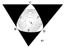
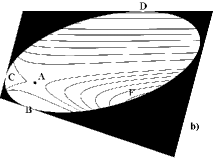
Figure 1: Dark part corresponds to nonphysical area on a plane, that is set by linear integral $D=const$ and limited by conditions $M_{k}>0,$ for a compact case: a) All of intensities are positive; b) One of intensities is negative. The point $A$ corresponds to the Tomson’s solution; $F$ — collilear solutions; $B,C,D$ — points, in with which two vortices are merged in one.

Let’s describe most evident geometrical interpretation of motions, used in [19] and presented on Fig. 1. In space $M_{1},M_{2},M_{3}$ the level of linear integral of the moment sets a plane. The inequalities $M_{k}>0$ allocate on it the area, in which motion occurs. It is necessary to exclude from this area unphysical values of distances, for which an inequality of a triangle $(\Delta^{2}<0)$ does not hold. This area is shown at a figure by black colour. When approaching to it, in the equations of a motion for variable $M_{1},M_{2},M_{3},$ we schould change the sign of time and direction of motion. It is necessary to note, that the described geometrical interpretation is not equivalent to a motion of representing point on symplectic sheet, and changes of direction of motions are the consequence of features of a projection from space $\Delta,M_{1},M_{2},M_{3}$ in space $M_{1},M_{2},M_{3}.$

Let’s hold condition (6), then bracket (1) is defines algebra $so(3)\oplus\mathbb{R}$. In this case symplectic sheet is compact ($\mathbb{S}^{2}$), and motions of vortices are finite. Let’s assume, at first, that signs of all intensities are identical — in this case condition (6) is obviously fullfiled. The first integrals of a motion of vortices on a plane we shall write down as

$$\begin{array}[]{l}\displaystyle D=a_{1}M_{1}+a_{2}M_{2}+a_{3}M_{3},\vskip 6.0pt plus 2.0pt minus 2.0pt\\ \displaystyle h=M_{1}^{a_{1}}M_{2}^{a_{2}}M_{3}^{a_{3}},\\ \end{array}$$ (18)

(integral of energy, for convenience, is presented in exponential form). The integrals (18) are dependent, i.e. Jacobi matrix of the first integrals (18) is degenerate

$$Rank\left(\frac{\partial(D,h)}{\partial(M_{1},M_{2},M_{3})}\right)<2$$ (19)

only in one case: $M_{1}=M_{2}=M_{3}$ (in three-dimensional space $M_{1},M_{2},M_{3}$ the vortices will form correct triangle). Curves, resulting with crossing of levels of integrals (18) are similar to polhodes in rigid body dynamics (Poinsot interpretation of Euler case) and, in a compact case, are ovals (Fig. 1). The solution as correct triangle occurs with a contact of a surface $h$ and plane $D$ in one point. They limit by energy the area of possible motions (APM) from above and the corresponding bifurcational curve has a form

$$H(D)=\left(\frac{D}{\sum a_{i}}\right)^{(\sum a_{i})}.$$ (20)

Remark 1. The particular solutions, appropriate to the given curve — three vortices in tops of correct triangle, rotating as a rigid body around of vorticity centre are refered as “Thomson’s” and are steady with fulfilment of a condition (6). J. J. Thomson has specified them for any number of vortices of equal intensity, and has shown, that in linear approach such configurations will be steady for number of vortices $N\leqslant 6$, and with $N\geqslant 7$ — unstable (Thomson theorem) [1]. However because of presence of resonances in system the linear approach is not sufficient. The analysis of stability in nonlinear approach with use of Birkhoff normalization was carried out in [6]. It was found, that the theorem Thomson is fair in the exact statement — in sense of Laypunov stability.

The other change of motion occurs with a contact of a crossing line of integrals’ levels with curves, determined by the equation $\Delta(M_{1},M_{2},M_{3})=0$ $(\sqrt{M_{i}}+\sqrt{M_{j}}=\sqrt{M_{k}}),$ that arise from inequalities of triangles and limit physically allowable area of values (see Fig. 1).

Points of a contact correspond to collinear configuration of three vortices. Three vortices thus settle down on one straight line and rotate as a unit around of vorticity centre.

Remark 2. Collinear and the triangular configurations in dynamics of three vortices have analogues in the classical selestial mechanics [11]. There are, accordingly, Euler and Lagrange particular solutions of three body problem.

Collinear configurations are obtained from a condition of a contact

$$\Delta=0,\quad\dot{\Delta}=0.$$ (21)

that lead, having same sedate functional dependence, which in a general case can be presented as

$$H(D)=f(a_{1},a_{2},a_{3})D^{(a_{1}+a_{2}+a_{3})},$$ (22)

where $f(a_{1},a_{2},a_{3})$ some function from parameters. Passing to homogeneous coordinates $x,y$

$$M_{1}=xM_{3},\quad M_{2}=yM_{3},\quad y=(1+x)^{2},\quad x=z^{2},$$ (23)

we discover, that collinear configurations correspond to positive roots of the equations of the third degree

$$\alpha_{1}(1\pm z)(z\pm 2)+\alpha_{2}((1\mp z)z-\alpha_{3}(1\pm 2z)z(1\pm z)=0,$$ (24)

where

$$\alpha_{1}={\Gamma_{2}+\Gamma_{3}},\quad\alpha_{2}={\Gamma_{1}+\Gamma_{3}},\quad\alpha_{3}={\Gamma_{1}+\Gamma_{2}}.$$

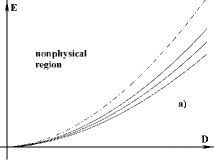
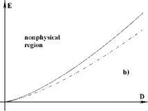
Figure 2: The view of bifurcation diagram for three vortices on a plane in compact case: a) With positive intensities; b) One negative intensity. The dot-dashed line corresponds to the Thomson’s solution, continuous lines — to collinear configurations.

The lines of crossing of levels $D$ and $h$ can concern borders of area of physically possible motion $\Delta=0$ in space of variables $(M_{1},M_{2},M_{3})$ by various ways (Fig. 1). Depending on it the quantity of bifurcational curves also will be different. In particular, in a case, when all of intensities are different $a_{1}\neq a_{2}\neq a_{3}\neq a_{1}$ three branches corresponding to collinear motions will exist (Fig. 2a). With equality of two of them, for example, $a_{1}=a_{2}\neq a_{3}$ two appropriate bifurcational curves merge. And, at last, in case of equal intensities $a_{1}=a_{2}=a_{3}$ all three curves degenerate in one.

The calculation of angular speed of Thomson’s and collinear configurations concerning vorticity centre is given, for example in [14]. It monotonously decreases with increase of the complete moment of system vortices.

As a measure of stability of stationary configurations it is possible to use a square of untrivial eigenvalues $\lambda^{2}$ of linearized system of the equations of a motion of three vortices. For Thomson’s configurations it is simple to receive the explicit formula

$$\lambda^{2}=-3a_{1}a_{2}a_{3}\frac{(a_{1}+a_{2}+a_{3})^{3}}{D^{2}},$$ (25)

that shows, that in a considered case they are steady, in difference from collinear, which as shown on Fig. 2a a are unstable.

Generally speaking, the following statement is fair, that is confirmed by geometrical interpretation on Fig. 1: If Thomson’s solution is steady, the appropriate set of collinear solutions are unstable, and on the contrary. Therefore condition (25) determines a type of stability not only Thomson’s configurations, but also collinear configurations with the given values of $D.$

Let’s consider other case of a motion of three vortices, with fullfiled conditions (6) (easy to see, that all other possible cases, when the condition is fair, could be reduced to two considered cases). Let’s assume, that the intensity of one of vortices has opposite sign in comparison with other two (for example, $\Gamma_{1}=1/a_{1}<0$). The condition (6) in this case means, that $-\Gamma_{1}<\Gamma_{2}+\Gamma_{3}$ (i.e. intensity of chosen vortex is greater than the intensity of other two).

Let’s specify only main differences of this problem from previous. First of all from the formula (25) for Thomson’s configurations it follows, that they are unstable. Collinear configuration (it is not three of them anymore, but only one) thus, on the contrary, is steady. Bifurcational curve of appropriate unique collinear configuration (see Fig. 2b) is above a curve, appropriate to Thomson’s configuration (it is simple to show, that under condition of (6) complete moment is always more than zero), and the area of possible motion coincides with the whole square $D>0,\quad h>0$.

To obtain more complete representation about the considered motions, let’s study a phase portrait of system of three vortices on a plane in symplectic coordinates.

4 Symplectic coordinates for vortices on a plane

Since symplectic sheets represent two-dimensional spheres (18), it is convenient to use cylindrical coordinates $l,L$ as canonical coordinates (we shall keep for them a designation of Andoyer–Deprit coordinates, adopted in rigid body dynamics [16]) for algebra $so(3):$

$$\begin{array}[]{l}\displaystyle e_{1}=L,\\ \displaystyle e_{2}=\sqrt{G^{2}-L^{2}}\sin l,\\ \displaystyle e_{3}=\sqrt{G^{2}-L^{2}}\cos l.\\ \end{array}$$ (26)

Expressions for variables $M_{1},M_{2},M_{3}$ in canonical coordinates look like

$$\begin{array}[]{ll}M_{i}=&\frac{\displaystyle a_{j}+a_{k}}{\displaystyle\sqrt{2}}{\displaystyle\frac{D}{A}}+2F(a_{j}-a_{k})F\sqrt{\frac{\displaystyle A}{\displaystyle B}}\sin l+\vskip 6.0pt plus 2.0pt minus 2.0pt\\ &{\displaystyle\frac{4F}{\sqrt{B}}}(a_{j}(a_{j}-a_{i})+a_{k}(a_{k}-a_{i}))\sqrt{\frac{2}{B}}\cos l,\\ \end{array}$$ (27)

where

$$A=a_{1}a_{2}+a_{2}a_{3}+a_{3}a_{1},$$

$$B=(a_{1}-a_{2})^{2}+(a_{2}-a_{3})^{2}+(a_{1}-a_{3})^{2},$$

$$F=\sqrt{G^{2}-L^{2}}.$$

In that special case of equal intensities the derived expressions (12) lead to the expression for Hamiltonian mentioned in [12, 21]. In last work it is used the classical way of a reduction to a problem with one degree of freedom for arbitrary intensities (such as Jacobi’s unit elimination).

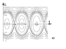
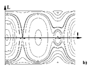
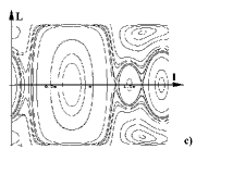
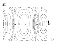
Figure 4: Phase plane for cases: a) Positive equal intensities; b) Case $a_{1}=a_{2}\neq a_{3}$ c) Three positive various intensities; d) One negative intensity.

The phase portrait in canonical coordinates describes a motion of representing point $(L,l)$ on a surface of two-dimensional sphere. The pulse $L$ has a value of the oriental area parallelogram, that is constructed on three vortices $(L=2\Delta)$. Development of a phase portrait is presented on Fig. 4a–d for four different specific cases of the intensities of vortices ratio.

The given figures illustrate the analogy between the motion of three vortices and rigid body dynamics. Comparing Fig. 2a (in case of equal intensities) with phase portrait of a Euler-Poinsot problem (see for example [16]), it is possible to connect a collinear configuration (situated on a straight line $L=0$) with unstable permanent motions of a rigid body around of an middle axis of ellipsoid of inertia, the Thomson’s solutions (with $L/G=1$) — with rotations around of a large (small) axis of ellipsoid of inertia. The periodic solutions of a problem of two vortices (two of three vortices always are in one point, and their intensities are added), situated on straight line $L=0$ it is possible to connect with steady permanent rotations around of a small (large) axis of elipsoid of inertia. When system pass through the collinear state ( three vortices on one straight line — $L=0$), oriented area changes the sign. Deformation of a phase picture with unequal intensities is shown on Fig. 4b,c. Thus Thomson’s solutions are displaced with straight $L/G=1,$ that on sphere should be imagined as being pulled together in a point). Fig. 4d present the phase portrait, with one negative intensity, but condition (6) is also fullfiled.

Other motions of system of three vortices, that is not a state of equilibrium on phase portraits, correspond to quasiperiodic motions of vortices on a plane. Depending on the topology of a phase curve these motions have various features — some of them repeatedly pass through the collinear state, others — never get into it. Such areas are separated by separatrix curve, for that curve three vortices are approach to collinear (unstable) configuration infinitely long. The particular trajectories of vortices are given in various works [10, 12, 13, 14, 19], beginning from Gröbli [2] and Greenhill [5].

Appropriate simplectic coordinates for algebra $so(2,1)$ could be chosen as

$$\begin{array}[]{l}\displaystyle e_{1}=L,\\ \displaystyle e_{2}=\sqrt{G^{2}+L^{2}}\mbox{\, sh}\,l,\\ \displaystyle e_{3}=\sqrt{G^{2}+L^{2}}\mbox{\, ch}\,l.\\ \end{array}$$ (28)

where $G,$ as well as in a case $so(3)$, parametrize various simplectic sheets. The difference of the case (8) is displayed in noncompactness of symplectic sheet, therefore the leaving of vortices to infinity is possible, that is excluded for condition (6).

5 Three vortices on sphere

The problem of motion of vortices on sphere is more interesting, but less investigated. This problem has more important applied meaning in comparison with a problem of motion of vortices on a plane, because it is directly connected with physics of atmosphere. Many substantial problems (collapse and evasion of vortices, existence of steady stationary (static) configurations) can be investigated on model of an ideal liquid. Their solutions can become a basis for more complex models (connected, for example, with presence of small viscosity), that describe real dynamic vortical processes (motion of cyclones and etc.) in an atmosphere of the Earth.

Dynamics of two vortices on sphere is quite similar to a flat case. Here the general situation is the rotation around of an axis, that is passing through centre of spheres and analogue of vorticity centre (point located on chord, connecting two vorteces with radius-vector

$$\vec{r}=\frac{\Gamma_{1}\vec{r}_{1}+\Gamma_{2}\vec{r}_{2}}{\Gamma_{1}+\Gamma_{2}},$$

where $\vec{r}_{1},\vec{r}_{2}$ — radius-vector of the first and second vortices). As well as in a flat case distance between vortices remains constant. Angular speed of such rotation

$$\Omega=\frac{1}{2\pi M}\sqrt{(\Gamma_{1}+\Gamma_{2})^{2}-\frac{\Gamma_{1}\Gamma_{2}M}{R^{2}}},$$ (29)

where $R$ — radius of sphere, $M$ — square of distance between the vortices (square of the length of a chord, that connect the location of two vortices on sphere). Under condition of $\Gamma_{1}=-\Gamma_{2}$, two vortices are moving on sphere on two identical parallels, located on different parties from equator, that was noticed Gromeka [4].

The problem of motion of three vortices on sphere was considered in work [9], in that work probably for the first time the integrability of the problem was specified. The equations of motion of three vortices on sphere in variables of mutual distances (chords) and volumes can be written down [18] as the Hamiltonian equations with nonlinear algebra of Poisson brackets

$$\begin{array}[]{l}\displaystyle\{M_{i},M_{j}\}=-\frac{4a_{k}\Delta}{R},\\ \displaystyle\{M_{i},\Delta\}=R(a_{j}-a_{k})M_{i}+R(a_{j}+a_{k})(M_{j}-M_{k})+\frac{M_{i}}{2R}(a_{k}M_{k}-a_{j}M_{j}),\\ \end{array}$$ (30)

that also have two central functions, one of them (linear) is the same as (3), and the second (cubic) function has the form

$$\begin{array}[]{rl}F=&(2\Delta)^{2}+R^{2}(M_{1}M_{1}+M_{2}M_{2}+M_{3}M_{3})-2R^{2}(M_{1}M_{2}+\vskip 6.0pt plus 2.0pt minus 2.0pt\\ &M_{1}M_{3}+M_{2}M_{3})+M_{1}M_{2}M_{3}=0,\end{array}$$ (31)

and Hamiltonian (2).

Let’s notice, that linear approximation of structure (30) coincides with the Poisson bracket of three vortices on a plane. Besides, it is simple to show, that after replacement

$$\frac{d\tau}{dt}=\pm\frac{\Delta}{2\pi M_{1}M_{2}M_{3}}$$

the equations of a motion of vortices turn in Lotky–Volterra system of the form

$$\frac{d}{d\tau}M_{i}=\Gamma_{i}M_{i}(M_{j}-M_{k}),$$ (32)

similarly to the flat case [18]. This trajectory isomorphism is also piecewise [18].

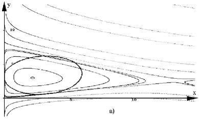
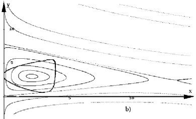
Figure 7: Geometrical picture is isomorfic with a Lotky-Volterra problem. A part of a phase plane of Lotky-Volterra, that is limited by a contour, corresponds to physical area of a problem of three vortices: a) on a plane; b) on sphere with a set of identical intensities.

Geometrical interpretation for a plane, presented on Fig. 1, can be also transferred to sphere. Curious and earlier, probably, not marked fact is that phase trajectories in variable $M_{1},M_{2},M_{3}$ for a case of sphere and plane, with given intensities, coincide with phase trajectories of the same Lotky–Volterra system (30). Thus main effects in dynamics of vortices are determined by the part of phase trajectories of Lotky–Volterra system gets that in area $\Delta^{2}(M_{1},M_{2},M_{3})>0.$ The motion of vortices occurs only in this part, because with the approach of trajectories to border of area (and achievement by vortices collinear state) in the equations (32) it is necessary to change a sign of time. The form of this area is a little various for a plane and sphere (formula (4) and (31)) and represented on Fig. 7.

Remark 3. The analogy with Lotky–Volterra system is very useful for study of vortices collaps problem and is related to Bolin regularization in the [11] (the difference is, that in the Kepler problem is fixed a constant of energy level). Problems of regularization and collapse, that arise only in noncompact cases, will be discussed in the next part of work.

Remark 4. The issue of reduction of three vortices problem on sphere to canonical Hamiltonian system with one degree of freedom is complex and, probably, it could not be solved constructively. If one use the initial form of record [18], then one obtain the six-dimensional Hamiltonian system, that have as the integrals Hamiltonian function and noncommutative set of integrals of moment, each of them is nonlinear function of phase variable (in difference from a case of a plane considered in [21]).

The canonization of the reduced system also problematic, in variable $(\vec{M},\Delta)$ the canonization is equivalent to introduction of Darboux coordinates on two-dimensional symplectic sheet determined by a common level of Casimir functions. It require the the solution of nonlinear system of the partial differential equations.

Really, the nonlinear algebra of Poisson brackets (30) cannot be investigated in same detail, as in the flat case. Linear approximation of this structure is capable to make some qualitative conclusions only for a situation close to simultaneous collaps (i.e. when distance between vortices is small in relation to radius of curvature). From it, nevertheless, it is possible to make a conclusion that necessary conditions of simultaneous collaps of vortices on a plane are also fair for the case of sphere, since the influence of nonlinear terms is small enough near the collaps.

The most simple form the bracket (30) has in case of three equal intensities at a zero level of linear Casimir function $(D=0).$ After transition (for linearization of a bracket (30)) to canonical basis (5) it is possible to present bracket

$$\begin{array}[]{l}\displaystyle\{e_{1},e_{2}\}=e_{3}+\frac{1}{2}(e_{3}^{2}-e_{2}^{2}),\\ \displaystyle\{e_{2},e_{3}\}=e_{1},\\ \displaystyle\{e_{3},e_{1}\}=e_{2}-e_{2}e_{3}.\\ \end{array}$$ (33)

It is curious to note, that nonlinear terms, included in a bracket, (33), are similar to the terms, originating in Kovalevsky integral of the Euler–Poisson equations [18].

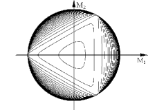
Figure 5: Deformation of section of symplectic sheet for linearized algebra of vortices on sphere depending on change of sphere’s radius of curvature.

One of main sections of sheet for a case $\Gamma_{1}=\Gamma_{2}=\Gamma_{3}$ are shown on Fig. 5 in dependence from curvature of sphere $k=1/R$. With $k=0,$ the symplectic sheet, that is determined by algebra $So(3)$, is also sphere. The change $k$ results in a surface, whose coherent component is homeomorphic to sphere. It would be interesting to investigate the topology of a symplectic sheet with various values of intensities and values of integral of the moment $D$, that is the limited function on sphere (on which vortices move). Last remark allows to reject uncompact components of symplectic sheets, since a motion on sphere is always finite.

Remark 5. The general principle of the classification of vortices motions on sphere given below is the continuation on parameter of complete moment of stationary configurations that is known near $D=0.$ In last case the influence of curvature is not significant, that corresponds already investigated flat problem (it is also equivalent to consideration of linear approximation of structure (30)).

The conditions for Thomson’s of configurations on sphere are similar to conditions on plane

$$M_{1}=M_{2}=M_{3}.$$

Conditions for existence of collinear configurations $(\Delta=\dot{\Delta}=0)$ in case of sphere are reduced to system of three algebraic equations. Introducing constants

$$\alpha_{1}=\Gamma_{3}+\Gamma_{2},\quad\alpha_{2}=\Gamma_{1}+\Gamma_{3},\quad\alpha_{3}=\Gamma_{2}+\Gamma_{1},\quad\beta_{1}=\Gamma_{3}-\Gamma_{2},\quad\beta_{2}=\Gamma_{1}-\Gamma_{3},\quad\beta_{3}=\Gamma_{2}-\Gamma_{1},$$

we write down system of the equations as

$$\begin{array}[]{l}\displaystyle 2(M_{1}M_{2}+M_{1}M_{3}+M_{2}M_{3})-(M_{1}^{2}+M_{2}^{2}+M_{3}^{2})-\frac{M_{1}M_{2}M_{3}}{R^{2}}=0,\\[12.0pt] \displaystyle a_{1}M_{1}+a_{2}M_{2}+a_{3}M_{3}-D=0,\\[12.0pt] \displaystyle 2(\alpha_{1}\frac{(M_{3}-M_{2})}{M_{1}}+\alpha_{2}\frac{(M_{1}-M_{3})}{M_{2}}+\alpha_{3}\frac{(M_{2}-M_{1})}{M_{3}}+\\[12.0pt] \displaystyle(\beta_{1}M_{1}+\beta_{2}M_{2}+\beta_{3}M_{3})\frac{1}{R^{2}}=0,\\[12.0pt] \end{array}$$ (34)

where $D$ is the value of integral of the moment. The given system can be solved numerically. Results of numerical research of bifurcational diagrams for cases of various values of intensities are presented on Fig. 6.

Remark 6. As well as in case of a plane we are interesting only in positive roots of the equations (34). Besides we should notice, that range of values of functions, determined by integrals of energy and moment are limited by values $D_{m}$ and $E_{m}$

$$D_{m}=4R^{2}\frac{(a_{1}a_{2}+a_{2}a_{3}+a_{1}a_{3})^{2}}{a_{1}a_{2}a_{3}},$$

$$E_{m}=(4R^{2})^{\sum a_{k}}\prod_{k}\left({\frac{a_{1}+a_{2}+a_{3}}{a_{1}+a_{2}+a_{3}+a_{1}a_{2}a_{3}/a_{k}^{2}}}\right)^{a_{k}},$$

In the latter case appropriate value of the complete moment is calculated by the formula

$$d_{E}=(4R^{2})(a_{1}+a_{2}+a_{3})\sum_{k}{\frac{a_{k}}{(a_{1}+a_{2}+a_{3}+a_{1}a_{2}a_{3}/a_{k}^{2})}}.$$

As initial approach for the solutions of the equations (34) with small values of the complete moment we chose the roots of the equations (23). Continuation of bifurcational curves with increase of the moment (mutual distances) was made by predictor-corrector method with use of the Newton iterative procedure.

For each set of intensities we give the bifurcational diagrams and plots of relative and absolute motions, on which we show the value of angular speed, corner of an inclination of a plane of vortices under the relation to an axis of rotation, square of eigenvalue, that is determining the stability of linearized system.

Interesting effect of a spherical motion of vorteces, absent in flat case, is the birth of new (and in a considered case steady) collinear configurations from a problem of two vortices by values $d_{i}=4R^{2}(a_{j}+a_{k})$. There is a disintegration of one vortex of total intensity $\Gamma_{i}+\Gamma_{j}$ to two vortices with intensities $\Gamma_{i}$ and $\Gamma_{j}$ with increase of $D.$ As shown in Fig. 6, these configurations aspire to merge with collinear configurations, turning out with continuation on parameter from a flat problem (with small $D/R^{2}$), and then cease to exist, with further increase of $D.$

Let’s consider bifurcational diagram for a case $a_{1}\neq a_{2}\neq a_{3}\neq a_{1}$ (see Fig. 6a). The Thomson’s configuration (top curve) exist only by energy $E\leq E_{T}.$ With $D=d_{T}$, by reaching maximum possible value $E_{T}<E_{m}$, Tomson’s configuration merges (point A) with collinear configuration, determined by the most bottom branch (appropriate to bottom branch on Fig. 2 bifurcational diagram for plane). Thus all three vortices lay in an equatorial plane, but distance between them are not equal each other. Passing through a maximum of energy $E_{m}$ by $D=d_{E}$, this configuration evolve futher with increases of $D$ to a problem of two vortices (with $D=d_{3}$). Two other collinear configurations appropriate to collinear curves on Fig. 2 for the plane, merge with collinear solutions, arising from problems of two vortices with values of the moment $d_{1},d_{2}$ (disintegration of one vortex). Such arising configurations are absent in case of a plane. The occurrence could be understand from Fig. 8, that shown take off physical area from borders, on that the moment achieved value $M_{k}=0.$

In a case, if the ratio $a_{1}=a_{2}\neq a_{3}$ is true, there is a merge not only Thomson’s and collinear branch in a point $A$, but also collinear configurations, arising by $D=d_{1}=d_{2}$ (see. Fig. 6b).

At last for three equal intensities all possible configurations merge together in a point $A$ by the maximal values energy $E=E_{m}=E_{T}$ and moment $D=d_{T}.$

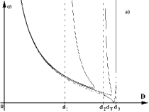
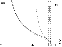
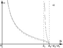
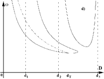
Figure 9: Angular speeds for cases: a) Various positive intensities; b) Positive intensities (two coincide); c) Equal positive intensities; b) One negative intensity.

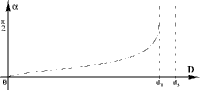
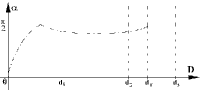
Figure 10: Corners of an inclination for cases: a) Various positive intensities; b) One negative intensity.

In an absolute motion with increase of the moment (mutual distances) angular speed of rotation of Thomson’s configurations monotonously decreases (see Fig. 10), and corner of an inclination normal of a triangle to an axis of rotation grows monotonously also from zero (as for a plane) up to value $\pi/2$ by the moment of merge of Thomson’s and collinear configurations (Fig. 9), by exception of a case equal intensities, when an inclination of an axis change not.

Remark 7. The only possible motions of stationary configurations (i.e. configurations, with distance between vortices do not varies) are the rotations around of some motionless axis. It is a consequence of representability of the equations of vortical dynamics as the first order equations relatively to dynamic variables.

In contrast of Thomson’s configuration, axis of rotation of collinear configurations always lays in a plane of vortices and does not vary by change values of the moment.

With increasing of the moment the diagrams of angular speed are slumped monotonously and disappearance with merging. It is necessary to note large size of angular speeds of vortices, arising at the moment of birth of a new vortex from a problem two vortices. Within the framework of the accepted model this increase of angular speed concerns to different trajectories, but if is present ”weak” dissipation, that it’s possible observe slow evolution both values of energy and moment. Certainly, there are the additional condition existing of such effects in a physical situation more important is the stability of appropriate stationary motions.

Part of collinear configurations, occurring from similar configurations on a plane, are unstable already in linear approach, as it is visible from Fig. 11, because they being analogues configurations on a plane. However collinear configurations, appearing from a problem two vortices, are steady. The nature of this stability is well visible from geometrical interpretation presented on Fig. 8. It is possible, that the phenomena of such grades occurring in an atmosphere of the Earth (that have obviously dissipation). That is crucial for occurrence of various catastrophic processes (type hurricanes), accompanying sharp reorganization of dynamics of vortical formations. Inverse process of collaps (merge) of two vortices, that is impossible for model of an ideal liquid, in case of small dissipation and reduction $D$ can result in formation of atmospheric vortices with large angular speed of rotation.

The Thomson’s solutions are steady up to the moment of passage through static configuration. The analogue of the formula (25) for Thomson’s configurations on sphere is the expression

$$\lambda^{2}=\frac{D-3R^{2}(a_{1}+a_{2}+a_{3})}{9D^{2}}a_{1}a_{2}a_{3}(a_{1}+a_{2}+a_{3}).$$ (35)

That shows, that Tomson’s configuration is unstable with value the moment

$$D>3R^{2}(a_{1}+a_{2}+a_{3}),$$

appropriate to the maximal value, for such configurations.

For a case of one negative intensity $(\Gamma_{1}<0,\quad-\Gamma_{1}>\Gamma_{2}+\Gamma_{3})$ bifurcational diagram is given on Fig. 6d. In this case behaviour bifurcational curves by increase $D$ is similar to behaviour by already considered situations. Existing in case of a plane Thomson’s and collinear configurations merge in a point $A$ (see Fig. 6d), and after this disappear by merging from one of collinear branches, that birth from a problem t of two vortices. Difference from a case only positive by increase $D$ intensities is displayed in existence of collinear solutions, not limited on energy from above. These solutions occur also due to stationary configurations of a problem of two vortices. The change of parameters of an absolute motion of vortices is qualitative by nothing differs from a case positive intensity except for that, that all of collinear configuration are steady, in that time as Thomson’s — is unstable (Fig. 11).

In summary we shall explicitly allocate the basic differences of a spherical case from flat, arising with increase of the complete moment $D:$

1. arising of Thomson’s and collinear configurations on sphere;

2. arising of steady collinear configurations from a problem of two vortices rotating with large (infinite) angular speed in the moment of occurrence;

3. an inclination and evolution of a plane Thomson’s configurations;

4. existence of static configurations on sphere.

Researches of other opportunities of a motion of three vortices on a plane and to sphere resulting to collaps and which is running up to trajectories will be are given in the following part of work.

The authors thank I.S.Mamaev and N.N.Simakov for useful discussions and help in work. The work is carried out under the support of Russian Fond of Fundamental Research (96–01–00747) and Federal programm ”States Support of Integration High Education and Fundamental Science” (project No. 294).

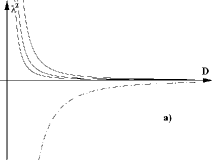
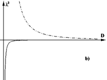
Figure 3: Dependence of a squares of eigenvalues, determining stability in linear approach from integral of complete moment for stationary configurations in a compact case: a) With positive intensities; b) One negative intensity. The dot-dashed line corresponds to the Thomson’s solutions, continuous lines — to collinear configurations.

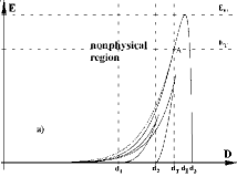
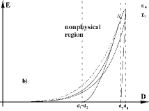
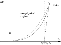
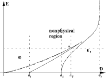
Figure 6: The bifurcational diagram for cases: a) Various positive intensities; b) Positive intensities (two coincide); c) Equal positive intensities; d) One negative intensity. The designations of curves coincide with Fig. 2.

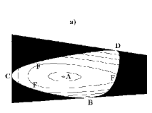
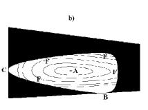
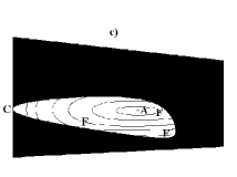
Figure 8: Geometrical picture of birth of collinear solutions from a problem of two vortices. Consecutive figures a), b), c) show change of points of a contact of borders of physically of allowable area with increase of the complete moment. The designations correspond Fig. 1.

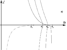
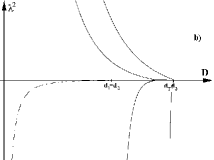
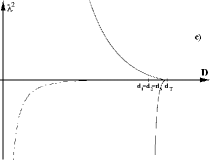
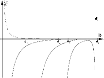
Figure 11: Factor of stability $\lambda^{2}$ for cases: a) Various positive intensities; b) Positive intensities (two coincide); c) Equal positive intensities; d) One negative intensity.

References

- [1] J. J. Thomson. A treatise on the motion of Vortex rings. London: Macmillan, 1883, 124 p.
- [2] W. Gröbli Specialle Probleme über die Bewegung Geredliniger paralleler Wirbelfäden”. Vierteljahrsch. D. Naturforsch. Geselsch. Zürich. V. 22, 1877, P. 37–81, P. 129–165.
- [3] H. Poincaré. Théorie des tourbillous. Paris, 1893, 205 p.
- [4] I. S. Gromeka. On vortex motions of liquid on a Sphere. Collected papers. Moscow, AN USSR, 1952, P. 296 (in Russia).
- [5] A. G. Greenhill. Plane vortex motion. Quat. J. of Pure appl. Math., 1878, V. 15, P. 10–29.
- [6] L. G. Hazin. Regular poligons of point vortices and Resonance instability of stationary states. DAN USSR, V. 230, 1976, No. 4, P.799–802 (in Russian).
- [7] A. Barut, R. Raczka Theory of Group Representations and Applications. PWN. Polish Scientific Publishers, 1977.
- [8] V. A. Bogomolov. Dynamics of vorticity on a sphere. Mech. of liquid and gas, 1977, No. 6, P. 57–65 (in Russian).
- [9] V. A. Bogomolov. Two-dimensional fluid dynamics on a sphere. Izv. Acad. Sci. USSR Atmos. Oceanic Phys., V. 15, 1979, No. 1, P. 29–35 (in Russian).
- [10] H. Aref. Integrable, chaotic and turbulent vortex motion in two-dimensional flows. Ann. Rev. Fluid Mech. V. 15, 1983, P. 345–389.
- [11] V. I. Arnold, V. V. Kozlov, A. I. Neishtadt Mathematical aspects of the classical and selestial mechanics. Moskow: VINITI. Results of a science and engineering. Contemparary problems of mathematics. Fundamental directions, V. 3, 1985, 304 p.
- [12] H. Aref. Motion of three vortices revisited. Phys. Fluids. V. 31, 1988, No. 6, P. 1392–1409.
- [13] N. Rott, H. Aref. Three-vortex motion with zero total circulation. J. Of Appl. Math. And Phys. (ZAMP), V. 40, 1989, P. 473–500.
- [14] V. V. Meleshko, M. Yu. Konstantinov Dynamics of vorticity structure. Kiev, Naukova dumka, 1993, 277 p.
- [15] E. N. Selivanova. Topology of problem of three dot vortices. Works Math. Inst. RAN. V. 205, 1994, P. 141–149.
- [16] A. V. Borisov, K. V Emelyanov Nonintegrability and stochacticity of rigid body dynamics. Izhevsk, Isd-vo Udm. univ., 1995, 57 p.
- [17] A. A. Bagrets, D. A. Bagrets. Nonintegrability of two problems in vortex dynamics. Chaos, V. 7, 1997, Issue 3, P. 368–375.
- [18] A. V. Borisov, A. E. Pavlov. Dynamics and statics of vortices on a plane and a sphere. Reg. & Chaot. Dyn., 1998, V. 3, No. 1, P. 28–38.
- [19] J. Tavantzis, L. Ting. The dynamics of three vortices revised. Phys. Fluids, 1988, V. 31, No. 6, P.1392–1409.
- [20] E. A. Novikov, Yu. B. Sedov. Collaps of vortices. Zh.Eksp.Teor.Fiz., V. 77, 1979, No. 2(8), P. 588–597.
- [21] K. M. Khanin. Quasi-periodic motions of vortex systems. Physica 4D., V. 3, 1982, P. 261-269.