Periodic-Orbit Theory of Universality in Quantum Chaos

Abstract

We argue semiclassically, on the basis of Gutzwiller’s periodic-orbit theory, that full classical chaos is paralleled by quantum energy spectra with universal spectral statistics, in agreement with random-matrix theory. For dynamics from all three Wigner-Dyson symmetry classes, we calculate the small-time spectral form factor $K(\tau)$ as power series in the time $\tau$. Each term $\tau^{n}$ of that series is provided by specific families of pairs of periodic orbits. The contributing pairs are classified in terms of close self-encounters in phase space. The frequency of occurrence of self-encounters is calculated by invoking ergodicity. Combinatorial rules for building pairs involve non-trivial properties of permutations. We show our series to be equivalent to perturbative implementations of the non-linear sigma models for the Wigner-Dyson ensembles of random matrices and for disordered systems; our families of orbit pairs are one-to-one with Feynman diagrams known from the sigma model.

I Introduction

I.1 Background

In the semiclassical limit, fully chaotic quantum systems display universal properties. Universal behavior has been observed for many quantities of interest in such different areas as mesoscopic transport or nuclear physics. One paradigmatic example stands out and will be the object of our investigation: According to the Bohigas-Giannoni-Schmit (BGS) conjecture put forward about two decades ago BGS , highly excited energy levels of generic fully chaotic systems have universal spectral statistics. This conjecture is supported by broad experimental and numerical evidence Stoeckmann ; Haake .

Level statistics can be characterized by the so-called spectral form factor. The level density $\rho(E)=\sum_{i}\delta(E-E_{i})$ of a bounded quantum system ($E_{i}$ denoting the energy levels) is split into a local average $\overline{\rho}(E)$ and an oscillatory part $\rho_{\rm osc}(E)$ describing fluctuations around that average. The form factor is defined as the Fourier transform of the two-point correlator $\langle\rho_{\rm osc}(E+\frac{\epsilon}{2})\rho_{\rm osc}(E-\frac{\epsilon}{2})\rangle$ w.r.t. the energy difference $\epsilon$,

$$K(\tau)=\left\langle\int\!\!\!\frac{d\epsilon}{\overline{\rho}(E)}{\rm e}^{\frac{\rm i}{\hbar}\epsilon\tau T_{H}}\rho_{\rm osc}\!\left(E+\textstyle{\frac{\epsilon}{2}}\right)\rho_{\rm osc}\!\left(E-\textstyle{\frac{\epsilon}{2}}\right)\!\!\right\rangle;$$ (1)

here the time $\tau$, conjugate to the energy difference, is measured in units of the so-called Heisenberg time

$$T_{H}=2\pi\hbar\overline{\rho}(E)=\frac{\Omega(E)}{(2\pi\hbar)^{f-1}}\,,$$ (2)

with $\Omega(E)$ denoting the volume of the energy shell and $f$ the number of freedoms. Since the study of high-lying states justifies the semiclassical limit, we may take $\hbar\to 0,T_{H}\to\infty$, for fixed $\tau$. To make $K(\tau)$ a plottable function, two averages, $\langle\ldots\rangle$ in (1), are necessary, like over windows of the center energy $E$ and a small time interval $\Delta\tau\ll 1$.

Given full chaos, $K(\tau)$ is found to have a universal form, as obtained by averaging over certain ensembles of random matrices Stoeckmann ; Haake ; Mehta . In the absence of geometric symmetries, the prediction of random-matrix theory (RMT) only depends on whether the system in question has no time-reversal (${\cal T}$) invariance (unitary case), or is ${\cal T}$ invariant with either ${\cal T}^{2}=1$ (orthogonal case) or ${\cal T}^{2}=-1$ (symplectic case). RMT yields for $0<\tau<1$

$$K(\tau)=\begin{cases}\tau\hskip 113.81102pt\mbox{unitary;}\\ 2\tau-\tau\ln(1+2\tau)=2\tau-2\tau^{2}+2\tau^{3}-\ldots\\ \hskip 119.50148pt\mbox{orthogonal;}\\ \frac{\tau}{2}-\frac{\tau}{4}\ln(1-\tau)=\frac{\tau}{2}+\frac{\tau^{2}}{4}+\frac{\tau^{3}}{8}+\ldots\\ \hskip 119.50148pt\mbox{symplectic.}\end{cases}$$ (3)

However, a proof of the faithfulness of individual chaotic dynamics to random-matrix theory, and even the assumptions required for a proof, have thus far remained a challenge. In the present paper, we take up the challenge and derive the small-$\tau$ expansion of $K(\tau)$ for individual systems; we employ ergodicity and hyperbolicity of the classical dynamics. Moreover, we require all classical relaxation times (related to Ruelle-Pollicott resonances and Lyapunov exponents) to be finite; we need this property to make sure that even the shortest quantum time scale of relevance, the so-called Ehrenfest time $T_{E}\sim\ln\frac{{\rm const.}}{\hbar}$ is much larger than any classical time scale.

Following Berry ; Argaman ; SR , we start from Gutzwiller’s trace formula Gutzwiller which expresses the level density as a sum over classical periodic orbits $\gamma$,

$$\rho_{\rm osc}(E)\sim\frac{1}{\pi\hbar}{\rm Re}\sum_{\gamma}A_{\gamma}{\rm e}^{{\rm i}S_{\gamma}/\hbar}\,,$$ (4)

wherein $A_{\gamma}$ is the stability amplitude (including the Maslov phase) and $S_{\gamma}$ the action of the $\gamma$th orbit. By (4), the form factor becomes a double sum over orbits,

$$K(\tau)=\frac{1}{T_{H}}\!\!\left\langle\sum_{\gamma,\gamma^{\prime}}\!A_{\gamma}A_{\gamma^{\prime}}^{*}{\rm e}^{\frac{\rm i}{\hbar}(S_{\gamma}-S_{\gamma^{\prime}})}\delta\!\left(\!\!\tau T_{H}-\textstyle{\frac{T_{\gamma}+T_{\gamma^{\prime}}}{2}}\!\!\right)\!\!\!\right\rangle\!;$$ (5)

$T_{\gamma}$ is the period of $\gamma$. For $\hbar\to 0$, only families of orbit pairs with small action difference $|S_{\gamma}-S_{\gamma^{\prime}}|\sim\hbar$ can give a systematic contribution to the form factor. For all others, the phase in (5) oscillates rapidly, and the contribution is killed by the averages indicated. Fluctuations in quantum spectra are thus related to classical correlations among orbit actions Argaman . The first periodic-orbit approach to $K(\tau)$ was taken by Berry Berry , who derived the leading term in (3) using “diagonal” pairs of coinciding ($\gamma^{\prime}=\gamma$) and, for time $\cal T$-invariant dynamics, mutually time-reversed ($\gamma^{\prime}={\cal T}\gamma$) orbits, which obviously are identical in action. Starting with Argaman et al. Argaman , off-diagonal orbit pairs were studied in Cohen ; Primack ; Smilansky . The potential importance of close self-encounters in orbit pairs was first spelled out in work on electronic transport Aleiner and qualitatively discussed for spectral fluctuations in Disorder .

The family of orbit pairs responsible for the next-to-leading order was definitely identified in Sieber’s and Richter’s seminal papers SR for a homogeneously hyperbolic system, the Hadamard-Gutzwiller model (geodesic motion on a tesselated surface of negative curvature with genus 2). Their original formulation was based on small-angle self-crossings of periodic orbits in configuration space. In each pair, the partner $\gamma^{\prime}$ differs from $\gamma$ only by narrowly avoiding one of its many self-crossings. The two orbits almost coincide in one of the two parts separated by the crossing, while they are nearly time-reversed in the other part. In phase space, both orbits contain an “encounter” of two almost time-reversed orbit stretches. They differ only by their connections inside that encounter; see Fig 1.

As shown in Mueller , Sieber’s and Richter’s reasoning can be extended to general fully chaotic two-freedom systems. One partner orbit $\gamma^{\prime}$ arises for each encounter. The action difference within each orbit pair Mueller ; Spehner ; Turek can be derived using the geometry of the invariant manifolds Braun . It thus turned out helpful to reformulate the treatment in terms of phase-space coordinates Spehner ; Turek , which may also be applied to systems with more than two freedoms Higherdim .

In Tau3 , we showed that the $\tau^{3}$-contribution to the form factor originates from pairs of orbits which differ either in two encounters of the above kind, or in one encounter that involves three orbit stretches.

In the present paper we demonstrate how the whole series expansion of $K(\tau)$ is obtained from periodic orbits. Beyond furnishing details left out in our previous letter Letter we here cover systems with more than two freedoms and from all three Wigner-Dyson symmetry classes. For the symplectic case we employ ideas presented in Heusler ; BolteHarrison . For related work on quantum graphs, see Berkolaiko for the first three orders of $K(\tau)$ and GnutzAlt for a complete treatment.

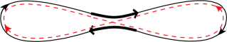
Figure 1: Sketch of a Sieber/Richter pair in configuration space: The partner orbits, depicted by solid and dashed lines, differ noticeably only inside an encounter of two orbit stretches (marked by antiparallel arrows, indicating the direction of motion). The sketch greatly exaggerates the difference between the two partner orbits in the loops outside the encounter and depicts the loops disproportionally short; similar remarks apply to all subsequent sketches of orbit pairs.

I.2 Overview

We set out to identify the families of orbit pairs responsible for all orders of the $\tau$-expansion. The key point is that long orbits have a huge number of close self-encounters which may involve arbitrarily many orbit stretches. We speak of an $l$-encounter whenever $l$ stretches of an orbit get “close” in phase space. “Closeness” will be quantified below such that we may speak of the beginning, the end, and the duration of an encounter. Fig. 2a highlights two such encounters inside a periodic orbit, one 2-encounter and one 4-encounter. Here, as always, we sketch orbit pairs in configuration space, with arrows $\mathrel{\,\lower 0.6458pt\hbox{\begin{picture}(4.0,3.0)\put(0.0,0.8){\vector(1,0){4.0}}\put(0.0,2.0){\vector(1,0){4.0}}\end{picture}}\,}$ indicating the direction of motion inside the encounter stretches. The relevant encounters will turn out to have durations of the order of the Ehrenfest time $T_{E}\sim\ln\frac{\rm{const.}}{\hbar}$; even though logarithmically divergent in the semiclassical limit (and thus larger than all classical time scales), these encounter durations are vanishingly small compared to the orbit periods, which are of the order of the Heisenberg time, $T_{\gamma}\sim T_{H}\sim\hbar^{-f+1}$. In between different self-encounters an orbit goes through “loops”, represented by thin full lines.

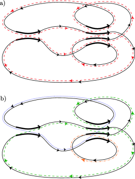
Figure 2: a) Solid line: Periodic orbit $\gamma$ with one 4-encounter and one 2-encounter highlighted by bold arrows. Dotted line: Partner $\gamma^{\prime}$ differing from $\gamma$ by connections in the encounters. b) Other reconnections yield a “pseudo-orbit” decomposing into three periodic orbits (dashed, dotted, and dash-dotted).

Self-encounters are of interest since they lead us from a periodic orbit $\gamma$ to partners $\gamma^{\prime}$ which differ from $\gamma$ noticeably only inside a set of encounters (see the dashed orbit in 2a). In contrast, the orbit loops in between encounters are almost identical. The almost coinciding loops of $\gamma$ and $\gamma^{\prime}$ are differently connected inside the encounters.

Not all reshufflings of connections inside an encounter yield a partner orbit. For example, reconnections as in Fig. 2b give rise to a “pseudo-orbit” decomposing into three separate periodic orbits. Pseudo-orbits are not admitted in the Gutzwiller trace formula.

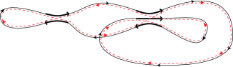
Figure 3: Periodic orbit $\gamma$ with one 2- and one 3-encounter highlighted, and a partner $\gamma^{\prime}$ obtained by reconnection; the encounters depicted only exist in ${\cal T}$-invariant systems.

For ${\cal T}$-invariant dynamics, we also must account for encounters whose stretches only get close up to time reversal as in $\mathrel{\,\lower 0.6458pt\hbox{\begin{picture}(4.0,3.0)\put(4.0,0.3){\vector(-1,0){4.0}}\put(0.0,1.5){\vector(1,0){4.0}} \put(0.0,2.7){\vector(1,0){4.0}} \end{picture}}\,}$ and $\mathrel{\,\lower 0.6458pt\hbox{\begin{picture}(4.0,3.0)\put(4.0,0.8){\vector(-1,0){4.0}}\put(0.0,2.0){\vector(1,0){4.0}} \end{picture}}\,}$; see Fig. 3. Correspondingly, loops inside mutual partner orbits may be related by time reversal.

We thus obtain a natural extension of Berry’s diagonal approximation. Instead of considering only pairs of orbits which exactly coincide (or are mutually time-reversed), we employ all pairs whose members are composed of similar (up to time reversal) loops.

We proceed to classify these orbit pairs. Partner orbits may differ in a number $v_{l}$ of $l$-encounters; we shall assemble these numbers to a “vector” $\vec{v}=(v_{2},v_{3},\ldots)$. The total number of encounters is given by $V=\sum_{l\geq 2}v_{l}$. The number of orbit stretches involved in encounters, coinciding with the number of intervening loops, reads $L=\sum_{l\geq 2}lv_{l}$.

The orbit pairs $(\gamma,\gamma^{\prime})$ related to a fixed vector $\vec{v}$ may have various structures. Each structure corresponds to a different ordering (and, given ${\cal T}$-invariance, different sense of traversal) of the loops of $\gamma$ inside the partner orbit $\gamma^{\prime}$. When drawing orbit pairs as in Figs. 2 and 3, these structures differ by the order in which encounters are visited in the original orbit $\gamma$, and by the relative directions of the stretches within each encounter (i.e. $\mathrel{\,\lower 0.6458pt\hbox{\begin{picture}(4.0,3.0)\put(0.0,0.8){\vector(1,0){4.0}}\put(0.0,2.0){\vector(1,0){4.0}}\end{picture}}\,}$ vs. $\mathrel{\,\lower 0.6458pt\hbox{\begin{picture}(4.0,3.0)\put(4.0,0.8){\vector(-1,0){4.0}}\put(0.0,2.0){\vector(1,0){4.0}} \end{picture}}\,}$, or $\mathrel{\,\lower 0.6458pt\hbox{\begin{picture}(4.0,3.0)\put(0.0,0.3){\vector(1,0){4.0}}\put(0.0,1.5){\vector(1,0){4.0}} \put(0.0,2.7){\vector(1,0){4.0}} \end{picture}}\,}$ vs. $\mathrel{\,\lower 0.6458pt\hbox{\begin{picture}(4.0,3.0)\put(4.0,0.3){\vector(-1,0){4.0}}\put(0.0,1.5){\vector(1,0){4.0}} \put(0.0,2.7){\vector(1,0){4.0}} \end{picture}}\,}$ in time-reversal invariant systems). Moreover, different reconnections inside the same encounter may give rise to different partners, and hence different structures. We will see that structures have a one-to-one correspondence to permutations, which will be used in Section III to determine the number $N(\vec{v})$ of structures related to the same $\vec{v}$.

Orbit pairs sharing the same $\vec{v}$ and the same structure may still differ in the phase-space separations between the encounter stretches. We shall parametrize those separations by suitable variables $s$, $u$ and determine their density $w_{T}(s,u)$ inside orbits of period $T$. The double sum (5) over orbits defining the spectral form factor will be written as a sum of contributions from families of orbit pairs, with the family weight $\propto N(\vec{v})w_{T}(s,u)$.

This paper is organized as follows. To free the presentation of unnecessary details we mostly disregard complications due to $f>2$ and “non-homogeneous” hyperbolicity (i.e. Lyapunov exponents different for different periodic orbits). In Section II, we will study the phase-space geometry of encounters and derive the density $w_{T}(s,u)$. The purely combinatorial task of determining the number of structures $N(\vec{v})$ is attacked in Section III with the help of the theory of permutations. We thus obtain series expansions of $K(\tau)$ for individual chaotic systems with and without ${\cal T}$-invariance; those series fully coincide with the RMT predictions for the Gaussian orthogonal ensemble (GOE) and the Gaussian unitary ensemble (GUE), respectively. Section IV generalizes these results to systems where spin dynamics accompanies translational motion; in particular, we find agreement with the Gaussian Symplectic Ensemble (GSE) given ${\cal T}$-invariance with ${\cal T}^{2}=-1$. In Section V, we show that our semiclassical procedure bears a close analogy to quantum field theory. In fact, our families of orbit pairs are equivalent to Feynman diagrams met within the theory of disordered systems and the perturbative implementation of the so-called nonlinear sigma model. Finally, we present conclusions in Section VI. Further details, including a generalization to $f>2$ and non-homogeneous hyperbolicity, and remarks on the action correlation function of Argaman , are given in Appendices.

II Phase-space geometry of encounters

II.1 Fully chaotic dynamics

At issue are fully chaotic, i.e., hyperbolic and ergodic Hamiltonian flows without geometric symmetries with $f=2$ “classical” freedoms. In the orthogonal case, the Hamiltonian is assumed to be ${\cal T}$ invariant, ${\cal T}H{\cal T}^{-1}=H$, with an anti-unitary time-reversal operator ${\cal T}$ squaring to unity. For convenience, we assume ${\cal T}$ to be the conventional time-reversal operator ${\cal T}({\bf q},{\bf p})=({\bf q},-{\bf p})$; that assumption does not restrict generality, since all Hamiltonians with non-conventional time-reversal invariance can be brought to conventionally time-reversal invariant form by a suitable canonical transformation Braun .

For each phase-space point ${\bf x}=({\bf q},{\bf p})$ it is possible to define a Poincaré surface of section ${\cal P}$ orthogonal to the trajectory passing through ${\bf x}$. Assuming a Cartesian configuration space (and thus a Cartesian momentum space), ${\cal P}$ consists of all points ${\bf x}+\delta{\bf x}=({\bf q}+\delta{\bf q},{\bf p}+\delta{\bf p})$ in the same energy shell as ${\bf x}$ whose configuration-space displacement $\delta{\bf q}$ is orthogonal to ${\bf p}$. For $f=2$, ${\cal P}$ is a $2$-dimensional surface within the $3$-dimensional energy shell. Given hyperbolicity, ${\cal P}$ is spanned by one stable direction ${\bf e}^{s}({\bf x})$ and one unstable direction ${\bf e}^{u}({\bf x})$ Gaspard . We may thus decompose $\delta{\bf x}$ as

$$\delta{\bf x}=\hat{s}{\bf e}^{s}({\bf x})+\hat{u}{\bf e}^{u}({\bf x})\,.$$ (6)

As long as two trajectories passing respectively through ${\bf x}$ and ${\bf x}+\delta{\bf x}$ remain sufficiently close, we may follow their separation by linearizing the equations of motion around one trajectory,

$$\hat{s}(t) = \Lambda({\bf x},t)^{-1}\hat{s}(0)$$

$$\hat{u}(t) = \Lambda({\bf x},t)\hat{u}(0)\,.$$ (7)

Here, $\hat{s}(t)$ and $\hat{u}(t)$ denote stable and unstable components in a co-moving Poincaré section at ${\bf x}(t)$, the image of ${\bf x}={\bf x}(0)$ under time evolution over time $t$. In the long-time limit, the fate of the stretching factor $\Lambda({\bf x},t)$ and thus of the stable and unstable components is governed by the (local) Lyapunov exponent $\lambda({\bf x})>0$

$$\Lambda({\bf x},t)\sim{\rm e}^{\lambda({\bf x})t}\,.$$ (8)

The ${\bf x}$-dependence of $\lambda$ and $\Lambda$ will be relevant only in Appendix B.1, when we treat non-homogeneous hyperbolicity; until then, we may think of these quantities as constants. As in Spehner ; Turek ; Higherdim , the directions ${\bf e}^{s}({\bf x})$ and ${\bf e}^{u}({\bf x})$ are mutually normalized by fixing their symplectic product as

$${\bf e}^{u}({\bf x})\land{\bf e}^{s}({\bf x})={\bf e}^{u}({\bf x})^{T}\left(\begin{array}[]{cc}0&-1\\ 1&0\end{array}\right){\bf e}^{s}({\bf x})=1\,.$$ (9)

In ergodic systems, almost all trajectories fill the corresponding energy shell uniformly. The time average of any observable along such a trajectory coincides with an energy-shell average.

Periodic orbits are exceptional in the sense that they cannot visit the whole energy shell. However, long periodic orbits still behave ergodically: According to the equidistribution theorem Equidistribution (see also Appendix B.1), a time average over an orbit $\gamma$ augmented by an average over all $\gamma$ from a small time window, with the squared stability coefficient as a weight, equals the energy-shell average with the Liouville measure. A special case is the sum rule of Hannay and Ozorio de Almeida HOdA

$$\left\langle\sum_{\gamma}|A_{\gamma}|^{2}\delta(T-T_{\gamma})\right\rangle_{\Delta T}=T\,.$$ (10)

Ergodicity makes, in the limit of long times, for a uniform return probability: A trajectory starting at ${\bf x}$ again pierces through ${\cal P}$ in a time interval $(t,t+dt)$ with stable and unstable components of ${\bf x}(t)-{\bf x}(0)$ (or ${\cal T}{\bf x}(t)-{\bf x}(0)$) lying in intervals $(\hat{s},\hat{s}+d\hat{s})$, $(\hat{u},\hat{u}+d\hat{u})$ with uniform probability $\frac{1}{\Omega}d\hat{s}d\hat{u}dt$.

II.2 Encounters

To parametrize an $l$-encounter, we introduce a Poincaré surface of section ${\cal P}$ transversal to the orbit at an arbitrary phase-space point ${\bf x}_{1}$ (passed at time $t_{1}$) inside one of the encounter stretches. The exact location of ${\cal P}$ inside the encounter is not important. The remaining stretches pierce through ${\cal P}$ at times $t_{j}$ ($j=2,\ldots,l$) in points ${\bf x}_{j}$. If the $j$-th encounter stretch is close to the first one in phase space, we must have ${\bf x}_{j}\approx{\bf x}_{1}$; if it is almost time-reversed with respect to the first one, we have ${\cal T}{\bf x}_{j}\approx{\bf x}_{1}$. In the sequel, we shall shorthand as ${\bf y}_{j}\approx{\bf x}_{1}$ with ${\bf y}_{j}$ either ${\bf x}_{j}$ or ${\cal T}{\bf x}_{j}$.

The small difference ${\bf y}_{j}-{\bf x}_{1}$ can be decomposed in terms of the stable and unstable directions at ${\bf x}_{1}$,

$${\bf y}_{j}-{\bf x}_{1}=\hat{s}_{j}{\bf e}^{s}({\bf x}_{1})+\hat{u}_{j}{\bf e}^{u}({\bf x}_{1})\,;$$ (11)

the stable and unstable components $\hat{s}_{j}$, $\hat{u}_{j}$ depend on the location ${\bf x}_{1}$ of the Poincaré section ${\cal P}$ chosen within the encounter. If we shift ${\cal P}$ through the encounter, the stable components will asymptotically decrease and the unstable components will asymptotically increase with growing $t_{1}$, according to (II.1,8).

We can now give a more precise definition of an $l$-encounter. To guarantee that all $l$ stretches are mutually close, we demand the stable and unstable differences $|\hat{s}_{j}|$, $|\hat{u}_{j}|$ of all stretches from the first one to be smaller than a constant $c$. The bound $c$ must be chosen small enough for the motion around the $l$ orbit stretches to allow for the mutually linearized treatment (II.1); however, the exact value of $c$ is irrelevant.

The stable and unstable coordinates determine the duration $t_{\rm enc}$ of an encounter. We have to sum the durations of the “head” of the encounter (i.e. the time $t_{u}$ until the end of the encounter, when the first of the unstable components $|\hat{u}_{j}|$ reaches $c$) and its “tail” (i.e. the time $t_{s}$ passed since the beginning of the encounter, when the last of the stable components $|\hat{s}_{j}|$ has fallen below $c$). Using the exponential divergence of the unstable phase-space separations (8), we see that the coordinates $|\hat{u}_{j}|$ approximately need the time $\frac{1}{\lambda}\ln\frac{c}{|\hat{u}_{j}|}$ to reach $c$; similarly, the stable coordinates need $\frac{1}{\lambda}\ln\frac{c}{|\hat{s}_{j}|}$. We thus obtain

$$t_{u} = \min_{j}\left\{\frac{1}{\lambda}\ln\frac{c}{|\hat{u}_{j}|}\right\}\,,\quad t_{s}=\min_{j}\left\{\frac{1}{\lambda}\ln\frac{c}{|\hat{s}_{j}|}\right\}\,,$$

$$t_{\rm enc} = t_{s}+t_{u}=\frac{1}{\lambda}\ln\frac{c^{2}}{\max_{i}\{|\hat{s}_{i}|\}\max_{j}\{|\hat{u}_{j}|\}}\,;$$ (12)

in view of (II.1), the duration $t_{\rm enc}$ remains invariant if the Poincaré section ${\cal P}$ is shifted through the encounter.

An $l$-encounter involves $l$ different orbit stretches whose initial and final phase-space points will be referred to as “entrance” and ”exit ports”. If all encounter stretches are (almost) parallel, as in $\mathrel{\,\lower 0.6458pt\hbox{\begin{picture}(4.0,3.0)\put(0.0,0.3){\vector(1,0){4.0}}\put(0.0,1.5){\vector(1,0){4.0}} \put(0.0,2.7){\vector(1,0){4.0}} \end{picture}}\,}$, all entrance ports are located on the same side of the encounter, and the exit ports are located on the opposite side. If the encounter involves mutually time-reversed orbit stretches as $\mathrel{\,\lower 0.6458pt\hbox{\begin{picture}(4.0,3.0)\put(4.0,0.3){\vector(-1,0){4.0}}\put(0.0,1.5){\vector(1,0){4.0}} \put(0.0,2.7){\vector(1,0){4.0}} \end{picture}}\,}$, this is no longer the case. Thus, it is useful to introduce the following convention: All ports on the side where the first stretch begins are called “left ports”, while those on the opposite side are ”right ports”. For parallel encounters, “entrance” and “left” are synonymous, as well as “exit” and “right”.

II.3 Partner orbits

The partner orbits $(\gamma,\gamma^{\prime})$ differ from one another only inside the encounters, by their connections between left and right ports. We shall number these ports in order of traversal by $\gamma$, such that the $i$-th encounter stretch of $\gamma$ connects left port $i$ to right port $i$. Inside $\gamma^{\prime}$, the left port $i$ is connected to a different right port $j$; see Fig. 4a.

We must reshuffle connections between all stretches of a given encounter. In contrast, Fig. 4b shows reconnections only between stretches 1 and 2, stretches 3 and 4, and between stretches 5 and 6 of a 6-encounter which therefore decomposes into three 2-encounters.

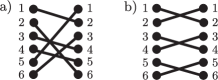
Figure 4: Connections between left and right ports in partner orbit $\gamma^{\prime}$. In b), the encounter splits into three pieces respectively containing the two upper, middle, and lower stretches.

II.3.1 Piercing points

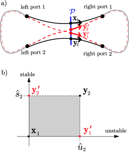
Figure 5: Piercings ${\bf x}_{1}$, ${\bf y}_{2}$ of $\gamma$ (full line) and piercings ${\bf y}_{1}^{\prime}$, ${\bf y}_{2}^{\prime}$ of $\gamma^{\prime}$ (dashed line) for a Sieber/Richter pair, depicted a) in configuration space, with arrows indicating the momentum of the above phase-space points, and b) in the Poincaré section ${\cal P}$ parametrized by stable and unstable coordinates. The symplectic area of the rectangle is the action difference $\Delta S$.

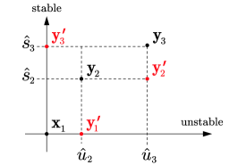
Figure 6: Piercing points of $\gamma$,$\gamma^{\prime}$ differing in a 3-encounter; inside $\gamma^{\prime}$, left ports 1,2,3 are connected to right ports 2,3,1, respectively.

The partner $\gamma^{\prime}$ also pierces through our Poincaré section ${\cal P}$. The corresponding piercing points are determined by those of $\gamma$. In particular, the unstable coordinates of a piercing point depend on the following right port. If two stretches of $\gamma$ and $\gamma^{\prime}$ lead to the same right port, they have to approach each other for a long time - at least until the end of the encounter (which has a duration $\sim T_{E}$) and half-way through the subsequent loop. Hence, their difference must be close to the stable manifold, and the unstable coordinates almost coincide. Similarly, the stable coordinates are determined by the previous left port, since stretches with the same left port approach for large negative times. If a stretch of $\gamma^{\prime}$ connects left port $i$ to right port $j$, it thus pierces through our Poincaré section with stable and unstable coordinates

$$\hat{s}_{i}^{\prime}\approx\hat{s}_{i},\ \ \ \ \hat{u}_{i}^{\prime}\approx\hat{u}_{j}.$$ (13)

For instance, if $\gamma$ and $\gamma^{\prime}$ differ in a 2-encounter, $\gamma^{\prime}$ connects left port 1 to right port 2, and left port 2 to right port 1; see Fig. 5a. Thus, the encounter stretches of $\gamma^{\prime}$ pierce through ${\cal P}$ in ${\bf y}^{\prime}_{1}$ with $\hat{s}^{\prime}_{1}\approx\hat{s}_{1}=0$, $\hat{u}^{\prime}_{1}\approx\hat{u}_{2}$, and in ${\bf y}^{\prime}_{2}$ with $\hat{s}^{\prime}_{2}\approx\hat{s}_{2}$, $u^{\prime}_{2}\approx\hat{u}_{1}=0$, which together with the piercings of $\gamma$ span a parallelogram in phase space Braun (a rectangle in Fig. 5b, by artist’s license). In Fig. 6, we visualize the locations of ${\bf y}^{\prime}_{j}$ inside ${\cal P}$ for a 3-encounter.

II.3.2 Action difference

We can now determine the difference between the actions of the two partner orbits, first for $\gamma$, $\gamma^{\prime}$ only differing in one 2-encounter. Generalizing the results for configuration-space crossings in SR ; Mueller , we will show that the action difference is just the symplectic area of the rectangle in Fig. 5b Spehner ; Turek . Consider two segments of the encounter stretches in Fig. 5a, leading from the first left port to the piercing point ${\bf x}_{1}$ of $\gamma$, and to the piercing point ${\bf y}_{1}^{\prime}$ of $\gamma^{\prime}$, respectively. Since the action variation brought about by a shift $d{\bf q}$ of the final coordinate is ${\bf p}\cdot d{\bf q}$, the action difference between the two segments will be given by $\Delta S^{(1)}=\int_{{\bf y}_{1}^{\prime}}^{{\bf x}_{1}}{\bf p}\cdot d{\bf q}$. The integration line may be chosen to lie in the Poincaré section; then it coincides with the unstable axis. Repeating the same reasoning for the remaining segments, we obtain the overall action difference $\Delta S\equiv S_{\gamma}-S_{\gamma^{\prime}}$ as the line integral $\Delta S=\oint{\bf p}\cdot d{\bf q}$ along the contour of the parallelogram ${\bf y}^{\prime}_{1}\to{\bf x}_{1}\to{\bf y}^{\prime}_{2}\to{\bf y}_{2}\to{\bf y}^{\prime}_{1}$, spanned by ${\bf y}_{1}^{\prime}-{\bf x}_{1}=\hat{u}_{2}{\bf e}^{u}({\bf x}_{1})$ and ${\bf y}_{2}^{\prime}-{\bf x}_{1}=\hat{s}_{2}{\bf e}^{s}({\bf x}_{1})$. This integral indeed gives the symplectic area

$$\Delta S=\hat{u}_{2}{\bf e}^{u}({\bf x}_{1})\land\hat{s}_{2}{\bf e}^{s}({\bf x}_{1})=\hat{s}_{2}\hat{u}_{2}\,.$$ (14)

To generalize to arbitrary $l$-encounters, we imagine a partner orbit $\gamma^{\prime}$ constructed out of $\gamma$ by $l-1$ successive steps, as illustrated for a special example in Fig. 7. Each step interchanges the right ports of two encounter stretches and contributes to the action difference an amount given by (14). At the same time, the two piercings points change their position as discussed in 6. This step-by-step process suggests a useful transformation of coordinates. Let $s_{j}$, $u_{j}$ denote the stable and unstable differences between the two stretches affected by the $j$-th step. Note that in contrast to $\hat{s}_{j}$, $\hat{u}_{j}$ the index $j$ no longer represents encounter stretches $2,\ldots,l$ but steps $1,\ldots,(l-1)$. Now, the change of action in each step is simply given by $s_{j}u_{j}$. Summing over all steps, we obtain a total action difference

$$\Delta S=\sum_{j=1}^{l-1}s_{j}u_{j}\,.$$ (15)

The transformation leading from $\hat{s}_{j}$, $\hat{u}_{j}$ to $s_{j}$, $u_{j}$ is linear and volume-preserving. Due to the elegant form of (15), it will be convenient to use $s_{j}$, $u_{j}$ rather than $\hat{s}_{j}$, $\hat{u}_{j}$ in defining the encounter regions, demanding all $|s_{j}|$, $|u_{j}|$ to be smaller than our bound $c$. Employing (II.1), one easily shows that $\Delta S$ remains invariant if the Poincaré section ${\cal P}$ is shifted through the encounter. Moreover, if the orbits $\gamma$ and $\gamma^{\prime}$ differ in several encounters, the total action difference is additive in their contributions, and each is given by (15).

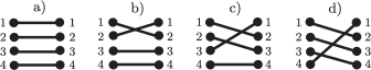
Figure 7: Steps from connections in $\gamma$ (depicted in a) to those in $\gamma^{\prime}$ (shown in d), in each step interchanging right ports of two encounter stretches.

At this point, we can finally appreciate that the encounters relevant for spectral universality have a duration of the order of the Ehrenfest time. The form factor is determined by orbit pairs with an action difference $\Delta S$ of order $\hbar$. According to our expression (14) for $\Delta S$, the relevant stable and unstable coordinates are of the order $\sqrt{\hbar}$. The encounter duration, logarithmic in $s$ and $u$, must consequently be of the order of the Ehrenfest time.

II.4 Structures

We want to define more precisely the notion of “structures” of orbit pairs $\gamma$, $\gamma^{\prime}$.

(i) First of all, these structures are characterized by the order in which encounters are traversed in $\gamma$. We enumerate the encounter stretches of $\gamma$ in their order of traversal, starting from some arbitrarily chosen stretch, and assemble the labels $1\ldots L(\vec{v})$ in $V=V(\vec{v})$ groups according to the encounters they belong to. Such a division uniquely defines the order in which the encounters are visited. For example, in an orbit pair differing in two 2-encounters the four stretches can be distributed among the encounters as (1,2)(3,4) or (1,3)(2,4) or (1,4)(2,3); each of these three possibilities determines a different structure.

Some structures refer to the same orbit pair. Indeed, a different choice of the initial stretch in the same $\gamma$ would lead to a cyclic shift in the enumeration of stretches, and that shift may change the structure associated with $\gamma$. In the example of two 2-encounters, cyclic shifts may either leave the structure (1,2)(3,4) invariant or turn it into (1,4)(2,3), such that the structures (1,2)(3,4) and (1,4)(2,3) are physically equivalent.

Moreover, structures are characterized (ii) by the relative directions of the encounter stretches (i.e. $\mathrel{\,\lower 0.6458pt\hbox{\begin{picture}(4.0,3.0)\put(0.0,0.8){\vector(1,0){4.0}}\put(0.0,2.0){\vector(1,0){4.0}}\end{picture}}\,}$ or $\mathrel{\,\lower 0.6458pt\hbox{\begin{picture}(4.0,3.0)\put(4.0,0.8){\vector(-1,0){4.0}}\put(0.0,2.0){\vector(1,0){4.0}} \end{picture}}\,}$ for 2-encounters, and $\mathrel{\,\lower 0.6458pt\hbox{\begin{picture}(4.0,3.0)\put(0.0,0.3){\vector(1,0){4.0}}\put(0.0,1.5){\vector(1,0){4.0}} \put(0.0,2.7){\vector(1,0){4.0}} \end{picture}}\,}$ or $\mathrel{\,\lower 0.6458pt\hbox{\begin{picture}(4.0,3.0)\put(4.0,0.3){\vector(-1,0){4.0}}\put(0.0,1.5){\vector(1,0){4.0}} \put(0.0,2.7){\vector(1,0){4.0}} \end{picture}}\,}$ for 3-encounters in ${\cal T}$ invariant systems), and (iii) by the reconnections leading from $\gamma$ to $\gamma^{\prime}$; the latter distinction is important if there exist several such reconnections inside the same encounter set, each leading to a different connected partner.

II.5 Statistics of encounter sets

The statistics of close self-encounters inside periodic orbits can be established using the ergodicity of the classical motion. As a second ingredient, it is important to only consider sets of encounters whose stretches are separated by non-vanishing loops, i.e. do not overlap. For example, if two stretches of different encounters overlap, the two encounters effectively merge, leaving one larger encounter with more internal stretches, see Fig. 8. The partners are thus seen as differing in one larger encounter, rather than in two smaller ones. For the more involved case of stretches belonging to the same encounter, see Appendix D.

In the following, we will consider encounter sets within orbit pairs $(\gamma,\gamma^{\prime})$ with fixed $\vec{v}$ and fixed structure. Each of the $V$ encounters of $\gamma$ is parametrized with the help of a Poincaré section ${\cal P}_{\alpha}$ ($\alpha=1,\ldots,V$) crossing the orbit at an arbitrary phase-space point inside the encounter, traversed at time $t_{\alpha 1}$. The orbit again pierces through these sections at times $t_{\alpha j}$ with $j=2,\ldots,l_{\alpha}$ numbering the remaining stretches of the $\alpha$-th encounter. The first piercing may occur anywhere inside the orbit at a time $0<t_{11}<T$, $T$ denoting the period. The remaining $t_{\alpha j}$ follow in an order fixed by the structure at times $t_{11}<t_{\alpha j}<T+t_{11}$. Each of the $v_{l}$ $l$-encounters is characterized by $l-1$ stable and unstable coordinates $s_{\alpha j}$, $u_{\alpha j}$ ($j=1,\ldots,l-1$), which in total make for $2\sum_{l\geq 2}(l-1)v_{l}=2(L-V)$ components. If ${\cal P}_{\alpha}$ is shifted through the encounter, the stable and unstable coordinates change while the contributions to the action difference $\Delta S_{\alpha j}=s_{\alpha j}u_{\alpha j}$ remain invariant.

We proceed to derive a density $w_{T}(s,u)$ of phase-space separations $s$, $u$. To understand the normalization of $w_{T}(s,u)$, assume that it is multiplied with $\prod_{\alpha j}\delta(\Delta S_{\alpha j}-s_{\alpha j}u_{\alpha j})$ and integrated over all $s$, $u$. The result will be the average density of partners $\gamma^{\prime}$ per one orbit $\gamma$ such that the pair $(\gamma,\gamma^{\prime})$ has the given structure and action difference components $\Delta S_{\alpha j}$. Averaging will be carried out over the ensemble of all periodic orbits $\gamma$ with period $T$ in a given time window, assuming that the contribution of each orbit is weighted with the square of its stability amplitude. According to the equidistribution theorem this ensemble is ergodic yielding the same averages as integrating over the energy shell with the Liouville measure.

We need to count the piercings through Poincaré sections parametrized by stable and unstable coordinates. Due to ergodicity, the expected number of such piercings through a given section in the time interval $(t,t+dt)$ with stable and unstable components in $(\hat{s},\hat{s}+d\hat{s})\times(\hat{u},\hat{u}+d\hat{u})$ is equal to $d\hat{s}\;d\hat{u}\;dt/\Omega$, i.e. corresponds to the uniform Liouville density $1/\Omega$.

In fact, we need the number of sets of $L-V$ piercings through our sections ${\cal P}_{\alpha}$ occurring in time intervals $(t_{\alpha j},t_{\alpha j}+dt_{\alpha j})$, $j=2,\ldots,l_{\alpha}$, with stable and unstable coordinates inside $(s_{\alpha j},s_{\alpha j}+ds_{\alpha j})$, $(u_{\alpha j},u_{\alpha j}+du_{\alpha j})$, $j=1,\ldots,l_{\alpha}-1$; that number will be denoted by $\rho_{T}(s,u)\,d^{L-V}s\,d^{L-V}u\,d^{L-V}t$. The uniform Liouville density carries over to the coordinates $s_{\alpha j},u_{\alpha j}$ since the transformation from $\hat{s},\hat{u}$ to $s,u$ is volume-preserving; so we may expect $\rho_{T}(s,u)$ equal to $1/\Omega^{L-V}$.

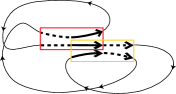
Figure 8: Two 2-encounters (marked by boxes) overlap in one stretch and thus merge to a 3-encounter (solid bold arrows)

However, recall that we are only interested in encounters separated by non-vanishing loops. To implement that restriction, we employ a suitable characteristic function $\Theta_{T}(s,u,t)$ which vanishes if the piercings described by $s$, $u$ and $t$ correspond to overlapping stretches, and otherwise equals $1$. We thus obtain

$$\rho_{T}(s,u,t)=\Theta_{T}(s,u,t)\frac{1}{\Omega^{L-V}}\,.$$ (16)

(Actually the duration of the connecting loops must be not just positive but also larger than all classical relaxation times describing correlation decay, to guarantee the statistical independence of the piercings. However, that classical minimal loop length $t_{\rm cl}$ is not worth further mention since it is vanishingly small compared to the Ehrenfest time, the smallest time scale of semiclassical relevance.)

Proceeding towards $w_{T}(s,u)$ we integrate over the $L-V$ piercing times $t_{\alpha j}$, $j\geq 2$, still for fixed Poincaré sections ${\cal P}_{\alpha}$. The integral yields a density of the stable and unstable components $s$, $u$ of $L-V$ piercings, reckoned from the $V$ reference piercings. To finally get to $w_{T}$, we must keep track of all encounters along the orbits in question. To that end we have to consider all possible positions of Poincaré sections and thus integrate over the times $t_{\alpha 1}$ (of the reference piercings) as well. Doing so, we weigh each encounter with its duration $t_{\rm enc}^{\alpha}$, since we may move each Poincaré section to any position inside the duration of the encounter. In order to count each encounter set exactly once, we divide out the factors $t_{\rm enc}^{\alpha}$, and thus arrive at the desired density

$$w_{T}(s,u)=\frac{\int d^{L}t\,\Theta_{T}(s,u,t)}{\prod_{\alpha}t_{\rm enc}^{\alpha}\,\Omega^{L-V}}\,.$$ (17)

It remains to evaluate the $L$-fold time integral in (17). The integration over $t_{11}$ runs from 0 to $T$; it will be done as the last integral and then give a factor $T$. The $L-1$ other $t_{\alpha j}$ must lie inside the interval $(t_{11},t_{11}+T)$ and respect the ordering dictated by the encounter structure. Moreover, subsequent encounter stretches must not overlap. Thus, the time between the piercings of two subsequent stretches must be so large as to contain both the head of the first stretch and, after a non-vanishing loop, the tail of the second stretch. (Given ${\cal T}$-invariance, we rather need to include the tail of the first stretch, if it is time-reversed w. r. t. the earliest stretch of its encounter; likewise the second stretch may also participate with its head.) These minimal distances sum up to the total duration of all encounter stretches $\sum_{\alpha}l_{\alpha}t_{\rm enc}^{\alpha}$, since each stretch appears in this sum once with head and tail.

The minimal distances effectively reduce the integration range, as we may proceed to a new set of times $\tilde{t}_{\alpha j}$ obtained by subtracting from $t_{\alpha j}$ both $t_{11}$ and the sum of minimal distances between $t_{11}$ and $t_{\alpha j}$. The $\tilde{t}_{\alpha j}$ just have to obey the ordering in question, and lie in an interval $(0,T-\sum_{\alpha}l_{\alpha}t_{\rm enc}^{\alpha})$, where the subtrahend is the total sum of minimal distances. We are thus left with a trivial integral over a constant. Perhaps surprisingly, the resulting density

$$w_{T}(s,u)=\frac{T(T-\sum_{\alpha}l_{\alpha}t_{\rm enc}^{\alpha})^{L-1}}{(L-1)!\prod_{\alpha}t_{\rm enc}^{\alpha}\Omega^{L-V}}$$ (18)

depends only on $\vec{v}$ but not on the structure considered, and that fact strongly simplifies our treatment.

The number $P_{\vec{v}}(\Delta S)d\Delta S$ of orbit pairs with given $\vec{v}$ and action difference within $(\Delta S,\Delta S+d\Delta S)$ now reads

$$\!\!\!\!\!\!P_{\vec{v}}(\Delta S)d\Delta S=d\Delta S\frac{N(\vec{v})}{L}\times$$

$$\!\!\!\!\!\!\int d^{L-V}s\,d^{L-V}u\,\delta\Big{(}\Delta S-\sum_{\alpha j}s_{\alpha j}u_{\alpha j}\Big{)}w_{T}(s,u)$$ (19)

where $N(\vec{v})$ is the number of structures existing for the given $\vec{v}$. Multiplication by $N(\vec{v})$ is equivalent to summation over all structures belonging to the same $\vec{v}$, since $w_{T}$ is the same for all such structures. The denominator $L$ prevents an overcounting. To understand this, remember that one encounter stretch was arbitrarily singled out as “the first” and assigned the piercing time $t_{11}$. Each of the $L$ possible such choices leads to a different parametrization by $s,u$ of the same encounter set, and may also lead to a different structure. The integral over $s,u$ in (II.5) includes the contributions of all equivalent parametrizations, and this is why the factor $L$ must be divided out.

II.6 Contribution of each structure

To determine the spectral form factor, we have to evaluate the double sum over periodic orbits $\gamma$, $\gamma^{\prime}$ in (5). In doing so, we will account for all families of orbit pairs whose members are composed of loops similar up to time reversal, i.e. both “diagonal” pairs and orbit pairs differing in encounters. We assume that these are the only orbit pairs to give rise to a systematic contribution (an assumption that will be further discussed in the conclusions). For the pairs $\gamma,\gamma^{\prime}$ related to encounters not only the action difference $S_{\gamma}-S_{\gamma^{\prime}}$ but also the difference of the stability amplitudes and the difference of the periods are very small. Since only the action difference is discriminated by the small quantum unit we may simplify the double sum (5) as

$$K(\tau)=\frac{1}{T_{H}}\left\langle\sum_{\gamma,\gamma^{\prime}}|A_{\gamma}|^{2}{\rm e}^{{\rm i}(S_{\gamma}-S_{\gamma^{\prime}})/\hbar}\delta\left(\tau T_{H}-T_{\gamma}\right)\right\rangle\,.$$ (20)

The summation over $\gamma$ is evaluated using the rule of Hannay and Ozorio de Almeida (10). The diagonal pairs contribute $\kappa\tau$, with $\kappa=1$ in the unitary and $\kappa=2$ in the orthogonal case. The sum over partners $\gamma^{\prime}$ differing from $\gamma$ in encounters can be performed with the help of the density $P_{\vec{v}}(\Delta S)$,

$$K(\tau)=\kappa\tau+\kappa\tau\sum_{\vec{v}}\int d\Delta S\;P_{\vec{v}}(\Delta S){\rm e}^{{\rm i}\Delta S/\hbar}\,.$$ (21)

The factor $\kappa$ in the second member is inserted since apart from the partner orbits considered so far, time-reversal invariance demands to also take into account their time-reversed versions; the factor $\tau$ comes from the sum rule, setting $\tau=\frac{T}{T_{H}}$. Substituting (II.5) for $P_{\vec{v}}(\Delta S)$ we get

$$K(\tau)=\kappa\tau+\kappa\tau\sum_{\vec{v}}N(\vec{v})\times$$

$$\int d^{L-V}s\;d^{L-V}u\;\frac{w_{T}(s,u)}{L}\;{\rm e}^{\frac{\rm i}{\hbar}\sum_{\alpha j}s_{\alpha j}u_{\alpha j}}\,.$$ (22)

Here, the orbit pairs with fixed $\vec{v}$, structures, and separations $s,u$ appear with the weight $N(\vec{v})\frac{w_{T}(s,u)}{L}$.

The integral over $s$ and $u$, multiplied with $\kappa\tau$, yields the contribution to the form factor from each structure associated to $\vec{v}$. The integral is surprisingly simple to do. Consider the multinomial expansion of $(T-\sum_{\alpha}l_{\alpha}t_{\rm enc}^{\alpha})^{L-1}$ in our expression (18) for the density $w_{T}(s,u)$. We shall show that only a single term of that expansion contributes, the one which involves a product of all $t_{\rm enc}^{\alpha}$ and therefore cancels with the denominator,

$$\frac{w_{T}^{\rm contr}}{L} = \frac{T\frac{(L-1)!}{(L-V-1)!}T^{L-V-1}\prod_{\alpha}(-l_{\alpha})}{L!\;\Omega^{L-V}}$$

$$= h(\vec{v})\left(\frac{T}{\Omega}\right)^{L-V}\,,$$

$$h(\vec{v}) \equiv \frac{(-1)^{V}\prod_{l}l^{v_{l}}}{L(L-V-1)!}\,.$$ (23)

Due to the cancellation of $t_{\rm enc}^{\alpha}$, $w_{T}^{\rm contr}$ does not depend on the stable and unstable coordinates and therefore the remaining integral over $s$ and $u$ is easily calculated,

$$\kappa\tau\int d^{L-V}s\;d^{L-V}u\;\frac{w_{T}^{\rm contr}}{L}\;{\rm e}^{\frac{\rm i}{\hbar}\sum_{\alpha j}s_{\alpha j}u_{\alpha j}}$$ (24)

$$= \kappa\tau h(\vec{v})\left(\frac{T}{\Omega}\right)^{L-V}\int_{-c}^{c}d^{L-V}s\;d^{L-V}u\;{{\rm e}}^{\frac{\rm i}{\hbar}\sum_{\alpha j}s_{\alpha j}u_{\alpha j}}$$

$$\to \kappa h(\vec{v})\;\tau^{L-V+1}\,;$$

we have just met with the $(L-V)$-th power of the integral

$$\int_{-c}^{c}ds\;du\;{\rm e}^{{\rm i}su/\hbar}\to 2\pi\hbar$$ (25)

and used $2\pi\hbar\frac{T}{\Omega}=\frac{T}{T_{H}}=\tau$. In the semiclassical limit, the contributions of all other terms in the multinomial expansion vanish for one of two possible reasons:

First, consider terms in which at least one encounter duration $t_{\rm enc}^{\alpha}$ in the denominator is not compensated by a power of $t_{\rm enc}^{\alpha}$ in the numerator. The corresponding contribution to the form factor is proportional to

$$\int_{-c}^{c}\prod_{j}ds_{\alpha j}du_{\alpha j}\frac{1}{t_{\rm enc}^{\alpha}}{\rm e}^{\frac{\rm i}{\hbar}\sum_{j}s_{\alpha j}u_{\alpha j}}\,.$$ (26)

As shown in Appendix A, such integrals oscillate rapidly and effectively vanish in the semiclassical limit, as $\hbar\to 0$.

Second, there are terms with, say, $p$ factors $t_{\rm enc}^{\alpha}$ in the numerator left uncancelled. To show that such terms do not contribute we employ a scaling argument. Obviously, the considered terms may only involve a smaller order of $T$ than $w_{T}^{\rm contr}$; they are of order $T^{L-V-p}$. However, $\Omega$ still appears in the same order $\frac{1}{\Omega^{L-V}}$. To study the scaling with $\hbar$, we transform to variables $\tilde{s}_{\alpha j}=\frac{s_{\alpha j}}{\sqrt{\hbar}}$, $\tilde{u}_{\alpha j}=\frac{u_{\alpha j}}{\sqrt{\hbar}}$, eliminating the $\hbar$-dependence in the phase factor of (II.6). The resulting expression is proportional to $\hbar^{L-V}$ due to the Jacobian of the foregoing transformation, and proportional to $(\ln\hbar)^{p}$ due to the $p$ remaining encounter durations $\sim\ln\hbar$. Together with the factor $\tau$ originating from the sum rule, the corresponding contribution to the form factor scales like

$$\tau T^{L-V-p}\left(\frac{\hbar}{\Omega}\right)^{L-V}\!(\ln\hbar)^{p}\propto\tau\frac{T^{L-V-p}}{T_{H}^{L-V}}(\ln\hbar)^{p}$$

$$\propto\left(\frac{\ln\hbar}{T_{H}}\right)^{p}\tau^{L-V+1-p},$$ (27)

and thus disappears as $\hbar\to 0$, $T_{H}\propto\hbar^{-1}\to\infty$.

Therefore, the contribution to the form factor arising from each structure with the same $\vec{v}$ is indeed determined by (24). Remarkably, this result is due to a subleading term in the multinomial expansion of $w_{T}(s,u)$, originating only from the small corrections due to the ban of encounter overlap.

The calculation of the form factor is now reduced to the purely combinatorial task of determining the numbers $N(\vec{v})$ of structures and evaluating the sum

$$K(\tau)=\kappa\tau+\kappa\sum_{\vec{v}}N(\vec{v})h(\vec{v})\tau^{L-V+1}\,.$$ (28)

The $n$-th term in the series $K(\tau)=\kappa\tau+\sum_{n\geq 2}K_{n}\tau^{n}$ is exclusively determined by structures with $\nu(\vec{v})\equiv L(\vec{v})-V(\vec{v})+1=n$. It will be convenient to represent $K_{n}$ as

$$K_{n} = \frac{\kappa}{(n-2)!}\sum_{\vec{v}}^{\nu(\vec{v})=n}\tilde{N}(\vec{v})\,,$$ (29)

$$\tilde{N}(\vec{v}) \equiv N(\vec{v})\frac{(-1)^{V}\prod_{l}l^{v_{l}}}{L(\vec{v})}\,.$$ (30)

III Combinatorics

III.1 Unitary case

III.1.1 Structures and permutations

To determine the combinatorial numbers $N(\vec{v})$, first for systems without ${\cal T}$-invariance, we must relate structures of orbit pairs to permutations.

Most importantly, we require the notion of cycles Permutations . We may denote a permutation of $l$ objects (say the natural numbers $1,2,\ldots l$) by $\{a\to P(a),a=1\ldots l\}$ or $P=\left({1\atop P(1)}{2\atop P(2)}{\ldots\atop}{l\atop P(l)}\right)$. An alternative bookkeeping starts with some object $a_{1}$ and notes the sequence of successors, $a_{1}\to a_{2}=P(a_{1})\to a_{3}=P(a_{2})\ldots$; if that sequence first returns to the starting object $a_{1}$ after precisely $l$ steps one says that the permutation in question is a single cycle, denotable simply as $(a_{1},a_{2},\ldots a_{l})$. A cycle is defined up to cyclic permutations of its member objects. The number $l$ of objects in a cycle is called the length of that cycle. Obviously, not every permutation is a cycle. A more general permutation can be decomposed into several cycles.

We now turn to applying the notion of cycles to self-encounters of a long periodic orbit $\gamma$ and its partner orbit(s). We first focus on an orbit pair differing in a single $l$-encounter. This encounter involves $l$ orbit stretches, whose entrance and exit ports will be labelled by $1,2,\ldots,l$. Inside $\gamma$ the $j$-th encounter stretch connects the $j$-th entrance and the $j$-th exit; the permutation defining which entrance port is connected to which exit port thus trivially reads $P_{\rm enc}^{\gamma}=\left({1\atop 1}{2\atop 2}{\ldots\atop\ldots}{l\atop l}\right)$. A partner orbit $\gamma^{\prime}$ differing from $\gamma$ in the said encounter has the ports differently connected: The $j$-th encounter stretch connects the $j$-th entrance with a different exit $P_{\rm enc}(j)$. This reconnection can be expressed in terms of a different permutation $P_{\rm enc}=\left({1\atop P_{\rm enc}(1)}{2\atop P_{\rm enc}(2)}{\ldots\atop\ldots}{l\atop P_{\rm enc}(l)}\right)$; e.g. reconnections as in Fig. 4a are described by the permutation $P_{\rm enc}=\left({1\atop 2}{2\atop 6}{3\atop 4}{4\atop 5}{5\atop 1}{6\atop 3}\right)$. Note that we refrain from indexing the latter permutation by a superscript $\gamma^{\prime}$.

A permutation $P_{\rm enc}$ accounting for a single $l$-encounter is a single cycle of length $l$, e.g. $(1,2,6,3,4,5)$ in the above example. If it were multiple-cycle, the encounter would effectively fall into several disjoint encounters. For example, Fig. 4b visualizes a permutation with three cycles $(1,2)$, $(3,4)$, and $(5,6)$. As already mentioned, reconnections only take place between stretches 1 and 2, stretches 3 and 4, and stretches 5 and 6, which thus have to be considered as three independent encounters.

If $\gamma$ and $\gamma^{\prime}$ differ in several encounters, the connections between entrance and exit ports are reshuffled separately within these encounters. The corresponding permutation $P_{\rm enc}$ then has precisely one $l$-cycle corresponding to each of the $v_{l}$ $l$-encounters, for all $l\geq 2$, the total number of permuted objects being $L=\sum_{l\geq 2}lv_{l}$.

We also have to account for the orbit loops. The $a$-th loop connects the exit of the $(a-1)$-st encounter stretch with the entrance of the $a$-th one. These connections can be associated with the permutation $P_{\rm loop}=\left({1\atop 2}{2\atop 3}{\ldots\atop\ldots}{L\atop 1}\right)=(1,2,\ldots,L)$ which obviously is single-cycle. The order in which entrance ports (and thus loops) are traversed in $\gamma$ is then given by the product $P^{\gamma}=P_{\rm loop}P_{\rm enc}^{\gamma}=P_{\rm loop}$. This product is single-cycle - as it should be, because $\gamma$ is a periodic orbit and hence returns to the first entrance port only after traversing all others.

Similarly, the sequence of entrance ports (or, equivalently, loops) traversed by $\gamma^{\prime}$ is represented by

$$P=P_{\rm loop}P_{\rm enc}.$$ (31)

with the same $P_{\rm loop}$ as above. We must demand $P$ to be single-cycle for $\gamma^{\prime}$ not to decompose to a pseudo-orbit.

We shall denote by ${\cal M}(\vec{v})$ the set of permutations $P_{\rm enc}$ (representing intra-encounter connections) which have $v_{l}$ $l$-cycles, for each $l\geq 2$, and upon multiplication with $P_{\rm loop}$ yield single-cycle permutations (31). These permutations $P_{\rm enc}$ are in one-to-one correspondence to the structures of orbit pairs defined in II.4, i.e. determine how the encounter stretches are ordered, and how they are reconnected to form a partner orbit. The number of elements of ${\cal M}(\vec{v})$ is thus precisely the number $N(\vec{v})$ of structures related to $\vec{v}$.

III.1.2 Examples

The numbers $N(\vec{v})$ can be determined numerically, by generating all possible permutations $P_{\rm enc}$ with $v_{l}$ $l$-cycles and counting only those for which $P=P_{\rm loop}P_{\rm enc}$ is single-cycle. The $P_{\rm enc}$’s contributing to the orders $n=3$ and $5$ of the spectral form factor are shown in Table 1.

order	$\vec{v}$	$L$	$V$	$N(\vec{v})$	$\tilde{N}(\vec{v})$	contribution
$\tau^{3}$	$(2)^{2}$	4	2	1	1	$1\tau^{3}$
	$(3)^{1}$	3	1	1	$-1$	$-1\tau^{3}$
					0	0$\tau^{3}$
$\tau^{5}$	$(2)^{4}$	8	4	21	42	$7\tau^{5}$
	$(2)^{2}(3)^{1}$	7	3	49	$-84$	$-14\tau^{5}$
	$(2)^{1}(4)^{1}$	6	2	24	32	$\frac{16}{3}\tau^{5}$
	$(3)^{2}$	6	2	12	18	$3\tau^{5}$
	$(5)^{1}$	5	1	8	$-8$	$-\frac{4}{3}\tau^{5}$
					0	0$\tau^{5}$

Table 1: Permutations, and thus families of orbit pairs, giving rise to orders $\tau^{3}$ and $\tau^{5}$ of the form factor, for systems without ${\cal T}$-invariance. We represent $\vec{v}$ by $(2)^{v_{2}}(3)^{v_{3}}\ldots$. The order of each contribution is given by $n=L-V+1$. We see that contributions add up to zero for odd $n$, whereas there are no permutations for even $n$.

Interestingly, no qualifying $P_{\rm enc}$’s exist for even $L-V-1=n$. For example, the only candidate for $n=2$ would be $P_{\rm enc}=\left({1\atop 2}{2\atop 1}\right)$, describing reconnections inside an encounter of two parallel orbit stretches $\mathrel{\,\lower 0.6458pt\hbox{\begin{picture}(4.0,3.0)\put(0.0,0.8){\vector(1,0){4.0}}\put(0.0,2.0){\vector(1,0){4.0}}\end{picture}}\,}$. However, the corresponding partner decomposes into two separate periodic orbits (corresponding to the cycles $(1)$ and $(2)$ of $P=P_{\rm loop}P_{\rm enc}=\left({1\atop 1}{2\atop 2}\right)$), see Fig. 9. The same happens for all other permutations with $n$ even.

Figure 9: Reconnections inside a parallel 2-encounter yield a pseudo-orbit decomposing into two separate periodic orbits.

For $n$ odd, the individual numbers $N(\vec{v})$ and $\tilde{N}(\vec{v})$ do not vanish. However, we see in Table 1 that the $\tilde{N}(\vec{v})$ related to the same $n$ sum up to zero. That remarkable cancellation, a non-trivial property of the permutation group to be discussed below, is the reason why all off-diagonal contributions to the spectral form factor vanish in the unitary case. For example, the $\tau^{3}$ term is determined by $P_{\rm enc}=\left({1\atop 3}{2\atop 4}{3\atop 1}{4\atop 2}\right)$ describing reconnections inside two 2-encounters of parallel stretches $\mathrel{\,\lower 0.6458pt\hbox{\begin{picture}(4.0,3.0)\put(0.0,0.8){\vector(1,0){4.0}}\put(0.0,2.0){\vector(1,0){4.0}}\end{picture}}\,}$ (case ppi in Tau3 ), and $P_{\rm enc}=\left({1\atop 2}{2\atop 3}{3\atop 1}\right)$ describing reconnections inside a 3-encounter of parallel orbit stretches $\mathrel{\,\lower 0.6458pt\hbox{\begin{picture}(4.0,3.0)\put(0.0,0.3){\vector(1,0){4.0}}\put(0.0,1.5){\vector(1,0){4.0}} \put(0.0,2.7){\vector(1,0){4.0}} \end{picture}}\,}$ (case pc in Tau3 ). The respective contributions, $\tau^{3}$ and $-\tau^{3}$, mutually cancel; Fig. 10 displays the orbits.

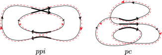
Figure 10: Two families of pairs of orbits differing in parallel encounters; both exist for systems with and without ${\cal T}$-invariance; each contributes to $\tau^{3}$, but the contributions mutually cancel. For labels see text.

III.1.3 Recursion relation for $N(\vec{v})$

We now derive a recursion formula for $N(\vec{v})$, imagining one loop (e.g. the one with index $L$) of an orbit removed and studying the consequences on the encounters. We shall reason with permutations but the translation rule cycle $\to$ encounter yields an interpretation for orbits. Readers wanting to skip the reasoning may jump to the result (44).

As a preparation, let us introduce a subset ${\cal M}(\vec{v},l)$ of ${\cal M}(\vec{v})$ such that the largest of the permuted numbers, i.e. $L(\vec{v})=\sum_{k}kv_{k}$ belongs to a cycle of length $l$ (it is assumed that $v_{l}>0$). The full set can be obtained by applying to this subset all $L(\vec{v})$ possible cyclic permutations. In fact, we thus get the set ${\cal M}(\vec{v})$ in $lv_{l}$ copies, since cyclic permutations shifting the element $L(\vec{v})$ inside an $l$-cycle or between different $l$-cycles with the same $l$ leave the subset ${\cal M}(\vec{v},l)$ unchanged. Consequently, the sizes of ${\cal M}(\vec{v})$ and ${\cal M}(\vec{v},l)$ are related as

$$N(\vec{v},l)=\frac{lv_{l}}{L(\vec{v})}N(\vec{v})\,.$$ (32)

We need a mapping that leads from a given permutation $P_{\rm enc}$ to a permutation $Q_{\rm enc}$ of smaller size, with a different cycle structure. Recall that any permutation $P_{\rm enc}\in{\cal M}(\vec{v},l)$ may be written as $P_{\rm enc}=P_{\rm loop}^{-1}P$, with $P_{\rm loop}$ the single-cycle permutation $(1,2,\ldots,L)$, and $P$ single-cycle as well. Now suppose that the element $L$ (corresponding to the entrance port following the $L$-th orbit loop) is deleted from the cycle representations of both $P_{\rm loop}$ and $P$. We thus obtain two new single-cycle permutations $Q_{\rm loop}$ and $Q$, acting on the numbers $1,2\ldots,L-1$. Here, $Q_{\rm loop}$ is simply given by $Q_{\rm loop}=(1,2,\ldots,L-1)$, and $Q$ differs from $P$ only by mapping the predecessor of $L$, i.e. $P^{-1}(L)$, to the successor of $L$, i.e. $P(L)$. Let us now define the new “encounter” permutation $Q_{\rm enc}$ in analogy to (31),

$$Q_{\rm enc}=Q_{\rm loop}^{-1}Q\,.$$ (33)

The $Q_{\rm enc}$ thus obtained acts on the elements $a=1,2,\ldots,L-1$ as

$$Q_{\rm enc}(a)=\begin{cases}P_{\rm enc}(L)&\text{if $a=P_{\rm enc}^{-1}(L-1)$}\\ L-1&\text{if $a=P_{\rm enc}^{-1}(L)$}\\ P_{\rm enc}(a)&\text{otherwise}\;.\end{cases}$$ (34)

To verify this, recall that $Q_{\rm loop}$ differs from $P_{\rm loop}$ only in the mapping of one number, same as for $Q$ and $P$. Thus $Q_{\rm enc}$ acts like $P_{\rm enc}$ on all but two numbers $a$. These exceptional cases, given in the first two lines of (34), are checked by carefully applying the above definitions of $Q_{\rm loop}$ and $Q$ as follows

$$Q_{\rm enc}P_{\rm enc}^{-1}(L-1) = Q_{\rm loop}^{-1}QP^{-1}P_{\rm loop}(L-1)$$

$$= Q_{\rm loop}^{-1}QP^{-1}(L)=Q_{\rm loop}^{-1}P(L)$$

$${\stackrel{{\scriptstyle(*)}}{{=}}} P_{\rm loop}^{-1}P(L)=P_{\rm enc}(L)$$

$$Q_{\rm enc}P_{\rm enc}^{-1}(L) = Q_{\rm loop}^{-1}QP^{-1}P_{\rm loop}(L)$$ (35)

$$= Q_{\rm loop}^{-1}QP^{-1}(1){\stackrel{{\scriptstyle(**)}}{{=}}}Q_{\rm loop}^{-1}PP^{-1}(1)$$

$$= Q_{\rm loop}^{-1}(1)=L-1\,;$$

here, we used $P(L)\neq 1$ for $(*)$, since otherwise $P_{\rm enc}$ would have a 1-cycle (i.e. $P_{\rm enc}(L)=P_{\rm loop}^{-1}P(L)=P_{\rm loop}^{-1}1=L$), and $P(L)\neq L$, since otherwise $P$ would have a 1-cycle. To check $(**)$, we need $P^{-1}(1)\neq L$ (since $P(L)\neq 1$) and $P^{-1}(1)\neq P^{-1}(L)$.

We need to connect the cycle structures of $Q_{\rm enc}$ and $P_{\rm enc}$. Let us first consider the case that the element $L-1$ of the permutation $P_{\rm enc}$ belongs to a different cycle than $L$, say a $k$-cycle. Hence, $P_{\rm enc}$ has the form

$$P_{\rm enc}=[\ldots](L-1,a_{2},a_{3},\ldots a_{k})(L,b_{2},b_{3},\ldots b_{l})$$ (36)

where the two aforementioned cycles are written in round brackets, and $[\ldots]$ stands for all other cycles. Then $Q_{\rm enc}$ differs from $P_{\rm enc}$ by mapping $P_{\rm enc}^{-1}(L-1)=a_{k}$ to $P_{\rm enc}(L)=b_{2}$, and $P_{\rm enc}^{-1}(L)=b_{l}$ to $L-1$. It follows that the $k$- and $l$-cycles of $P_{\rm enc}$ merge to a $(k+l-1)$-cycle of

$$Q_{\rm enc}=[\ldots](L-1,a_{2},a_{3},\ldots a_{k},b_{2},b_{3},\ldots b_{l})$$ (37)

where $[\ldots]$ is the same as in (36). Compared to $P_{\rm enc}$, $Q_{\rm enc}$ has one $k$-cycle and one $l$-cycle less, but one additional $(k+l-1)$-cycle. The changed cycle structure with $v_{k}\to v_{k}-1,v_{l}\to v_{l}-1,v_{k+l-1}\to v_{k+l-1}+1$ will be denoted as $\vec{v}^{\;[k,l\to k+l-1]}$. In general, $\vec{v}^{[\alpha_{1},\ldots,\alpha_{m}\to\beta_{1},\ldots,\beta_{n}]}$, $m\geq 0$, $n\geq 0$ denotes the vector obtained from $\vec{v}$ if we decrease all $v_{\alpha_{i}}$ by one, increase all $v_{\beta_{i}}$ by one, and leave all other components unchanged; if no $\beta_{i}$ appear on the r. h. s., no components of $\vec{v}$ are increased.

The permutation $Q_{\rm enc}$ thus belongs to the subset ${\cal M}(\vec{v}^{[k,l\to k+l-1]},k+l-1)$ since the largest permuted number $L-1$ belongs to a cycle with the length $k+l-1$. Each $P_{\rm enc}$ with the structure (36) ($k$ and $l$ fixed) generates one member of this subset. Vice versa, for fixed $k$ the $Q_{\rm enc}$ given in (37) uniquely determines one $P_{\rm enc}$ as given in (36). Hence, there are

$$N(\vec{v}^{[k,l\to k+l-1]},k+l-1)\,$$ (38)

members of ${\cal M}(\vec{v},l)$ structured like (36). Physically, the present scenario corresponds to the merger of a $k$- and an $l$-encounter into a $(k+l-1)$-encounter, by shrinking away an intervening loop.

We now turn to the second scenario where $L$ and $L-1$ belong to the same $l$-cycle of $P_{\rm enc}$. If $L$ follows $L-1$ after $m$ iterations (i.e. $L=P_{\rm enc}^{m}(L-1)$, $1\leq m\leq l-2$), the permutation $P_{\rm enc}$ is of the form

$$P_{\rm enc}=[\ldots](L-1,a_{2},a_{3},\ldots a_{m},L,a_{m+2},\ldots,a_{l})\,.$$ (39)

According to (34), $Q_{\rm enc}$ differs from $P_{\rm enc}$ by mapping $P_{\rm enc}^{-1}(L-1)=a_{l}$ to $P_{\rm enc}=a_{m+2}$ and mapping $P_{\rm enc}^{-1}(L)=a_{m}$ to $L-1$; $Q_{\rm enc}$ thus reads

$$Q_{\rm enc}=[\ldots](L-1,a_{2},a_{3},\ldots a_{m})(a_{m+2},\ldots,a_{l})\,;$$ (40)

the $l$-cycle of $P_{\rm enc}$ is broken up into 2 cycles, with the lengths $m$ and $l-m-1$. Since the largest number $L-1$ is included in an $m$-cycle, $Q_{\rm enc}$ belongs to ${\cal M}(\vec{v}^{[l\to m,l-m-1]},m)$.

In contrast to the first scenario, there are typically several $P_{\rm enc}$ producing the same $Q_{\rm enc}$. Indeed (40) would not only result from (39), but also from all $l-m-1$ permutations $P_{\rm enc}$ obtained by cyclic permutation of the last elements $a_{m+2},\ldots,a_{l}$ in (39). Besides, $[\ldots]$ in $P_{\rm enc}$ contains $v_{l-m-1}$ cycles of length $l-m-1$. If we transpose the content of one of these cycles with the subsequence $a_{m+2},\ldots,a_{l}$ in (39), the resulting $P_{\rm enc}$ will lead to the same $Q_{\rm enc}$. Thus, for each $m$, the subset of elements $P_{\rm enc}\in{\cal M}(\vec{v},l)$ structured like (39) is $(l-m-1)(v_{l-m-1}+1)$ times larger than ${\cal M}(\vec{v}^{[l\to m,l-m-1]},m)$, i.e. it has the size

$$(l-m-1)(v_{l-m-1}+1)N(\vec{v}^{[l\to m,l-m-1]},m)\,.$$ (41)

We have now decomposed ${\cal M}(\vec{v},l)$ into several subsets of size $N(\vec{v}^{[k,l\to k+l-1]},k+l-1)$, $k\geq 2$, and further subsets of size $(l-m-1)(v_{l-m-1}+1)N(\vec{v}^{[l\to m,l-m-1]},m)$, $m=1,\ldots,l-1$. The size of ${\cal M}(\vec{v},l)$ thus reads

$$N(\vec{v},l)=\sum_{k\geq 2}N(\vec{v}^{[k,l\to k+l-1]},k+l-1)$$ (42)

$$+\sum_{m=1}^{l-2}(l-m-1)(v_{l-m-1}+1)N(\vec{v}^{[l\to m,l-m-1]},m)\,.$$

We may rewrite the latter equation using $N(\vec{v},l)=\frac{lv_{l}}{L}N(\vec{v})$ and $\tilde{N}(\vec{v})=N(\vec{v})\frac{(-1)^{V}\prod_{l}l^{v_{l}}}{L(\vec{v})}$, to get

$$v_{l}\tilde{N}(\vec{v})+\sum_{k\geq 2}(v_{k+l-1}+1)k\tilde{N}(\vec{v}^{[k,l\to k+l-1]})$$

$$+\sum_{1\leq m\leq l-2}(v_{l-m-1}+1)v_{m}^{[l\to m,l-m-1]}\tilde{N}(\vec{v}^{[l\to m,l-m-1]})$$

$$=0\,;$$ (43)

Eqs. (42,III.1.3) are the general recursion relations in search. (Note that $v_{k+l-1}+1=v_{k+l-1}^{[k,l\to k+l-1]}$. Of course, the $k$th summand vanishes if there are no $k$-cycles present, i.e. if $v_{k}=0$ and thus formally $v_{k}^{[k,l\to k+l-1]}=-1$).

To determine the form factor for systems without time-reversal invariance, we only need the special case $l=2$. In this case, our recursion strongly simplifies,

$$v_{2}\tilde{N}(\vec{v})+\sum_{k\geq 2}v_{k+1}^{[k,2\to k+1]}k\tilde{N}(\vec{v}^{[k,2\to k+1]})=0\,,$$ (44)

since only the first of the two above scenarios is possible. That is, a 2-cycle may only merge with a $k$-cycle to form a $(k+1)$-cycle, but not split into two separate cycles. Recall that $\vec{v}^{[k,2\to k+1]}$ is obtained from $\vec{v}$ by decreasing both $v_{k}$ and $v_{2}$ by one, and increasing $v_{k+1}$ by one.

III.1.4 Spectral form factor

We had expressed the Taylor coefficients of the form factor as a sum over the combinatorial numbers $\tilde{N}(\vec{v})$,

$$K_{n}=\frac{1}{(n-2)!}\sum_{\vec{v}}^{\nu(\vec{v})=n}\tilde{N}(\vec{v})\,,\quad n\geq 2\,,$$ (45)

see (29), where the sum runs over all $\vec{v}$ with $v_{1}=0$ which fulfill $\nu(\vec{v})\equiv L(\vec{v})-V(\vec{v})+1=n$. Our recursion relation for $\tilde{N}(\vec{v})$ now translates into one for $K_{n}$, albeit a trivial one in the unitary case, implying that all $K_{n}$ except $K_{1}$ vanish. (Alternatively, one may use a rather involved explicit formula for $N(\vec{v})$ JMueller .)

To show this, consider the recursion (44) for $\tilde{N}(\vec{v})$ and sum over $\vec{v}$ as above

$$\sum_{\vec{v}}^{\nu(\vec{v})=n}\left(v_{2}\tilde{N}(\vec{v})+\sum_{k\geq 2}v_{k+1}^{[k,2\to k+1]}k\tilde{N}(\vec{v}^{[k,2\to k+1]})\right)=0\,.$$ (46)

Each of the sums $\sum_{\vec{v}}^{\nu(\vec{v})=n}v_{k+1}^{[k,2\to k+1]}\tilde{N}(\vec{v}^{[k,2\to k+1]})$ may be transformed into a sum over the argument of $\tilde{N}$, i.e. $\vec{v}^{\prime}=\vec{v}^{[k,2\to k+1]}$. Due to $\nu(\vec{v})=n$, we also have $\nu(\vec{v}^{\prime})=n$, since going from $\vec{v}$ to $\vec{v}^{\prime}$ decreases both $L$ and $V$ by one and thus leaves $\nu$ invariant. Given that by construction we must have $v^{\prime}_{k+1}\geq 1$, the sum over $\vec{v}^{\prime}$ extends over all $\vec{v}^{\prime}$ with $\nu(\vec{v}^{\prime})=n$ and $v^{\prime}_{k+1}\geq 1$. However, the latter restriction may be dropped because due to the prefactor $v^{\prime}_{k+1}$ terms with $v^{\prime}_{k+1}=0$ do not contribute. Consequently, the sum may be simplified as

$$\sum_{\vec{v}}^{\nu(\vec{v})=n}v_{k+1}^{[k,2\to k+1]}\tilde{N}(\vec{v}^{[k,2\to k+1]})=\sum_{\vec{v}^{\prime}}^{\nu(\vec{v}^{\prime})=n}v^{\prime}_{k+1}\tilde{N}(\vec{v}^{\prime})\,.$$ (47)

Applying this rule to all terms in (46) and dropping the primes, we obtain

$$\sum_{\vec{v}}^{\nu(\vec{v})=n}\Big{(}v_{2}+\sum_{k\geq 2}v_{k+1}k\Big{)}\tilde{N}(\vec{v})=0\,.$$ (48)

Since the term in brackets is just $\sum_{l\geq 2}v_{l}(l-1)=L-V=n-1$ we have

$$(n-1)\sum_{\vec{v}}^{\nu(\vec{v})=n}\tilde{N}(\vec{v})=(n-1)!\,K_{n}=0\,,\quad n\geq 2\,.$$ (49)

We see that all Taylor coefficients except $K_{1}$ vanish: orbit pairs differing in encounters yield no net contribution; the diagonal approximation exhausts the small-time form factor in full. GUE behavior is thus ascertained.

III.2 Orthogonal case

III.2.1 Structures and permutations

In $\cal T$-invariant systems the partners of an orbit $\gamma$ may involve loops of both $\gamma$ and its time-reversed $\overline{\gamma}$. To capture all partners $\gamma^{\prime}$ of $\gamma$ in terms of permutations the permuted objects must refer to both $\gamma$ and $\overline{\gamma}$ and thus be doubled in number compared to the unitary case. Each permutation will describe simultaneously both $\gamma^{\prime}$ and $\bar{\gamma}^{\prime}$.

We number the entrance and exit ports of self-encounters of $\gamma$ in their order of traversal, $1,2,\ldots,L$, such that the $a$-th encounter stretch leads from the $a$-th entrance to the $a$-th exit port; see Fig. 11 for the example of a 2-encounter. The time-reversed orbit $\overline{\gamma}$ passes the same ports as $\gamma$, but with opposite sense and entrance and exit swapped. The ports of $\overline{\gamma}$ are labelled by $\overline{1},\overline{2},\ldots,\overline{L}$, such that the exit port $\overline{a}$ of $\overline{\gamma}$ is the time-reversed of the entrance port $a$ of $\gamma$, and entrance port $\overline{a}$ of $\overline{\gamma}$ is the time-reversed of the exit port $a$ of $\gamma$, again compare Fig. 11. Consequently, inside $\overline{\gamma}$ stretch $\overline{a}$ leads from entrance $\overline{a}$ to exit $\overline{a}$.

The intra-encounter connections of $\gamma$ and $\overline{\gamma}$ are represented by the trivial permutation $P_{\rm enc}^{\gamma}=\left({1\atop 1}{2\atop 2}{\ldots\atop\ldots}{L\atop L}{\overline{1}\atop\overline{1}}{\overline{2}\atop\overline{2}}{\ldots\atop\ldots}{\overline{L}\atop\overline{L}}\right)$ which maps each entrance (upper line) to the following exit (lower line). The loops are associated with $P_{\rm loop}=\left({1\atop 2}{2\atop 3}{\ldots\atop\ldots}{L\atop 1}{\overline{2}\atop\overline{1}}{\overline{3}\atop\overline{2}}{\ldots\atop\ldots}{\overline{1}\atop\overline{L}}\right)$, since if one loop of $\gamma$ leads from the exit of the $(a-1)$-st stretch to the entrance of the $a$-th one, its time-reversed must go from exit $\overline{a}$ to entrance $\overline{a-1}$. Finally, $P^{\gamma}=P_{\rm loop}P_{\rm enc}^{\gamma}=P_{\rm loop}$ specifies the ordering of entrance ports along $\gamma$ and $\overline{\gamma}$. That $P^{\gamma}$ has two cycles $(1,2,\ldots,L)$ and $(\overline{L},\overline{L-1},\ldots,\overline{1})$, one each for $\gamma$ and $\overline{\gamma}$.

The reconnections leading to $\gamma^{\prime}$, $\overline{\gamma^{\prime}}$ are described by a permutation $P_{\rm enc}$ determining the exit port connected to each entrance. In the example of a Sieber/Richter pair, Fig. 11, the partner $\gamma^{\prime}$ connects the entrance 1 of $\gamma$ to the exit $\bar{2}$ of $\bar{\gamma}$, and the entrance $\bar{1}$ of $\bar{\gamma}$ to the exit 2 of $\gamma$. Including the connections in the time-reversed partner $\bar{\gamma^{\prime}}$, we write $P_{\rm enc}=\left({1\atop\overline{2}}{2\atop\overline{1}}{\overline{1}\atop 2}{\overline{2}\atop 1}\right)$. Note that the sequence of columns in $P_{\rm enc}$ may be ordered arbitrarily. We shall mostly order such that the first lines in $P_{\rm enc}$ and $P_{\rm enc}^{\gamma}$ coincide; columns describing $\gamma^{\prime}$ and $\overline{\gamma^{\prime}}$ may thus become mutually interspersed.

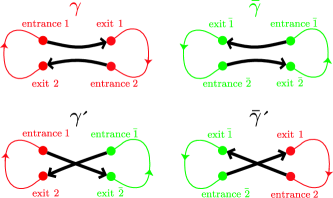
Figure 11: Entrance-to-exit connections for a Sieber/Richter pair, in an orbit $\gamma$, its time-reversed $\bar{\gamma}$, and the partners $\gamma^{\prime},\bar{\gamma^{\prime}}$.

$\cal T$-invariance imposes a restriction on $P_{\rm enc}$: If a stretch connects entrance $a$ to exit $b$, the time-reversed stretch must connect the entrance $\overline{b}$ of $\overline{\gamma}$ to the exit $\overline{a}$. Thus, if $P_{\rm enc}$ maps $a$ to $b$, it has to map $\overline{b}$ to $\overline{a}$, with $a,b$ standing for elements out of $1,\ldots,L,\bar{1},\ldots,\bar{L}$ (we define $\overline{\overline{a}}=a$). This restriction on $P_{\rm enc}$ will be referred to as “$\cal T$-covariance”.

It follows that if $(a_{1},a_{2},\ldots,a_{l-1},a_{l})$ is a cycle of $P_{\rm enc}$, then so is its “time-reversed” , $(\overline{a_{l}},\overline{a_{l-1}},\ldots,\overline{a_{2}},\overline{a_{1}})$. These two cycles may not be identical. Indeed a cycle coinciding with its time-reversed would have the form $\left(a_{1},\ldots,a_{k},\overline{a_{k}},\ldots,\overline{a_{1}}\right),\;k=l/2$; such cycles are not allowed, since the entrance port $a_{k}$ and the exit port $\bar{a}_{k}$ coincide in configuration space and thus may not be connected by an encounter stretch.

We see that given time reversal there must be a pair of twin $l$-cycles of $P_{\rm enc}$ associated with each $l$-encounter; an encounter associated with more than one pair of cycles would decompose into several independent ones. In general, each cycle in a pair describes stretches both of $\gamma^{\prime}$ and of $\bar{\gamma}^{\prime}$; only in case of all stretches nearly parallel one cycle refers exclusively to $\gamma^{\prime}$ and the other to $\overline{\gamma^{\prime}}$.

The final restriction on the permutations $P_{\rm enc}$ is analogous to the one encountered in the unitary case. To obtain two connected partner orbits $\gamma^{\prime}$ and $\overline{\gamma^{\prime}}$, we now have to demand the permutation $P=P_{\rm loop}P_{\rm enc}$ to consist of only two $L$-cycles, listing the entrance ports in $\gamma^{\prime}$ and $\overline{\gamma^{\prime}}$, respectively. (The second cycle can also be interpreted as the list of exit ports of $\gamma^{\prime}$, time reversed and written in reverse order. Since an entrance $a_{i}$ is connected by a loop to the exit $b_{i}\equiv P_{\rm loop}^{-1}(a_{i})$, the two cycles of $P$ read $(a_{1},a_{2},\ldots,a_{L})$ and $(\overline{b_{L}},\overline{b_{L-1}},\ldots,\overline{b_{1}})$.)

To summarize, we consider the set ${\cal M}(\vec{v})$ of permutations $P_{\rm enc}$ acting on $1,2,\ldots,L,\overline{1},\overline{2},\ldots,\overline{L}$ which (i) are time-reversal covariant, (ii) have $v_{l}$ pairs of $l$-cycles for all $l\geq 2$, and (iii) lead to a permutation $P=P_{\rm loop}P_{\rm enc}$ consisting of two cycles as above. Each element $P_{\rm enc}$ of the set ${\cal M}(\vec{v})$ thus stands for one of the “structures” introduced in II.4. We need to calculate the number $N(\vec{v})$ of elements of ${\cal M}(\vec{v})$.

III.2.2 Examples

order	$\vec{v}$	$L$	$V$	$N(\vec{v})$	$\tilde{N}(\vec{v})$	contribution
$\tau^{2}$	$(2)^{1}$	2	1	1	$-1$	$-2\tau^{2}$
					$-1$	$-2\tau^{2}$
$\tau^{3}$	$(2)^{2}$	4	2	5	5	$10\tau^{3}$
	$(3)^{1}$	3	1	4	$-4$	$-8\tau^{3}$
					1	2$\tau^{3}$
$\tau^{4}$	$(2)^{3}$	6	3	41	$-\frac{164}{3}$	$-\frac{164}{3}\tau^{4}$
	$(2)^{1}(3)^{1}$	5	2	60	72	$72\tau^{4}$
	$(4)^{1}$	4	1	20	$-20$	$-20\tau^{4}$
					$-\frac{8}{3}$	$-\frac{8}{3}\tau^{4}$
$\tau^{5}$	$(2)^{4}$	8	4	509	1018	$\frac{1018}{3}\tau^{5}$
	$(2)^{2}(3)^{1}$	7	3	1092	$-1872$	$-624\tau^{5}$
	$(2)^{1}(4)^{1}$	6	2	504	672	$224\tau^{5}$
	$(3)^{2}$	6	2	228	342	$114\tau^{5}$
	$(5)^{1}$	5	1	148	$-148$	$-\frac{148}{3}\tau^{5}$
					12	4$\tau^{5}$

Table 2: Permutations, and thus families of orbit pairs, giving rise to orders $\tau^{2}$ to $\tau^{5}$ of the form factor, for systems with ${\cal T}$-invariance; notation as in Table 1. The results coincide with the predictions of RMT for the GOE.

Again, the numbers $N(\vec{v})$ can be determined by numerically counting permutations. From the results shown in Table 2, we see that indeed the form factor of the Gaussian Orthogonal Ensemble is reproduced semiclassically.

The $\tau^{2}$ contribution comes from pairs of orbits differing in one antiparallel 2-encounter SR . We have already shown that the corresponding “encounter permutation” reads $P_{\rm enc}=\left({1\atop\overline{2}}{2\atop\overline{1}}{\overline{1}\atop 2}{\overline{2}\atop 1}\right)$.

The $\tau^{3}$ contribution originates from (compare Figs. 10, 12 and Ref. Tau3 ) four permutations related to 3-encounters and five permutations related to pairs of 2-encounters. The permutation $P_{\rm enc}=\left({1\atop 2}{2\atop 3}{3\atop 1}{\overline{1}\atop\overline{3}}{\overline{2}\atop\overline{1}}{\overline{3}\atop\overline{2}}\right)$ describes encounters of three parallel orbit stretches $\mathrel{\,\lower 0.6458pt\hbox{\begin{picture}(4.0,3.0)\put(0.0,0.3){\vector(1,0){4.0}}\put(0.0,1.5){\vector(1,0){4.0}} \put(0.0,2.7){\vector(1,0){4.0}} \end{picture}}\,}$ (case pc). For triple encounters in which one of the stretches is time-reversed with respect to the other two $\mathrel{\,\lower 0.6458pt\hbox{\begin{picture}(4.0,3.0)\put(4.0,0.3){\vector(-1,0){4.0}}\put(0.0,1.5){\vector(1,0){4.0}} \put(0.0,2.7){\vector(1,0){4.0}} \end{picture}}\,}$ (case ac), there are three related permutations, $P_{\rm enc}=\left({1\atop\overline{3}}{2\atop 3}{3\atop\overline{1}}{\overline{1}\atop 2}{\overline{2}\atop 1}{\overline{3}\atop\overline{2}}\right)$ and its two images under cyclic permutation of 1,2,3 as well as $\overline{1},\overline{2},\overline{3}$; physically, the three latter are equivalent since they differ only in which of the three stretches is considered the first. (In Ref. Tau3 such equivalences were taken into account by multiplicity factors ${\cal N}_{pc}$ and ${\cal N}_{ac}$.)

Pairs of 2-encounters may either be composed of either (i) two parallel encounters ($P_{\rm enc}=\left({1\atop 3}{2\atop 4}{3\atop 1}{4\atop 2}{\overline{1}\atop\overline{3}}{\overline{2}\atop\overline{4}}{\overline{3}\atop\overline{1}}{\overline{4}\atop\overline{2}}\right)$, family ppi) or (ii) one parallel and one antiparallel encounter ($P_{\rm enc}=\left({1\atop\overline{3}}{2\atop 4}{3\atop\overline{1}}{4\atop 2}{\overline{1}\atop 3}{\overline{2}\atop\overline{4}}{\overline{3}\atop 1}{\overline{4}\atop\overline{2}}\right)$ and $P_{\rm enc}=\left({1\atop 3}{2\atop\overline{4}}{3\atop 1}{4\atop\overline{2}}{\overline{1}\atop\overline{3}}{\overline{2}\atop 4}{\overline{3}\atop\overline{1}}{\overline{4}\atop 2}\right)$, family api), or (iii) two antiparallel ones ($P_{\rm enc}=\left({1\atop\overline{4}}{2\atop\overline{3}}{3\atop\overline{2}}{4\atop\overline{1}}{\overline{1}\atop 4}{\overline{2}\atop 3}{\overline{3}\atop 2}{\overline{4}\atop 1}\right)$ and $P_{\rm enc}=\left({1\atop\overline{2}}{2\atop\overline{1}}{3\atop\overline{4}}{4\atop\overline{3}}{\overline{1}\atop 2}{\overline{2}\atop 1}{\overline{3}\atop 4}{\overline{4}\atop 3}\right)$, family aas in Tau3 ). Again, equivalent permutations differ by cyclic permutations (of now 1,2,3,4 as well as $\overline{1},\overline{2},\overline{3},\overline{4}$), i.e. in which of the stretches is assigned the number 1.

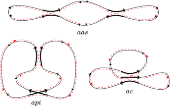
Figure 12: Pairs of orbits existing only for systems with ${\cal T}$-invariance and giving all of $\tau^{3}$. For labels see text. Two further families do not require ${\cal T}$-invariance, see Fig. 10.

III.2.3 Recursion relation for $N(\vec{v})$

We are now fully equipped to establish a recursion relation for $N(\vec{v})$ in much the same way in the unitary case. Impatient readers may want to jump to the resulting recursion (68) for $K_{n}$.

First of all, we recover Eq. (32), $N(\vec{v},l)=\frac{v_{l}l}{L}N(\vec{v})$ using exactly the same arguments as in the unitary case. From each element $P_{\rm enc}\in{\cal M}(\vec{v},l)$ we obtain $L$ elements of ${\cal M}(\vec{v})$ by the $L$ possible cyclic permutations. Applying these cyclic permutations to the set ${\cal M}(\vec{v},l)$ we obtain $v_{l}l$ copies of ${\cal M}(\vec{v})$, since the $v_{l}$ pairs of twin $l$-cycles have altogether $v_{l}l$ members without overbar, and permutations shifting $L$ among these members leave ${\cal M}(\vec{v},l)$ invariant.

Choosing a permutation $P_{\rm enc}=P_{\rm loop}^{-1}P\in{\cal M}(\vec{v},l)$ we set $Q_{\rm enc}=Q_{\rm loop}^{-1}Q$ with $Q_{\rm loop}$ and $Q$ obtained from $P_{\rm loop}$ and $P$ by omitting $L$ and $\overline{L-1}$, and replacing $\overline{L}$ by $\overline{L-1}$. (This prescription can be interpreted as removing the loop leading from exit $L-1$ to entrance $L$, and its time-reversed leading from exit $\overline{L}$ to entrance $\overline{L-1}$; hence the corresponding entrance ports must be removed from $P$ and $P_{\rm loop}=P^{\gamma}$.) In particular $Q_{\rm loop}$ will have the form $Q_{\rm loop}=(1,2,\ldots,L-1)(\overline{L-1},\overline{L-2},\ldots,\overline{1})$. The two cycles of $Q$ fulfill the same relation as those of $P$ and may thus indeed be interpreted as lists of entrance ports of two time reversed orbits. The resulting “encounter permutation” $Q_{\rm enc}$ maps the remaining elements $a=1,2,\ldots,L-1,\overline{1},\overline{2},\ldots,\overline{L-1}$ as

$$Q_{\rm enc}(a)=\begin{cases}P_{\rm enc}(L)&\text{if $a=P_{\rm enc}^{-1}(L-1)$}\\ P_{\rm enc}(\overline{L-1})&\text{if $a=P_{\rm enc}^{-1}(\overline{L})$}\\ L-1&\text{if $a=P_{\rm enc}^{-1}(L)$}\\ P_{\rm enc}(\overline{L})&\text{if $a=\overline{L-1}$}\\ P_{\rm enc}(a)&\text{otherwise}\,.\end{cases}$$ (50)

Here, the second and fourth line extend (34) as required by ${\cal T}$ invariance; the present $Q_{\rm enc}$ is indeed ${\cal T}$ covariant.

When analyzing the cycle structure of $Q_{\rm enc}$, we now have to distinguish three cases, the first two paralleling the treatment of III.1.3. Note however a factor 2 appearing in the second case. For each $Q_{\rm enc}\in{\cal M}(\vec{v}^{[l\to m,l-m-1]},m)$, there are now twice as many, namely $2(l-m-1)(v_{l-m-1}+1)$ related $P_{\rm enc}\in{\cal M}(\vec{v},l)$ structured like (39), since $Q_{\rm enc}$ also remains unaffected by time reversal of $a_{m+2},\ldots,a_{l}$ in (39). The second and fourth line in (50) make sure that merging or splitting of cycles is mirrored by the respective twins.

A third possibility appears since the cycles involving $L$ and $L-1$ may be twins, and hence belong to the same encounter. Since the twin cycles are mutually time reversed there is one cycle containing both $L$ and $\overline{L-1}$, and another one containing $\overline{L}$ and $L-1$. Assume that inside the first cycle, the element $\overline{L-1}$ follows $L$ after $m$ iterations, i.e. $\overline{L-1}=P_{\rm enc}^{m}(L)$ (with $1\leq m\leq l-1$). Then $P_{\rm enc}$ can be written as

$$P_{\rm enc}= [\ldots](L,a_{2},\ldots,a_{m},\overline{L-1},a_{m+2},\ldots,a_{l})$$ (51)

$$(\overline{a_{l}},\ldots,\overline{a_{m+2}},L-1,\overline{a_{m}},\ldots,\overline{a_{2}},\overline{L})\,.$$

Due to (50), $Q_{\rm enc}$ differs from $P_{\rm enc}$ by mapping

$$Q_{\rm enc}(\overline{a_{m+2}})=a_{2}\quad\quad\quad Q_{\rm enc}(\overline{a_{2}})=a_{m+2}$$

$$Q_{\rm enc}(a_{l})=L-1\quad\quad\quad Q_{\rm enc}(\overline{L-1})=\overline{a_{l}}$$ (52)

The initial pair of twin cycles of $P_{\rm enc}$ is transformed to the following pair of twin $(l-1)$-cycles of

$$Q_{\rm enc}= [\ldots](a_{2},\ldots,a_{m},\overline{L-1},\overline{a_{l}},\ldots,\overline{a_{m+2}})$$ (53)

$$(a_{m+2},\ldots,a_{l},L-1,\overline{a_{m}},\ldots,\overline{a_{2}})\,.$$

Given that the largest number permuted by $Q_{\rm enc}$, i.e. $L-1$, is included in one of these cycles, we have $Q_{\rm enc}\in{\cal M}(\vec{v}^{[l\to l-1]},l-1)$. Conversely, for any such $Q_{\rm enc}$ and each $1\leq m\leq l-1$, there is exactly one related $P_{\rm enc}$, since we may read off $a_{2},\ldots,a_{l}$ from $Q_{\rm enc}$ in (53) and recombine them to form a permutation $P_{\rm enc}$ as in (51). We thus see that each of the $l-1$ subsets of ${\cal M}(\vec{v},l)$ with $\overline{L-1}=P_{\rm enc}^{m}(L)$ is one-to-one to ${\cal M}(\vec{v}^{[l\to l-1]},l-1)$ and thus has an equal number of elements.

We have seen that ${\cal M}(\vec{v},l)$ falls into subsets similar to the unitary case, time-reversal invariance making for the factor 2 explained above, and for $l-1$ additional subsets of size $N(\vec{v}^{[l\to l-1]},l-1)$. The various sizes combine to the orthogonal analogue of the recursion relation (42),

$$N(\vec{v},l)=\sum_{k\geq 2}N(\vec{v}^{[k,l\to k+l-1]},k+l-1)$$

$$+\sum_{m=1}^{l-2}2(l-m-1)(v_{l-m-1}+1)N(\vec{v}^{[l\to m,l-m-1]},m)$$

$$+(l-1)N(\vec{v}^{[l\to l-1]},l-1)\,,$$ (54)

which using (32) and the shorthand $\tilde{N}(\vec{v})=N(\vec{v})\frac{(-1)^{V}\prod_{l}l^{v_{l}}}{L}$ may be written as

$$v_{l}\tilde{N}(\vec{v})+\sum_{k\geq 2}(v_{k+l-1}+1)k\tilde{N}(\vec{v}^{[k,l\to k+l-1]})$$

$$+\sum_{m=1}^{l-2}2(v_{l-m-1}+1)v_{m}^{[l\to m,l-m-1]}\tilde{N}(\vec{v}^{[l\to m,l-m-1]})$$

$$-(l-1)(v_{l-1}+1)\tilde{N}(\vec{v}^{[l\to l-1]})=0\,;$$ (55)

recall that $v_{k+l-1}+1=v_{k+l-1}^{[k,l\to k+l-1]}$.

III.2.4 Spectral form factor

Similarly as in III.1.4 we now turn the recursion relation for $\tilde{N}(\vec{v})$ into one for the Taylor coefficients $K_{n}$. As a preparation we generalize our rule (47). For all similar sums over $\vec{v}$ with fixed $\nu(\vec{v})=n$ and $v_{1}=0$ we find

$$\sum_{\vec{v}}^{\nu(\vec{v})=n}\!\!f(\vec{v}^{[\alpha_{1},\alpha_{2},\ldots\to\beta]})\tilde{N}(\vec{v}^{[\alpha_{1},\alpha_{2},\ldots\to\beta]})=\!\!\!\!\sum_{\vec{v}^{\prime}}^{\nu(\vec{v}^{\prime})=n^{\prime}}\!\!\!f(\vec{v}^{\prime})\tilde{N}(\vec{v}^{\prime})\,,$$ (56)

with integers $\alpha_{i}\geq 2$, $\beta\geq 2$, $n^{\prime}=\nu(\vec{v}^{\prime})=\nu(\vec{v}^{[\alpha_{1},\alpha_{2},\ldots\to\beta]})=n-\sum_{i}(\alpha_{i}-1)+(\beta-1)$, and $f$ any function of $\vec{v}^{\prime}$ vanishing for $v^{\prime}_{\beta}=0$. Eq. (56) follows in the same way as (47), i.e. by switching to $\vec{v}^{\prime}=\vec{v}^{[\alpha_{1},\alpha_{2},\ldots\to\beta]}$ as the new summation variable and dropping the restriction $v^{\prime}_{\beta}\geq 1$ ($\vec{v}^{\prime}$ with $v^{\prime}_{\beta}=0$ do not contribute due to the vanishing of $f$). One similarly shows that the foregoing rule holds even without any conditions on $f$ if $\beta$ is removed, i.e. if no new cycles are created. It is convenient to abbreviate the r. h. s. of (56) with the help of

$$S_{n^{\prime}}[f]\equiv\sum_{\vec{v}^{\prime}}^{\nu(\vec{v}^{\prime})=n^{\prime}}f(\vec{v}^{\prime})\tilde{N}(\vec{v}^{\prime})\,$$ (57)

for arbitrary $f$; we note that $K_{n}=\frac{2}{(n-2)!}S_{n}[1]$. Thus equipped we turn to the three special cases $l=1,2,3$ of our recursion relations (III.2.3,III.2.3) which we shall need below.

First, the case $l=1$ involves permutations with 1-cycles, appearing only in intermediate steps of our calculation. If the element $L$ forms a 1-cycle, it may simply be removed from a permutation without affecting the other cycles, which corresponds to a transition $\vec{v}\to\vec{v}^{[1\to]}$. We thus have $N(\vec{v},1)=N(\vec{v}^{[1\to]})$ and equivalently

$$v_{1}\tilde{N}(\vec{v})+L(\vec{v}^{[1\to]})\tilde{N}(\vec{v}^{[1\to]})=0\,.$$ (58)

Second, for $l=2$ (and $v_{1}=0$) the recursion (III.2.3) boils down to

$$v_{2}\tilde{N}(\vec{v})+\sum_{k\geq 2}\left(v_{k+1}^{[k,2\to k+1])}k\tilde{N}(\vec{v}^{[k,2\to k+1]})\right)$$

$$-\tilde{N}(\vec{v}^{[2\to 1]})=0\,,$$ (59)

where only the last term is new compared to the unitary case. We bring it to a form free from 1-cycles by invoking (58) and thus $\tilde{N}(\vec{v}^{[2\to 1]})=-L(\vec{v}^{[2\to]})\tilde{N}(\vec{v}^{[2\to]})$, to get

$$v_{2}\tilde{N}(\vec{v})+\sum_{k\geq 2}\left(v_{k+1}^{[k,2\to k+1])}k\tilde{N}(\vec{v}^{[k,2\to k+1]})\right)$$

$$+L(\vec{v}^{[2\to]})\tilde{N}(\vec{v}^{[2\to]})=0\,.$$ (60)

As in the unitary case, we sum over all $\vec{v}$ with $v_{1}=0$ and $\nu(\vec{v})=n$. The rule (56) and the shorthand (57) give

$$S_{n}\Bigg{[}v_{2}+\sum_{k\geq 2}v_{k+1}k\Bigg{]}+S_{n-1}[L(\vec{v})]$$

$$=(n-1)S_{n}[1]+S_{n-1}[L(\vec{v})]=0\,.$$ (61)

A further relation is obtained by multiplying (III.2.4) with $L(\vec{v})-1=L(\vec{v}^{[k,2\to k+1]})=L(\vec{v}^{[2\to]})+1$ and again summing over $\vec{v}$ with the help of (56). The resulting equation

$$(n-1)S_{n}[L(\vec{v})]-S_{n}[v_{2}]+S_{n-1}[L(\vec{v})(L(\vec{v})+1)]=0$$ (62)

can be simplified by (III.2.4) and replacing $n\to n-2$,

$$-(n-2)(n-3)S_{n-1}[1]=S_{n-2}[v_{2}]-S_{n-3}[L(\vec{v})(L(\vec{v})+1)]\,.$$ (63)

Finally, we consider $l=3$ (and $v_{1}=0$)

$$v_{3}\tilde{N}(\vec{v})+\sum_{k\geq 2}\left(v_{k+2}^{[k,3\to k+2]}k\tilde{N}(\vec{v}^{[k,3\to k+2]})\right)$$

$$+4\tilde{N}(\vec{v}^{[3\to 1,1]})-2v_{2}^{[3\to 2]}\tilde{N}(\vec{v}^{[3\to 2]})=0\,.$$ (64)

The 1-cycles in the third term are eliminated using the identity $\tilde{N}(\vec{v}^{[3\to 1,1]})=\frac{1}{2}L(\vec{v}^{[3\to]})(L(\vec{v}^{[3\to]})+1)\tilde{N}(\vec{v}^{[3\to]})$, which follows by twice applying (58) to $\vec{v}^{[3\to 1,1]}$. Summing over $\vec{v}$ in (III.2.4) we find

$$S_{n}\Bigg{[}v_{3}+\sum_{k\geq 2}v_{k+2}k\Bigg{]}+2S_{n-2}[L(\vec{v})(L(\vec{v})+1)]$$

$$-2S_{n-1}[v_{2}]=0\,.$$ (65)

This expression can be simplified using $v_{3}+\sum_{k\geq 2}v_{k+2}k=\sum_{k\geq 2}v_{k}(k-2)=L(\vec{v})-2V(\vec{v})=2(\nu(\vec{v})-1)-L(\vec{v})$, i.e.

$$2(n-1)S_{n}[1]-S_{n}[L(\vec{v})]+2S_{n-2}[L(\vec{v})(L(\vec{v})+1)]$$

$$-2S_{n-1}[v_{2}]=0\,.$$ (66)

Finally applying (III.2.4), substituting $n\to n-1$, and dividing by 2, we proceed to

$$\frac{n-1}{2}S_{n}[1]+(n-2)S_{n-1}[1]$$

$$=S_{n-2}[v_{2}]-S_{n-3}[L(\vec{v})(L(\vec{v})+1)]\,.$$ (67)

Upon comparing the recursion relations (63) and (III.2.4), obtained for the cases $l=2$ and $l=3$, we find the coefficients $S_{n}[1]=\frac{(n-2)!}{2}K_{n}$ and $S_{n-1}[1]=\frac{(n-3)!}{2}K_{n-1}$ related as $\frac{n-1}{2}S_{n}[1]=-(n-2)^{2}S_{n-1}[1]$ or

$$(n-1)K_{n}=-2(n-2)K_{n-1}\,.$$ (68)

An initial condition is provided by the Sieber/Richter result for orbits differing in one 2-encounter, $K_{2}=-2$. Thus started, our recursion yields the Taylor coefficients

$$K_{n}=\frac{(-2)^{n-1}}{n-1}$$ (69)

coinciding with the random-matrix result. Universal behavior is thus ascertained for the small-time form factor of fully chaotic dynamics from the orthogonal symmetry class; the resulting series converges for $\tau<\frac{1}{2}$.

IV Spinning particles and the symplectic symmetry class

We now allow for a spin with arbitrary but fixed spin quantum number $S$. Assuming time-reversal invariance we know that for integer $S$ the time reversal operator ${\cal T}$ squares to unity, ${\cal T}^{2}=1$, whereas for half-integer spin, ${\cal T}^{2}=-1$; we face the orthogonal and symplectic symmetry class, respectively. The semiclassical theory of spinning particles is discussed in Keppeler ; off-diagonal terms of the form factor were considered in a preliminary version in Heusler , and for quantum graphs in BolteHarrison .

The Pauli Hamiltonian reads $H=H_{0}+\mathbf{\mathbf{\hat{B}}\cdot\hat{S}}$ where $\mathbf{\hat{S}}$ is the spin operator, with $\mathbf{\hat{S}}^{2}=\hbar^{2}S(S+1)$. The vector operator $\mathbf{\hat{B}}(\mathbf{\hat{q}},\mathbf{\hat{p}})$ describes the influence of the translational motion and external fields on the spin. The spin-orbit interaction formally behaves like $\cal{O}(\hbar)$ and tends to zero in the semiclassical limit; it is not a small quantum perturbation though, since its matrix elements are infinitely larger than the energy spacing $\Delta\sim{\cal O}(\hbar^{f}),\quad f>1$.

The state of the system is given by a spinor with $2S+1$ components and the propagator by a $(2S+1)\times(2S+1)$ matrix. In the leading order of the semiclassical approximation the propagator consists of the scalar translational part which is the van Vleck propagator of the spinless system, multiplied by the spin evolution matrix $d$ (belonging to the spin-$S$ representation $D^{(S)}$ of $SU(2)$); the latter matrix has to be evaluated on the classical orbit (of the translational motion) connecting the initial and final point. Along such an orbit $\gamma$ the $d$-matrix is a function of the initial and final times, $d=d_{\gamma}(t,t_{0})$. It satisfies the equation ${{\rm i}}\partial_{t}d_{\gamma}(t,t_{0})=\mathbf{B}_{\gamma}(t)\cdot(\mathbf{\hat{S}}/\hbar)\;d_{\gamma}(t,t_{0})$ where the classical time-dependent vector $\mathbf{B}_{\gamma}(t)$ is obtained by substituting the classical coordinates and momenta along $\gamma$ for the operator valued arguments of $\mathbf{\hat{B}}(\mathbf{\hat{q}},\mathbf{\hat{p}})$; the initial condition is $d_{\gamma}(t_{0},t_{0})=\mathbf{1}_{2S+1}$. Such semiclassical treatment keeps the translational motion unaffected by the quantum spin. The spin, however, is driven by the translational motion. No semiclassical approximation for the spin itself (which would require the assumption of large $S$) is invoked.

The full quantum nature of the spin (finite $S$) notwithstanding, a seemingly classical manner of speaking about the spin is possible, due to the following fact: any matrix from $D^{(S)}$ can be parametrized by three Euler angles (e.g. like $d(\theta,\phi,\psi)={\rm e}^{{{\rm i}}\psi\hat{S}_{z}/\hbar}{\rm e}^{{{\rm i}}\theta\hat{S}_{x}/\hbar}{\rm e}^{{{\rm i}}\phi\hat{S}_{z}/\hbar}$), which are time-dependent for $d=d(t)$. The angles $\psi(t),\theta(t),\phi(t)$ may also be imagined to specify the orientation of a fictitious rigid body in classical rotation; as done in Keppeler ; Heusler ; BolteHarrison we shall speak of that motion as “spin rotation”.

We assume the translational motion chaotic as before and require ergodicity of the combined spin rotation and translational motion. The spin rotation itself is then also ergodic. This means that time averages of the spin dependent properties over intervals longer than a certain relaxation time $t_{\rm cl}$ can be replaced by averages over all $d\in D^{(S)}$; the measure to be used reads $d\mu=d\phi\,\sin\theta d\theta\,d\psi/8\pi^{2}$.

IV.1 Integer spin

The trace formula for a particle with spin Keppeler gives the level density as a sum over periodic orbits $\gamma$

$$\rho_{\rm osc}(E)\sim\frac{1}{\pi\hbar}{\rm Re}\sum_{\gamma}({\rm tr}\ d_{\gamma})A_{\gamma}{\rm e}^{{\rm i}S_{\gamma}/\hbar}\,;$$ (70)

beside the stability amplitude (including period and Maslov phase) and the classical action of the $\gamma$th orbit, the factor ${\rm tr}\ d_{\gamma}\equiv{\rm tr}\ d_{\gamma}(t_{0}+T_{\gamma},t_{0})$ appears and reflects the spin evolution over a period of the translational motion. That ${\rm tr}\ d_{\gamma}$ is independent of the initial moment $t_{0}$: its shift leads only to a similarity transformation of $d_{\gamma}$.

The form factor becomes the double sum

$$K(\tau) = \frac{1}{T_{H}}\left\langle\sum_{\gamma,\gamma^{\prime}}({\rm tr}\ d_{\gamma})({\rm tr}\ d_{\gamma^{\prime}})A_{\gamma}A_{\gamma^{\prime}}^{*}\right.$$ (71)

$$\times \left.{\rm e}^{{\rm i}(S_{\gamma}-S_{\gamma^{\prime}})/\hbar}\delta\left(\tau T_{H}-\frac{T_{\gamma}+T_{\gamma^{\prime}}}{2}\right)\right\rangle\,.$$

Due to the spin, the average level density and thus the Heisenberg time $T_{H}$ are increased by the factor $2S+1$.

The diagonal approximation yields the sum

$$K_{{\rm diag}}(\tau)=\frac{1}{T_{H}}\left\langle\sum_{\gamma}({\rm tr}\ d_{\gamma})^{2}|A_{\gamma}|^{2}\delta\left(\tau T_{H}-T_{\gamma}\right)\right\rangle.$$ (72)

Since the spin dynamics is ergodic and since we are averaging over an ensemble of orbits, the equidistribution theorem Equidistribution allows us to treat $d_{\gamma}$ as random and to integrate over all matrices of the spin-$S$ representation $D^{(S)}$ of $SU(2)$; the sum over $\gamma$ gives the usual factor $T$. The spin integral gives unity for any $S$, and so we have Keppeler

$$K_{{\rm diag}}(\tau)=2\tau\int d\mu({\cal A})({\rm tr}{\cal A})^{2}=2\tau\,.$$ (73)

As to off-diagonal contributions from orbit pairs $\gamma$, $\gamma^{\prime}$, spin makes for two modifications compared to the previous Sections. First, $T_{H}$ contains a factor $2S+1$, such that the $L-V$ factors $2\pi\hbar\frac{T}{\Omega}$ in (24) give $(2S+1)\frac{T}{T_{H}}=(2S+1)\tau$ rather than $\tau$. Second, the contribution of each orbit pair comes with the factor $({\rm tr}\ d_{\gamma})({\rm tr}\ d_{\gamma^{\prime}})$.

To evaluate the factor $({\rm tr}\ d_{\gamma})({\rm tr}\ d_{\gamma^{\prime}})$, we decompose the orbit $\gamma$ into $L$ pieces by cutting it once in each encounter, and represent $d_{\gamma}$ as a product of $L$ matrices describing the spin evolution over one orbit piece. In the orbit pairs contributing to the form factor the duration of each piece (the orbit loop + segments of the preceding and following encounter stretches) exceeds the Ehrenfest time $T_{E}$, and thus also the classical relaxation time $t_{\rm cl}$. Therefore, keeping in mind that we are summing over an ensemble of orbits, we may invoke ergodicity and replace the partial spin evolution matrices by matrices randomly chosen out of $D^{(S)}$. Numbering the orbit pieces and the corresponding random matrices in the order of their traversal in $\gamma$ we may replace $d_{\gamma}$ by a product ${\cal A}_{L}{\cal A}_{L-1}\ldots{\cal A}_{1}$, the earliest propagator matrix written rightmost. The orbit partner $\gamma^{\prime}$ consists of practically the same pieces passed in a different order, some of them in the opposite direction. Hence $d_{\gamma^{\prime}}$ can be expressed in terms of the same $L$ matrices ${\cal A}_{i}$, but with the order suitably rearranged and with ${\cal A}_{i}\to{\cal A}_{i}^{-1}$ for the time reversed pieces. The expectation value of the trace product can now be evaluated as an integral over ${\cal A}_{i},\;i=1,\ldots,L$. Using the results of BolteHarrison , one obtains

$$\!\!\!({\rm tr}\ d_{\gamma})({\rm tr}\ d_{\gamma^{\prime}})$$

$$\!\!\!\to\!\int\!\!({\rm tr}{\cal A}_{L}{\cal A}_{L-1}\ldots{\cal A}_{1})({\rm tr}{\cal A}_{k_{L}}^{\eta_{L}}{\cal A}_{k_{L-1}}^{\eta_{L-1}}\ldots{\cal A}_{k_{1}}^{\eta_{1}})\prod_{i=1}^{L}d\mu({\cal A}_{i})$$

$$\!\!\!=\left(\frac{(-1)^{2S}}{2S+1}\right)^{L-V}\,;$$ (74)

most remarkably, for an orbit pair with a given $\vec{v}$ the $L$-fold integral depends only on the difference $L(\vec{v})-V(\vec{v})=n-1$; in particular, it is independent of the special ordering of loops in the partner orbit $\gamma^{\prime}$ (expressed by the subscripts $k_{1},k_{2},\ldots,k_{L}$), as well as of the senses of traversal (expressed by the exponents $\eta_{a}=\pm 1$).

Now the two occurrences of $(2S+1)^{L-V}$ mutually cancel and the form factor reads

$$K(\tau)=2\tau+2\sum_{\vec{v}}N(\vec{v})h(\vec{v})(-1)^{2S(L-V)}\tau^{L-V+1}.$$ (75)

For integer spin, $(-1)^{2S}=1$ whereupon we recover the expansion (28) of $K(\tau)$ for the orthogonal class.

IV.2 Half-integer spin

For half-integer spin, the minus sign in (75) becomes relevant. Moreover, all levels become doubly degenerate à la Kramers Haake . With the density of levels reduced to half the density of states we are led to the rescaling $K(\tau)\to\frac{1}{2}K(\frac{\tau}{2})$ Keppeler . In this case, the form factor reads

$$K(\tau)=\frac{\tau}{2}-\sum_{\vec{v}}N(\vec{v})h(\vec{v})\left(-\frac{\tau}{2}\right)^{L-V+1}=\frac{\tau}{2}-\frac{\tau}{4}\ln(1-\tau).$$ (76)

To understand the final step, we compare the sums over $\vec{v}$ in (76) and (28), the latter pertinent to the orthogonal class, and find $K(\tau)=-\frac{1}{2}K_{\rm GOE}(-\frac{\tau}{2})$. We have thus verified the random-matrix result for the Gaussian symplectic ensemble (3). As predicted in Heusler the sign change of the argument $\tau$, which entails the logarithmic singularity of the symplectic form factor at $\tau=1$, comes from the contributions of the spin integrals (IV.1).

V Relation to the $\sigma$-model

V.1 Introduction

The so-called sigma model Sigma ; Efetov is a convenient framework for calculating averaged products of Green functions of random Hamiltonians. Its zero dimensional variant affords, in particular, the two-point correlator of the level density (and its Fourier transform, the spectral form factor) for the Gaussian ensembles of RMT; see Appendix E for a brief introduction. Perturbative implementations exist for the three Wigner/Dyson symmetry classes and yield the respective spectral form factors $K(\tau)$ as power series in the time $\tau$, i.e. precisely the series extracted from Gutzwiller’s semiclassical periodic-orbit theory in the preceding sections.

The sigma model for random-matrix theory proved of great heuristic value for our semiclassical endeavor: We were led to the correct combinatorics of families of orbit pairs by an analysis of the perturbation series of the sigma model. The analogy of periodic-orbit expansions to perturbation series might prove fruitful for future applications of periodic-orbit theory, and that possibility motivates the following exposition.

Before entering technicalities it is appropriate to point to some qualitative analogies and differences between the two approaches. Very roughly, different Feynman diagrams of the sigma model (both for the Wigner/Dyson ensembles and disorder) correspond to different families of (pairs of) periodic orbits, vertices to close self-encounters, and propagator lines to orbit loops. An important difference lies in the point character of vertices and the non-zero duration, of the order of the Ehrenfest time $T_{E}\propto\ln\hbar$, of the relevant self-encounters. Of course, the relevant encounter durations are vanishingly small compared to the typical loop lengths ($\sim T_{H}\propto\hbar^{-f+1}$); nevertheless, we may say that self-encounters give internal structure to vertices.

V.2 Expansions of two-point correlator and form factor

The connected two-point correlator of the density of levels, $\bar{R}=(\overline{\rho\rho}-\bar{\rho}^{2})/\bar{\rho}^{2}$ can be obtained from the ensemble averaged product of the retarded and advanced Green functions $G_{\pm}(E)=(E\pm{\rm i}\delta-H)^{-1}$ as Haake

$$R(s)=\frac{{\rm Re}\,\overline{\delta\,\mbox{tr}\,G_{+}(E+s/2\pi\bar{\rho})\;\delta\,\mbox{tr}\,G_{-}(E-s/2\pi\bar{\rho})}}{2\pi^{2}\bar{\rho}^{2}},\quad$$

$$\delta\,\mathrm{tr}\,G_{\pm}=\mathrm{tr}\;G_{\pm}-\overline{\mathrm{tr}\,G_{\pm}}\,.$$ (77)

Here, the overbar denotes an average over a Gaussian ensemble of random matrices. The argument $E$ (the average energy) is suppressed. The energy difference is expressed in terms of the dimensionless offset $s$. The Fourier transform of $R$ w.r.t. the offset $s$ gives the central object of the present paper, the spectral form factor,

$$K(\tau)=\frac{1}{\pi}\int_{-\infty}^{\infty}ds\,{\rm e}^{2{{\rm i}}s\tau}R(s).$$ (78)

As briefly shown in an Appendix, a bosonic replica variant of the $\sigma$-model yields the $(1/s)$-expansion of the Fourier transform of the small-time form factor as an integral over matrices $B$,

$$R(s) \sim -\frac{1}{2}{\rm Re}\ {\rm lim}_{r\to 0}\frac{1}{r^{2}}\partial^{2}_{s}\,s^{-\kappa r^{2}}$$ (79)

$$\times\int{dB}\,{\rm e}^{(2{{\rm i}}/\kappa)\sum_{l=1}^{\infty}s^{1-l}{\rm tr}(B{B^{\dagger}})^{l}}\,,$$

where on the r.h.s. the offset $s$ must be read as $s+{\rm i}\delta$ with $\delta\downarrow 0$; the matrices $B,{B^{\dagger}}$ are $r\times r$ for the GUE and $2r\times 2r$ for the GOE; as before, the factor $\kappa$ takes the respective value 1 and 2 for the two classes. The essence of the replica “trick” is to find the foregoing integral as a power series in $r$ and to isolate the coefficient of $r^{2}$.

In the limit $s\to\infty$ the principal contribution to $R(s)$ comes from the Gaussian factor $\exp[(2{{\rm i}}/\kappa)\ \mbox{tr}M]$ in the integrand of (79), where $M=BB^{\dagger}$. The remaining factor can be expanded as

$$\exp\left(\frac{2{{\rm i}}}{\kappa}\sum_{l\geq 2}s^{1-l}{\rm tr}M^{l}\right)$$ (80)

$$= \sum_{V=0}^{\infty}\frac{1}{V!}\left(\frac{2{{\rm i}}}{\kappa}\right)^{V}\left(\sum_{l\geq 2}s^{1-l}{\rm tr}M^{l}\right)^{V}$$

$$= \sum_{\vec{v}}\frac{1}{\prod_{l\geq 2}v_{l}!}\left(\frac{2{{\rm i}}}{\kappa}\right)^{V}s^{V-L}\prod_{l\geq 2}(\mbox{tr}M^{l})^{v_{l}}.$$

Here, the summation extends over integers $v_{2},v_{3},\ldots,v_{l},\ldots$ each of which runs from zero to infinity, and we write $\vec{v}=(v_{2},v_{3},\ldots)$ just like in our semiclassical treatment. The total number of traces in the summand $\vec{v}$ is $V(\vec{v})=\sum_{l\geq 2}v_{l}$, and again we define $L(\vec{v})=\sum_{l\geq 2}lv_{l}$. The integral over $B$ and $B^{\dagger}$ in (79) may now be seen as a sum of averages like

$$\big{<}f(B,{B^{\dagger}})\big{>}\equiv\int{dB}\,f(B,{B^{\dagger}})\ {\rm e}^{(2{{\rm i}}/\kappa){\rm tr}(B{B^{\dagger}})}\,.$$ (81)

We may thus write

$$R(s)\sim-\frac{1}{2}\mbox{Re}\left\{\lim_{r\to 0}\frac{1}{r^{2}}\partial_{s}^{2}s^{-\kappa r^{2}}\times\right.$$

$$\left.\sum_{\vec{v}}\frac{1}{\prod_{l\geq 2}v_{l}!}\left(\frac{2{{\rm i}}}{\kappa}\right)^{V}s^{V-L}\left\langle\prod_{l\geq 2}(\mbox{tr}M^{l})^{v_{l}}\right\rangle\right\}.$$ (82)

The leading term $\vec{v}=0$ corresponds to $\left<1\right>=\left(\mathrm{const}\right)^{\kappa r^{2}}\stackrel{{\scriptstyle{r\to 0}}}{{\longrightarrow}}1$. The respective contribution to the two-point correlator is $-\frac{1}{2}\mbox{Re}\;{\rm lim}_{r\to 0}\frac{1}{r^{2}}\partial^{2}_{s}(s+{{\rm i}}\delta)^{-\kappa r^{2}}=-\mbox{Re}\frac{\kappa}{2(s+{{\rm i}}\delta)^{2}}$, and thus $\kappa|\tau|$ for the spectral form factor, reproducing the diagonal part both in the unitary and orthogonal cases.

For all other terms, the operations of taking the second derivative by $s$ and going to the limit $r\to 0$ commute, meaning that the factor $s^{-\kappa r^{2}}$ can be disregarded. We shall show below that the averages of the trace products with non-zero $\vec{v}$ have the property

$$\lim_{r\to 0}\frac{1}{r^{2}}\big{<}\prod_{l}\left(\mbox{tr}M^{l}\right)^{v_{l}}\big{>}=\frac{\kappa^{2}}{(-2{\mathrm{i}})^{L(\vec{v})}}N_{c}(\vec{v})$$ (83)

in which $N_{c}(\vec{v})$ take positive integer values; we shall in fact come to interpreting $N_{c}(\vec{v})$ as the “number of contractions”; the traces of $M^{l}$ will be called $l$-traces, to stress the analogy with the $l$-encounters of periodic orbits. The form factor $K(\tau)$ is now obtained by Fourier transforming. Using $\int_{-\infty}^{\infty}\frac{ds}{\pi}{\rm e}^{2{\rm i}s\tau}{\rm Re}\left[{\rm i}^{-n+1}(s+{\rm i}\delta)^{-n-1}\right]=(-2)^{n}|\tau|^{n}/n!$ one easily shows that the Taylor coefficients of $K(\tau)=\kappa|\tau|+\sum_{n\geq 2}K_{n}|\tau|^{n}$ are given by

$$K_{n}=\frac{\kappa}{(n-2)!}\sum_{\vec{v}}^{L(\vec{v})-V(\vec{v})+1=n}\frac{(-1)^{V}}{\kappa^{V-1}\prod_{l\geq 2}v_{l}!}N_{c}(\vec{v})\,.$$ (84)

V.3 Contraction rules

In the following, we will derive a recursion for $N_{c}(\vec{v})$ similar to the recursion in our semiclassical analysis. To that end, we calculate the averages of the products of traces in (83) by Wick’s theorem. Each average becomes, for the GUE, a sum of contractions of a fixed matrix $B$ in one of the traces and all matrices $B^{\dagger}$; for the GOE, contractions with other matrices $B$ arise as well. In all formulae below, $X$ and $Y$ must provide the traces on the l. h. s. with an alternating sequence of $B$’s and $B^{\dagger}$’s; then the same will hold for all traces on the r. h. s. . Moreover, the term $[\ldots]$ will stand for inert traces unchanged by the contraction. The GUE involves two contraction rules,

$$\big{<}{\rm tr}\ \mathchoice{\vbox{\hbox to0.0pt{\kern 0.0pt\kern 3.54167pt\hbox{\vrule width=0.59998pt,height=0.0pt,depth=8.61108pt\vrule width=27.29161pt,height=0.0pt,depth=0.59998pt\vrule width=0.59998pt,height=0.0pt,depth=8.61108pt}\hss}\vskip 0.86108pt\vskip 6.83331pt}}{\vbox{\hbox to0.0pt{\kern 0.0pt\kern 3.54167pt\hbox{\vrule width=0.59998pt,height=0.0pt,depth=8.61108pt\vrule width=27.29161pt,height=0.0pt,depth=0.59998pt\vrule width=0.59998pt,height=0.0pt,depth=8.61108pt}\hss}\vskip 0.86108pt\vskip 6.83331pt}}{\vbox{\hbox to0.0pt{\kern 0.0pt\kern 2.47917pt\hbox{\vrule width=0.59998pt,height=0.0pt,depth=8.61108pt\vrule width=20.1041pt,height=0.0pt,depth=0.59998pt\vrule width=0.59998pt,height=0.0pt,depth=8.61108pt}\hss}\vskip 0.86108pt\vskip 4.78333pt}}{\vbox{\hbox to0.0pt{\kern 0.0pt\kern 1.77083pt\hbox{\vrule width=0.59998pt,height=0.0pt,depth=8.61108pt\vrule width=15.31241pt,height=0.0pt,depth=0.59998pt\vrule width=0.59998pt,height=0.0pt,depth=8.61108pt}\hss}\vskip 0.86108pt\vskip 3.41666pt}}{B}X\ {\rm tr}{{B^{\dagger}}}Y[\ldots]\big{>} = -\frac{1}{2{{\rm i}}}\big{<}{\rm tr}(X\ Y)[\ldots]\big{>}$$ (85a)

$$\big{<}{\rm tr}\ \mathchoice{\vbox{\hbox to0.0pt{\kern 0.0pt\kern 3.54167pt\hbox{\vrule width=0.59998pt,height=0.0pt,depth=8.61108pt\vrule width=15.50697pt,height=0.0pt,depth=0.59998pt\vrule width=0.59998pt,height=0.0pt,depth=8.61108pt}\hss}\vskip 0.86108pt\vskip 6.83331pt}}{\vbox{\hbox to0.0pt{\kern 0.0pt\kern 3.54167pt\hbox{\vrule width=0.59998pt,height=0.0pt,depth=8.61108pt\vrule width=15.50697pt,height=0.0pt,depth=0.59998pt\vrule width=0.59998pt,height=0.0pt,depth=8.61108pt}\hss}\vskip 0.86108pt\vskip 6.83331pt}}{\vbox{\hbox to0.0pt{\kern 0.0pt\kern 2.47917pt\hbox{\vrule width=0.59998pt,height=0.0pt,depth=8.61108pt\vrule width=10.85487pt,height=0.0pt,depth=0.59998pt\vrule width=0.59998pt,height=0.0pt,depth=8.61108pt}\hss}\vskip 0.86108pt\vskip 4.78333pt}}{\vbox{\hbox to0.0pt{\kern 0.0pt\kern 1.77083pt\hbox{\vrule width=0.59998pt,height=0.0pt,depth=8.61108pt\vrule width=7.75346pt,height=0.0pt,depth=0.59998pt\vrule width=0.59998pt,height=0.0pt,depth=8.61108pt}\hss}\vskip 0.86108pt\vskip 3.41666pt}}{B}X{{B^{\dagger}}}Y[\ldots]\big{>} = -\frac{1}{2{{\rm i}}}\big{<}{\rm tr}X\ {\rm tr}Y[\ldots]\big{>}\,.\ \$$ (85b)

For the GOE, two more rules arise from contractions of $$B B B^{\dagger} B^{\dagger}$$ with (and similarly with ):

$$\big{<}{\rm tr}\ \mathchoice{\vbox{\hbox to0.0pt{\kern 0.0pt\kern 3.54167pt\hbox{\vrule width=0.59998pt,height=0.0pt,depth=8.61108pt\vrule width=27.29161pt,height=0.0pt,depth=0.59998pt\vrule width=0.59998pt,height=0.0pt,depth=8.61108pt}\hss}\vskip 0.86108pt\vskip 6.83331pt}}{\vbox{\hbox to0.0pt{\kern 0.0pt\kern 3.54167pt\hbox{\vrule width=0.59998pt,height=0.0pt,depth=8.61108pt\vrule width=27.29161pt,height=0.0pt,depth=0.59998pt\vrule width=0.59998pt,height=0.0pt,depth=8.61108pt}\hss}\vskip 0.86108pt\vskip 6.83331pt}}{\vbox{\hbox to0.0pt{\kern 0.0pt\kern 2.47917pt\hbox{\vrule width=0.59998pt,height=0.0pt,depth=8.61108pt\vrule width=20.1041pt,height=0.0pt,depth=0.59998pt\vrule width=0.59998pt,height=0.0pt,depth=8.61108pt}\hss}\vskip 0.86108pt\vskip 4.78333pt}}{\vbox{\hbox to0.0pt{\kern 0.0pt\kern 1.77083pt\hbox{\vrule width=0.59998pt,height=0.0pt,depth=8.61108pt\vrule width=15.31241pt,height=0.0pt,depth=0.59998pt\vrule width=0.59998pt,height=0.0pt,depth=8.61108pt}\hss}\vskip 0.86108pt\vskip 3.41666pt}}{B}X\ {\rm tr}{B}Y[\ldots]\big{>} = -\frac{1}{2{\rm i}}\big{<}{\rm tr}(X\ {Y^{\dagger}})[\ldots]\big{>}$$ (85c)

$$\big{<}{\rm tr}\ \mathchoice{\vbox{\hbox to0.0pt{\kern 0.0pt\kern 3.54167pt\hbox{\vrule width=0.59998pt,height=0.0pt,depth=8.61108pt\vrule width=15.50697pt,height=0.0pt,depth=0.59998pt\vrule width=0.59998pt,height=0.0pt,depth=8.61108pt}\hss}\vskip 0.86108pt\vskip 6.83331pt}}{\vbox{\hbox to0.0pt{\kern 0.0pt\kern 3.54167pt\hbox{\vrule width=0.59998pt,height=0.0pt,depth=8.61108pt\vrule width=15.50697pt,height=0.0pt,depth=0.59998pt\vrule width=0.59998pt,height=0.0pt,depth=8.61108pt}\hss}\vskip 0.86108pt\vskip 6.83331pt}}{\vbox{\hbox to0.0pt{\kern 0.0pt\kern 2.47917pt\hbox{\vrule width=0.59998pt,height=0.0pt,depth=8.61108pt\vrule width=10.85487pt,height=0.0pt,depth=0.59998pt\vrule width=0.59998pt,height=0.0pt,depth=8.61108pt}\hss}\vskip 0.86108pt\vskip 4.78333pt}}{\vbox{\hbox to0.0pt{\kern 0.0pt\kern 1.77083pt\hbox{\vrule width=0.59998pt,height=0.0pt,depth=8.61108pt\vrule width=7.75346pt,height=0.0pt,depth=0.59998pt\vrule width=0.59998pt,height=0.0pt,depth=8.61108pt}\hss}\vskip 0.86108pt\vskip 3.41666pt}}{B}X{B}Y[\ldots]\big{>} = -\frac{1}{2{\rm i}}\big{<}{\rm tr}(X\ {Y^{\dagger}})[\ldots]\big{>}\,.$$ (85d)

The only possible ordering of $B,{B^{\dagger}}$ after contraction is alternation $B{B^{\dagger}}B{B^{\dagger}}\ldots$. We may thus express all quantities in terms of $M=B{B^{\dagger}}$. Each contraction reduces the number of $M$’s by 1.

The sequences $X,Y$ in (85b) may be absent; then they must be replaced by the unit matrix $\mathbf{1}$. In particular, if we repeatedly invoke (85a-d) in order to reduce the number of $M$’s, the final step will always be

$$\big{<}{\rm tr}\ \mathchoice{\vbox{\hbox to0.0pt{\kern 0.0pt\kern 3.54167pt\hbox{\vrule width=0.59998pt,height=0.0pt,depth=8.61108pt\vrule width=7.43057pt,height=0.0pt,depth=0.59998pt\vrule width=0.59998pt,height=0.0pt,depth=8.61108pt}\hss}\vskip 0.86108pt\vskip 6.83331pt}}{\vbox{\hbox to0.0pt{\kern 0.0pt\kern 3.54167pt\hbox{\vrule width=0.59998pt,height=0.0pt,depth=8.61108pt\vrule width=7.43057pt,height=0.0pt,depth=0.59998pt\vrule width=0.59998pt,height=0.0pt,depth=8.61108pt}\hss}\vskip 0.86108pt\vskip 6.83331pt}}{\vbox{\hbox to0.0pt{\kern 0.0pt\kern 2.47917pt\hbox{\vrule width=0.59998pt,height=0.0pt,depth=8.61108pt\vrule width=5.2014pt,height=0.0pt,depth=0.59998pt\vrule width=0.59998pt,height=0.0pt,depth=8.61108pt}\hss}\vskip 0.86108pt\vskip 4.78333pt}}{\vbox{\hbox to0.0pt{\kern 0.0pt\kern 1.77083pt\hbox{\vrule width=0.59998pt,height=0.0pt,depth=8.61108pt\vrule width=3.71527pt,height=0.0pt,depth=0.59998pt\vrule width=0.59998pt,height=0.0pt,depth=8.61108pt}\hss}\vskip 0.86108pt\vskip 3.41666pt}}{B}\,B^{\dagger}\big{>}=-\frac{1}{2{{\rm i}}}\big{<}({\rm tr}{\mathbf{1}})^{2}\big{>}=-\frac{1}{2{{\rm i}}}\kappa^{2}r^{2}\langle 1\rangle\,.$$ (86)

Thus, in the limit $r\to 0$ all averages of trace products vanish like $r^{2}$ or faster. Since only terms $\sim r^{2}$ count, the contractions between the neighboring $B$ and $B^{\dagger}$ in the same trace may be disregarded, unless we are dealing with case (86). (Taking in (85b) $X={\mathbf{1}}$, $Y$ or $[\ldots]$ not equal to unity, the r. h. s. would be $r$ times another averaged trace product and thus vanish like $r^{3}$ or faster.)

V.4 Recursion formula for the number of contractions

To translate (85a-d) into a recursion relation for the numbers of contractions $N_{c}(\vec{v})$, let us select a trace inside the product in (83), say $\mbox{tr}M^{l}$ (assuming $v_{l}>0$), and a matrix $B$ inside. We must contract that $B$ with all other suitable matrices in the product of traces. Three possibilities arise, paralleling the recursion relation for the combinatorial numbers in III.

[i] First, we take up the contractions between our selected $B$ in $\mbox{tr}M^{l}$ and all suitable matrices in some other trace $\mbox{tr}M^{k}$. In the unitary case rule (85a) implies that one $k$-trace and one $l$-trace disappear while a $(k+l-1)$-trace is born

$$\big{<}\ {\rm tr}\mathchoice{\vbox{\hbox to0.0pt{\kern 0.0pt\kern 3.54167pt\hbox{\vrule width=0.59998pt,height=0.0pt,depth=8.61108pt\vrule width=23.93059pt,height=0.0pt,depth=0.59998pt\vrule width=0.59998pt,height=0.0pt,depth=8.61108pt}\hss}\vskip 0.86108pt\vskip 6.83331pt}}{\vbox{\hbox to0.0pt{\kern 0.0pt\kern 3.54167pt\hbox{\vrule width=0.59998pt,height=0.0pt,depth=8.61108pt\vrule width=23.93059pt,height=0.0pt,depth=0.59998pt\vrule width=0.59998pt,height=0.0pt,depth=8.61108pt}\hss}\vskip 0.86108pt\vskip 6.83331pt}}{\vbox{\hbox to0.0pt{\kern 0.0pt\kern 2.47917pt\hbox{\vrule width=0.59998pt,height=0.0pt,depth=8.61108pt\vrule width=16.7514pt,height=0.0pt,depth=0.59998pt\vrule width=0.59998pt,height=0.0pt,depth=8.61108pt}\hss}\vskip 0.86108pt\vskip 4.78333pt}}{\vbox{\hbox to0.0pt{\kern 0.0pt\kern 1.77083pt\hbox{\vrule width=0.59998pt,height=0.0pt,depth=8.61108pt\vrule width=11.96527pt,height=0.0pt,depth=0.59998pt\vrule width=0.59998pt,height=0.0pt,depth=8.61108pt}\hss}\vskip 0.86108pt\vskip 3.41666pt}}{M}^{l}\ {\rm tr}M^{k}[\ldots]\big{>}=-\frac{1}{2{{\rm i}}}\big{<}{\rm tr}M^{k+l-1}[\ldots]\big{>}\,.$$ (87)

The contractions with all matrices $B^{\dagger}$ in $k$-traces $\mbox{tr}M^{k}$ give the same result. We thus get $k(v_{k}-\delta_{kl})$ contributions like (87), where $\delta_{kl}$ is subtracted to exclude contractions between matrices inside the same trace. In the orthogonal case we must also invoke rule (85c) for contractions with $k(v_{k}-\delta_{kl})$ matrices $B$ in traces $\mbox{tr}M^{k}$ which again all contribute identically.

Each time, one $k$-trace and one $l$-trace disappear and one $(k+l-1)$-trace is added to the trace product. The vector $\vec{v}$ thus changes to according to $v_{k}\to v_{k}-1,\,v_{l}\to v_{l}-1,\,v_{k+l-1}\to v_{k+l-1}+1$; using the same notation as in our semiclassical analysis we write $\vec{v}^{[k,l\to k+l-1]}$. The overall number of matrices $M$ is decreased by 1 such that $L\to L-1$. Each of the above contractions provides a contribution $N_{c}(\vec{v}^{[k,l\to k+l-1]})$; here, the denominator $(-2{{\rm i}})$ in the contraction rules is compensated by the factor $(-2{{\rm i}})^{L(\vec{v})}$ in the definition of the contraction numbers. Thus, the overall contribution to $N_{c}(\vec{v})$ reads $\kappa k(v_{k}-\delta_{kl})N_{c}(\vec{v}^{[k,l\to k+l-1]})$.

[ii] Next, we turn to “internal” contractions between the selected $B$ and all matrices $B^{\dagger}$ in the same trace $\mbox{tr}M^{l}$, apart from those immediately preceding or following the selected $B$. As explained above, the latter contractions would increase the order in $r$ and lead to a result that vanishes as $r\to 0$. We apply rule (85b) and replace $\mbox{tr}M^{l}$ by the product of two traces which together contain $l-1$ factors $M$. Thus, one $l$-trace disappears and two traces, of $M^{m}$ and $M^{l-m-1}$, are added, with $m$ running 1,2,$\ldots,l-2$; the vector $\vec{v}$ then changes to $\vec{v}^{[l\to m,l-m-1]}$. From each of these contractions, $N_{c}(\vec{v})$ receives a contribution $N_{c}(\vec{v}^{[l\to m,l-m-1]})$.

[iii] For the orthogonal case rule (85d) yields further internal contractions: Pairing the selected $B$ with all other $l-1$ matrices $B$, we obtain $l-1$ times ${\rm tr}M^{l-1}$. Each time $\vec{v}$ is thus replaced by $\vec{v}^{[l\to l-1]}$. Altogether, we gain the contribution $(l-1)N_{c}(\vec{v}^{[l\to l-1]})$.

Summing up all contributions, we arrive at the recurrence for $N_{c}$, for any $l$ with $v_{l}>0$

$$N_{c}(\vec{v}) = \kappa\sum_{k}k(v_{k}-\delta_{kl})N_{c}(\vec{v}^{[k,l\to k+l-1]})$$ (88)

$$+ \sum_{m=1}^{l-2}N_{c}(\vec{v}^{[l\to m,l-m-1]})$$

$$+ (\kappa-1)(l-1)N_{c}(\vec{v}^{[l\to l-1]})\,.$$

The recurrence relation (88) reflects a single contraction step according to the rules (85a-d) and gives a sum of terms each containing one matrix $M$ less than the original trace. Repeated such contraction steps give a sum of an ever increasing number of terms. After $L(\vec{v})-1$ steps every summand will be reduced to $N_{c}(\vec{v}^{\prime})$ with $v_{1}^{\prime}=1$, $v^{\prime}_{l}=0$ for $l\geq 2$, which due to (83) and (86) just equals unity. Consequently, $N_{c}(\vec{v})$ gives the number of terms in the sum at the final stage, and is thus appropriately called “the number of contractions”.

Remarkably, the numbers of contractions $N_{c}(\vec{v})$ and the numbers of structures $N(\vec{v})$ are related by

$$N_{c}(\vec{v})=N(\vec{v})\frac{\kappa^{V-1}\prod_{l}l^{v_{l}}v_{l}!}{L(\vec{v})}\,.$$ (89)

With this identification, the recursion relations for both quantities, (III.1.3), (III.2.3), (30) for $N(\vec{v})$, and (88) for $N_{c}(\vec{v})$, coincide. When comparing, note that we may substitute $v_{k}-\delta_{kl}=v_{k}^{[k,l\to k+l-1]}+1$. A constant proportionality factor in (89) was chosen to satisfy the initial condition $N(\vec{v}^{\prime})=N_{c}(\vec{v}^{\prime})=1$. In view of (89), the series for $K(\tau)$ obtained from periodic-orbit theory (29) and the $\sigma$-model (84) agree term by term.

VI Conclusions and outlook

Within the semiclassical frame of periodic-orbit theory, we have studied the spectral statistics of individual fully chaotic (i.e. hyperbolic and ergodic) dynamics. Central to our work are pairs of orbits which differ only inside close self-encounters. These orbit pairs yield series expansions of the spectral form factor $K(\tau)$, and our series agree with the predictions of random-matrix theory to all orders in $\tau$, for all three Wigner-Dyson symmetry classes. Note that we do not require any averaging over ensembles of systems. Moreover, we find a close analogy between semiclassical periodic-orbit expansions and perturbative treatments of the nonlinear sigma model.

Important questions about universal spectral fluctuations remain open. The perhaps most urgent challenge is to go beyond the range of small $\tau$, and treat $\tau>1$.

The precise conditions for a system to be faithful to random-matrix theory remain to be established. We certainly have to demand that the contributions of all orbit pairs unrelated to close self-encounters mutually cancel. While one may expect such cancellation for generic systems, there are important exceptions. For dynamics exhibiting arithmetic chaos, strong degeneracies in the periodic-orbit spectrum give rise to system-specific contributions to the form factor; hence the systems in question deviate from random-matrix theory Bogomolny . On the other hand, for the Sinai billiard and the Hadamard-Gutzwiller model, system-specific families of orbit pairs found in Primack and HeuslerPhD , respectively, do not prevent universality. In order to formulate the precise conditions for the BGS conjecture, one has to clarify when non-universal contributions may occur.

Moreover, a better justification is needed for neglecting the difference between stability amplitudes and periods of the partner orbits. So far, such a justification is only available for Sieber/Richter pairs in the Hadamard-Gutzwiller model HeuslerPhD ; MuellerPhD .

The study of “correlated” orbit pairs opens a rich variety of applications in mesoscopic physics. Recent results concern matrix-element fluctuations Higherdim and transport properties such as conductance, shot noise, or delay times Transport . In the latter cases, the relevant trajectories are no longer periodic, and even e.g. quadruples of trajectories have interesting interpretations. While previous work was restricted to the lowest orders in series expansions of the quantities in question, our machinery of encounters and permutations, together with intuition drawn from field theory should allow to attack the full expansion.

Finally, one might wish to go beyond Wigner’s and Dyson’s “threefold way” and extend the present results to the new symmetry classes Tenfold , of experimental relevance for normal-metal/superconductor heterostructures; first steps are taken in GnutzSeif . Further possible applications concern localization, a clarification of open problems in the nonlinear sigma model Jan , and the crossover between universality classes Nagao ; Turek .

Financial support of the Sonderforschungsbereich SFB/TR12 of the Deutsche Forschungsgemeinschaft is gratefully acknowledged. We have enjoyed fruitful discussions with Gerhard Knieper, Jürgen Müller, Dmitry Savin, Martin Sieber, Hans-Jürgen Sommers, Dominique Spehner, and Martin Zirnbauer.

Appendix A Integrals involving $1/t_{\rm enc}$

We want to evaluate the integral

$$\int_{-c}^{c}d^{l-1}sd^{l-1}u\frac{1}{t_{\rm enc}(s,u)}{\rm e}^{{{\rm i}}\Delta S/\hbar}$$ (90)

for an $l$-encounter. The integration goes over the $2(l-1)$ stable and unstable coordinates $s_{j}$, $u_{j}$. These variables determine both the duration $t_{\rm enc}(s,u)$ of the encounter in question and its contribution to the action difference $\Delta S=\sum_{j}s_{j}u_{j}$. We shall show that the integral may be neglected in the semiclassical limit.

The key is the following change of picture: So far, all Poincaré sections ${\cal P}$ inside a given encounter were integrated over; we thus had to divide out the duration $t_{\rm enc}$. Instead, we may single out a section ${\cal P}^{{\rm e}}$, fixed at the end of the encounter, and only consider the stable and unstable separations $s_{j}^{{\rm e}}$, $u_{j}^{{\rm e}}$ therein. For homogeneously hyperbolic dynamics, i.e. $\Lambda({\bf x},t)={\rm e}^{\lambda t}$ for all ${\bf x}$ and $t$, the separations inside ${\cal P}^{{\rm e}}$ are given by $s_{j}^{{\rm e}}=s_{j}{\rm e}^{-\lambda t_{u}}$, $u_{j}^{{\rm e}}=u_{j}{\rm e}^{\lambda t_{u}}$ with $t_{u}$ denoting the time difference between ${\cal P}$ and ${\cal P}^{{\rm e}}$.

We recall that the encounter ends when the first of the unstable components, say the $J$th one, reaches $\pm c$ such that $u_{J}^{{\rm e}}=u_{J}{\rm e}^{\lambda t_{u}}=\pm c$. All $l-1$ possibilities $J=1,2,\ldots,l-1$ and the two possibilities for the sign $u_{J}^{{\rm e}}/c=\pm 1$ give additive contributions $I_{J}^{\pm}$ to the integral (90). Each of them is easily evaluated after transforming the integration variables from $s_{j}$, $u_{j}$ to $s_{j}^{{\rm e}}$, $u_{j}^{{\rm e}}$ (with $j\neq J$), $s_{J}^{{\rm e}}$, and $t_{u}=\frac{1}{\lambda}\ln\frac{c}{|u_{J}|}$. The Jacobian of that transformation equals $\lambda c$. The new coordinates are restricted to the ranges $\{-c<s_{j}^{{\rm e}}<c,\,-c<u_{j}^{{\rm e}}<c,\,{\mbox{ for}}\,j\neq J\},\,-c<s_{J}^{{\rm e}}<c,\,0<t_{u}<t_{\rm enc}$, and determine the action difference as $\Delta S=\sum_{j}s_{j}^{{\rm e}}u_{j}^{{\rm e}}=\sum_{j\neq J}s_{j}^{{\rm e}}u_{j}^{{\rm e}}\pm s_{J}^{{\rm e}}c$. We thus obtain

$$I_{J}^{\pm} = \lambda c\int_{-c}^{c}ds_{J}^{{\rm e}}{\rm e}^{\pm{\rm i}s_{J}^{{\rm e}}c/\hbar}\left(\prod_{j\neq J}\int_{-c}^{c}ds_{j}^{{\rm e}}du_{j}^{{\rm e}}{\rm e}^{{\rm i}s_{j}^{{\rm e}}u_{j}^{{\rm e}}/\hbar}\right)$$ (91)

$$\times\frac{1}{t_{\rm enc}(s^{{\rm e}},u^{{\rm e}})}\int_{0}^{t_{\rm enc}(s^{{\rm e}},u^{{\rm e}})}dt_{u}$$

$$\sim \lambda(2\pi\hbar)^{l-2}2\hbar\sin\frac{c^{2}}{\hbar}\,;$$

note that the divisor $t_{\rm enc}$ was canceled by the $t_{u}$-integral; moreover, the $2(l-2)$ integrals over $s_{j}^{{\rm e}},u_{j}^{{\rm e}}$, of the form already encountered in (25), gave the factor $(2\pi\hbar)^{l-2}$. Most importantly, the factor $\sin\frac{c^{2}}{\hbar}$, provided by the integral over $s_{J}^{{\rm e}}$, is a rapidly oscillating function of $c$ and $\hbar$, annulled by averaging over these quantities; such rapidly oscillating terms are essentially spurious and would not appear if smooth encounter cut-offs were used (instead of our $|s|<c,|u|<c$). At any rate, the integral (90), just the $2(l-1)$-fold of (91), vanishes as $\hbar\to 0$.

Appendix B Extension to general hyperbolicity and $f>2$

So far, we mostly restricted ourselves to two-dimensional homogeneously hyperbolic systems. To generalize, we reason similarly to Ref. Higherdim , where only Sieber/Richter pairs were considered.

B.1 General hyperbolicity

First, we shed the restriction to “homogeneously hyperbolic” dynamics, for which all phase space points ${\bf x}$ have the same Lyapunov exponent $\lambda$ and stretching factor $\Lambda(t)={\rm e}^{\lambda t}$. We shall now lift our reasoning to general hyperbolicity, where the stretching factors $\Lambda({\bf x},t)$ do depend on ${\bf x}$. In such systems the Lyapunov exponents of almost all points still coincide with the ${\bf x}$ independent “Lyapunov exponent of the system”, whereas each periodic orbit may come with its own Lyapunov exponent Gaspard . Most importantly, the divergence of the stretches involved in an encounter depends on the local stretching factor of that encounter, rather than the Lyapunov exponent of the system. Our formula (II.2) for the encounter duration can only be read as an approximation, and that approximation is now to be avoided. We will thus allow $t_{\rm enc}^{\alpha}({\bf x}_{\alpha 1},s_{\alpha},u_{\alpha})$ to depend not only on the stable and unstable separations $s_{\alpha j}$, $u_{\alpha j}$, but also on the phase-space location of the piercing ${\bf x}_{\alpha 1}$ chosen as the origin of the respective Poincaré section. The changes arising will be important only for showing that the contribution arising from the $\frac{1}{t_{\rm enc}}$- integrals of Appendix A vanishes; recall that for the contributing terms all occurrences of $t_{\rm enc}$ mutually cancel.

When generalizing the statistics of encounters of II.5, we now have to discriminate between piercing points ${\bf x}=\{{\bf x}_{11},{\bf x}_{21},\ldots,{\bf x}_{V1}\}$ as well. Given that encounter stretches are separated by non-vanishing loops, these piercing points are uncorrelated. The analogue of $w_{T}$ will thus be a density w. r. t. ${\bf x}$, $s$ and $u$, differing from (17) only by $t_{\rm enc}$ being a function of ${\bf x}$, and by a normalization factor $\frac{1}{\Omega^{V}}$.

Preparing for a careful average over periodic orbits we first introduce the density $\rho^{\gamma}({\bf x},s,u,t)$ of piercing points, separations and piercing times of one fixed orbit $\gamma$,

$$\rho^{\gamma}({\bf x},s,u,t)=\prod_{\alpha=1}^{V}\delta(\Phi_{t_{\alpha 1}}({\bf z}_{0})-{\bf x}_{\alpha 1})$$

$$\times\prod_{j=2}^{l_{\alpha}}\delta\left(\Phi_{t_{\alpha j}}({\bf z}_{0})-{\bf x}_{\alpha 1}-\hat{s}_{\alpha j}{\bf e}^{s}({\bf x}_{\alpha 1})-\hat{u}_{\alpha j}{\bf e}^{u}({\bf x}_{\alpha 1})\right).$$

Here, ${\bf z}_{0}$ denotes an arbitrary point of reference on $\gamma$ and $\Phi_{t}({\bf z}_{0})$ is the image of ${\bf z}_{0}$ under evolution over the time $t$; if the $j$-th stretch of the $\alpha$-th encounter is almost time-reversed w.r.t. the first one, we have to replace $\Phi_{t}({\bf z}_{0})\to{\cal T}\Phi_{t}({\bf z}_{0})$. In analogy to II.5, we integrate over the piercing times and divide out the encounter durations, obtaining a density of piercings and stable and unstable separations only, i.e.

$$w^{\gamma}({\bf x},s,u)=\frac{\int d^{L}t\ \rho^{\gamma}({\bf x},s,u,t)}{\prod_{\alpha}t_{\rm enc}^{\alpha}({\bf x}_{\alpha 1},s_{\alpha},u_{\alpha})}.$$

The time integrals can be split into one over $0<t_{11}<T$, and integrals over the differences $t_{\alpha j}^{\prime}=t_{\alpha j}-t_{11}$ of all other piercing times from the first one, the latter with the same minimal distances as in II.5. Using the group property $\Phi_{t_{\alpha j}}({\bf z}_{0})=\Phi_{t_{11}}(\Phi_{t_{\alpha j}^{\prime}}({\bf z}_{0}))$, we may thus represent $w^{\gamma}$ as the average of an observable $f({\bf z})$ along $\gamma$,

$$w^{\gamma}({\bf x},s,u)=\frac{1}{T}\int_{0}^{T}dt_{11}f(\Phi_{t_{11}}({\bf z}_{0}))\equiv\big{[}f\big{]}_{\gamma}$$

with

$$f({\bf z})=\frac{T}{\prod_{\alpha}t_{\rm enc}^{\alpha}({\bf x}_{\alpha 1},s_{\alpha},u_{\alpha})}$$

$$\times\int d^{L-1}t^{\prime}\prod_{\alpha=1}^{V}\delta(\Phi_{t_{\alpha 1}^{\prime}}({\bf z})-{\bf x}_{\alpha 1})$$ (92)

$$\times\prod_{j=2}^{l_{\alpha}}\delta\left(\Phi_{t_{\alpha j}^{\prime}}({\bf z})-{\bf x}_{\alpha 1}-\hat{s}_{\alpha j}{\bf e}^{s}({\bf x}_{\alpha 1})-\hat{u}_{\alpha j}{\bf e}^{u}({\bf x}_{\alpha 1})\right).$$

The periodic-orbit sum for the form factor may now be written as (compare (II.6))

$$K(\tau)=\kappa\tau + \frac{\kappa}{T_{H}}\left\langle\sum_{\vec{v}}\frac{N(\vec{v})}{L}\right.$$

$$\times\int d^{V}\mu({\bf x})\int d^{L-V}s\;d^{L-V}u\;{\rm e}^{{\rm i}\Delta S/\hbar}$$

$$\times\left.\left\{\sum_{\gamma}|A_{\gamma}|^{2}\delta(T-T_{\gamma})\big{[}f\big{]}_{\gamma}\;\right\}\right\rangle,$$

where the ${\bf x}$-integral is over $V$ points ${\bf x}_{\alpha 1}$ in the energy shell, i.e. $d^{V}\mu({\bf x})=\prod_{\alpha=1}^{V}d^{4}x_{\alpha 1}\delta(H({\bf x}_{\alpha 1})-E)$.

We have not used the sum rule of Hannay and Ozorio de Almeida, except for the diagonal part. Instead, we invoke the equidistribution theorem Equidistribution (recall II.1), which says that ensembles of periodic orbits, weighted with their stability, behave ergodically. More precisely, if we average an observable $f({\bf z})$ (i) along a periodic orbit $\gamma$ and subsequently (ii) over the ensemble of all such $\gamma$ (inside a small time window and weighted with $|A_{\gamma}|^{2}$), we obtain an energy-shell average,

$$\frac{1}{T}\!\left\langle\!\sum_{\gamma}|A_{\gamma}|^{2}\delta(T-T_{\gamma})\big{[}f\big{]}_{\gamma}\!\right\rangle_{\!\!\!\Delta T}=\int\frac{d\mu({\bf z})}{\Omega}f({\bf z})\equiv\overline{f({\bf z})}\,.$$ (93)

For the observable given in (92), the energy-shell average can be evaluated provided the dynamics is mixing Gaspard , i.e. if for two observables $g({\bf z})$, $h({\bf z})$ we have

$$\lim_{t\to\infty}\overline{g({\bf z})h(\Phi_{t}({\bf z}))}=\overline{g}\;\overline{h}\,.$$ (94)

Physically, (94) implies that for sufficiently large times $t$, we may neglect any classical correlations between ${\bf z}$ and its time evolved $\Phi_{t}({\bf z})$, and hence replace $\Phi_{t}({\bf z})$ by a phase-space point ${\bf z}^{\prime}$ and average over all ${\bf z}^{\prime}$. We can then disregard correlations between subsequent piercing points with time differences at least of the order Ehrenfest time. Using (93), repeatedly invoking (94) for the product of $\delta$-functions in (92), and subsequently integrating over $t_{\alpha j}^{\prime}$ as in II.6, we obtain

$$\frac{1}{T}\left\langle\sum_{\gamma}|A_{\gamma}|^{2}\delta(T-T_{\gamma})\big{[}f\big{]}_{\gamma}\right\rangle_{\!\!\!\Delta T}$$

$$=\frac{T(T-\sum_{\alpha}l_{\alpha}t_{\rm enc}^{\alpha})^{L-1}}{(L-1)!\prod_{\alpha}t_{\rm enc}^{\alpha}\Omega^{L}}$$ (95)

which as expected coincides with $w_{T}(s,u)$ of Eq. (17), up to division by $\Omega^{V}$ and the ${\bf x}$-dependence of $t_{\rm enc}^{\alpha}({\bf x},s,u)$.

The $t_{\rm enc}$-independent terms in the multinomial expansion of (B.1) yield the same contribution to the form factor as before, since the divisor $\Omega^{V}$ is canceled by integration over ${\bf x}$. All other contributions can be neglected in the semiclassical limit: they are either of a too low order in $T$ or proportional to integrals of the form

$$\int\frac{d\mu({\bf x})}{\Omega}\int_{-c}^{c}d^{l-1}sd^{l-1}u\frac{1}{t_{\rm enc}({\bf x},s,u)}{\rm e}^{{{\rm i}}\Delta S/\hbar}\,,$$

which we reveal as negligible similarly as (90). For each contribution $I_{J}^{\pm}$, we transform from ${\bf x},s,u$ to phase-space points ${\bf x}^{{\rm e}}$ and separations $s^{{\rm e}}_{j},u^{{\rm e}}_{j}$ ($u^{{\rm e}}_{J}=\pm c$ fixed) inside a Poincaré section ${\cal P}^{{\rm e}}$ in the encounter end, and the separation $t_{u}$ between ${\cal P}$ and ${\cal P}^{{\rm e}}$. For general hyperbolic dynamics, the stable and unstable coordinates are related by $s_{j}^{{\rm e}}=\Lambda({\bf x},t_{u})^{-1}s_{j}$ and $u_{j}^{{\rm e}}=\Lambda({\bf x},t_{u})u_{j}$; see (II.1). The Jacobian now reads $\chi({\bf x}^{{\rm e}})c$ with the local stretching rate defined as $\chi(\Phi_{t}({\bf x}))=\frac{d\ln|\Lambda({\bf x},t)|}{dt}$ Gaspard . We thus obtain

$$I_{J}^{\pm} = \int\frac{d\mu({\bf x}^{\rm e})}{\Omega}\chi({\bf x}^{{\rm e}})c\int_{-c}^{c}ds_{J}^{{\rm e}}{\rm e}^{\pm{\rm i}s_{J}^{{\rm e}}c/\hbar}$$ (96)

$$\times\prod_{j\neq J}\left(\int_{-c}^{c}ds_{j}^{{\rm e}}du_{j}^{{\rm e}}{\rm e}^{{\rm i}s_{j}^{{\rm e}}u_{j}^{{\rm e}}/\hbar}\right)$$

$$\times\frac{1}{t_{\rm enc}({\bf x}^{\rm e},s^{{\rm e}},u^{{\rm e}})}\int_{0}^{t_{\rm enc}({\bf x}^{\rm e},s^{{\rm e}},u^{{\rm e}})}dt_{u},\;$$

coinciding with (91) since the energy-shell average of the local stretching rate yields the Lyapunov exponent of the system $\lambda$ Gaspard .

The Jacobian $\chi({\bf x}^{{\rm e}})c$ has an interesting physical interpretation Higherdim . If we shift our Poincaré section along the orbit, the piercing points travel, changing their unstable coordinates with the velocity $\frac{du_{j}}{dt}=\chi({\bf x}_{t})u_{j}$; see Fig. 13. The Jacobian $\chi({\bf x}^{{\rm e}})c$ thus gives the velocity in the end of the encounter region. Restricting ourselves to ${\cal P}^{{\rm e}}$ and multiplying with the above velocity, we simply measure the flux of piercings through the line $u_{J}=\pm c$. Since each point has to traverse that line, our transformation indeed provides an alternative counting of piercings. Note that the unstable coordinates temporarily shrink rather than grow if the local stretching rate is negative, and thus may traverse the line $u_{j}=\pm c$ several times. Due to the asymptotic growth of $|u_{J}|$, there is one more traversal with growing $|u_{J}|$ (and positive contribution to (96) than with shrinking $|u_{J}|$ (and negative contribution); hence only one contribution remains effective.

Figure 13: Motion of piercing points through Poincaré section ${\cal P}$ of a 2-encounter. As ${\cal P}$ is shifted, unstable components grow and stable ones shrink, traveling on a hyperbola $\Delta S=su$; arrows denote the direction of motion. At end of the encounter, piercing points traverse the line $u=c$. Negative $s,u$ are not shown.

B.2 More than two freedoms

For dynamics with any number $f\geq 2$ of degrees of freedom, the Poincaré section ${\cal P}$ at point ${\bf x}$ is spanned by $f-1$ pairs of stable and unstable directions ${\bf e}^{s}_{k}({\bf x})$, ${\bf e}^{u}_{k}({\bf x})$ ($k=1,2,\ldots,f-1$). A displacement $\delta{\bf x}$ inside ${\cal P}$ may thus be decomposed as

$$\delta{\bf x}=\sum_{k=1}^{f-1}\left(\hat{s}_{k}{\bf e}^{s}_{k}({\bf x})+\hat{u}_{k}{\bf e}^{u}_{k}({\bf x})\right),$$

compare (6). Each pair of directions comes with separate stretching factors $\Lambda_{k}({\bf x},t)$ and Lyapunov exponent $\lambda_{k}$. The directions are mutually normalized as Higherdim

$${\bf e}^{u}_{k}({\bf x})\land{\bf e}^{s}_{l}({\bf x})=\delta_{kl}$$

$${\bf e}^{u}_{k}({\bf x})\land{\bf e}^{u}_{l}({\bf x})={\bf e}^{s}_{k}({\bf x})\land{\bf e}^{s}_{l}({\bf x})=0\,,$$

where ${\bf e}^{u}_{k}({\bf x})\land{\bf e}^{s}_{k}({\bf x})=1$ is a useful convention, whereas all other relations follow from hyperbolicity.

Writing out the additional index $k$, the uniform piercing probability (see II.1) reads $\frac{dt}{\Omega}\prod_{k=1}^{f-1}d\hat{s}_{k}d\hat{u}_{k}$. The encounters (defined by $|\hat{s}_{jk}|,|\hat{u}_{jk}|<c$, for all $j$, $k$) have heads and tails with durations

$$t_{u}=\min_{j,k}\left\{\frac{1}{\lambda_{k}}\ln\frac{c}{|\hat{u}_{jk}|}\right\},\;t_{s}=\min_{j,k}\left\{\frac{1}{\lambda_{k}}\ln\frac{c}{|\hat{s}_{jk}|}\right\}.$$

(cp. II.2) and contribute to the action difference an amount given by $\Delta S=\sum_{jk}s_{jk}u_{jk}$, with $s_{jk}$, $u_{jk}$ defined similarly to II.3.2. The integral over $s_{\alpha jk}$, $u_{\alpha jk}$ in the second line of (24) yields $(2\pi\hbar)^{(L-V)(f-1)}$, which is just what we need since Heisenberg time now reads $T_{H}=\frac{\Omega}{(2\pi\hbar)^{f-1}}$. Given that the encounter ends as soon as one unstable component $u_{JK}$ reaches $\pm c$, the $\frac{1}{t_{\rm enc}}$-integral of Appendices A and B.1 is split into components $I_{JK}^{\pm}$, with $\lambda$ replaced by $\lambda_{K}$, and $\chi({\bf x})$ by $\chi_{K}({\bf x})$.

Appendix C Action correlations

The semiclassical form factor (5) can be written in terms of an “action correlation function” Argaman ,

$$P(y) = \left\langle\frac{1}{T}\sum_{\gamma,\gamma^{\prime}}A_{\gamma}A_{\gamma^{\prime}}^{*}\,\delta\left(T-\frac{T_{\gamma}+T_{\gamma^{\prime}}}{2}\right)\right.$$

$$\;\;\;\,\times\left.\delta\left(y-\frac{2\pi T(S_{\gamma}-S_{\gamma^{\prime}})}{\Omega}\right)\right\rangle\,,$$

$$K(\tau) = \tau\int\limits_{-\infty}^{\infty}P(y)\,{\rm e}^{{\rm i}y/\tau}dy\,,\quad\tau>0\,.$$ (97)

Using the density of action differences $P_{\vec{v}}(\Delta S)$ (II.5), we have evaluated the contributions to $P(y)$ which arise from diagonal pairs and orbits $(\gamma,\gamma^{\prime})$ differing by reconnections in close self-encounters. Collecting the terms relevant for the form factor we obtain

$$P(y)=\!\begin{cases}\quad\delta(y)&\mbox{unitary}\\ 2\delta(y)-\frac{\sin^{2}y}{\left|y\right|}+\frac{1}{\pi}\frac{\sin 2y}{y}\ln\left|y\right|&\mbox{orthog}.\end{cases}$$ (98)

Random-matrix theory predicts, through the inverse Fourier transform of the above (97),

$$P_{\rm GUE}(y) = \delta(y)-\frac{2}{\pi}\left(\frac{\sin(y/2)}{y}\right)^{2}$$

$$P_{\rm GOE}(y) = 2\delta(y)-\frac{4}{\pi}\left(\frac{\sin(y/2)}{y}\right)^{2}$$

$$+\frac{2}{\pi y}\Big{(}\cos^{2}y\,\mathrm{si\,}y-\cos 2y\,\mathrm{si\,}2y$$

$$+\cos y\sin y\big{[}2\operatorname{Ci}(2y)-\operatorname{Ci}y\big{]}\Big{)}$$

with $\mathrm{si\,}y$ and $\operatorname{Ci}\,y$ the integral sine and cosine Abramowitz . There appears to be, on first glance, a contradiction between periodic-orbit theory and RMT. However, for both symmetry classes the respective results differ by smooth functions of the real variable $y$, smooth implying continuous derivatives of all orders. According to the Riemann-Lebesgue theorem, the respective Fourier transforms (97) have identical $\tau$-expansions of $K(\tau)$. The even and odd parts of that expansion are respectively caused by the logarithmic and modulus terms in (98).

Appendix D Encounter overlap

So far, we have confined ourselves to encounters whose stretches are separated by intervening loops, i.e. do not overlap. To justify this, we shall show that encounters without intervening loops do not contribute to the form factor. The overlap of stretches involved in different encounters has already been treated in II.5. We will show that overlap of antiparallel stretches (if not prohibited for dynamical reasons, as in the Hadamard-Gutzwiller model) can be regarded as the reflection of a single stretch at a hard wall, e.g. in billiards.

The case of overlapping parallel stretches is the most complicated one. As shown in II.5, two subsequent parallel stretches are separated by a non-vanishing loop if the time $t_{12}$ between the respective piercings fulfills

$$t_{12}>t_{\rm enc}\equiv t_{s}+t_{u}.$$ (99)

On the other hand, we shall see that any encounter with $t_{12}<t_{\rm enc}$ is accompanied by several other encounters, all leading to the same partner orbit; two of these encounters obey (99). This means that blindly considering all encounters and associating with each of them a partner orbit we would count certain orbit pairs several times! It also follows that imposing the condition (99) we do not loose any orbit pair. Moreover, to count each orbit pair once, we need a more restrictive condition than (99). It will be shown that this condition is of the form

$$t_{12}>t_{\rm enc}+t_{\rm fringe}\,,$$ (100)

where $t_{\rm fringe}$ is a certain “fringe duration”. It turns out that this boundary leads to the same value of the form factor as (99), which is why the simpler condition (99) was used in the main part.

D.1 Overlap of antiparallel encounter stretches

Figure 14: Encounters with almost self-retracing reflections: a) orbit scheme in configuration space; b) example for cardioid billiard.

First, let us consider two almost mutually time-reversed encounter stretches not separated by an intervening loop. Such a scenario is only possible if the orbit undergoes a nearly self-retracing reflection from a hard wall. After the reflection, the particle will for some time travel close to the pre-collision trajectory, such that technically an antiparallel 2-encounter is formed (Fig. 14), however with just one loop and two “ports” attached. As shown in Mueller , no partner can be connected to such an encounter; formally attempting to construct a “partner” one obtains either the original orbit or its time-reversed.

The proof becomes surprisingly simple if we use symbolic dynamics. Here, periodic orbits are fixed uniquely by sequences of symbols, e.g. denoting in certain billiards the pieces of the boundary where the orbit is reflected (see e.g. Baecker ); symbol sequences of periodic orbits are defined modulo cyclic permutations. Even loops or encounter stretches can be assigned a sequence of symbols, which remains unchanged if the loop or stretch is slightly deflected. Given a Sieber/Richter pair, the orbit $\gamma$ must have a sequence $\gamma={\cal L}_{1}{\cal E}{\cal L}_{2}\bar{{\cal E}}$ , ${\cal L}_{1}$ and ${\cal L}_{2}$ denoting the two loops and ${\cal E}$ and $\overline{{\cal E}}$ two almost time-reversed encounter stretches ThePaper ; Mueller . The symbol sequence $\overline{{\cal E}}$ is obtained from ${\cal E}$ by “time reversal”; in the above example we simply have to revert the order of symbols. The partner has one loop inverted in time, and is thus described by the symbol sequence $\gamma^{\prime}={\cal L}_{1}{\cal E}\bar{{\cal L}_{2}}\bar{{\cal E}}$.

As announced, both the symbol sequences of the two partner orbits turn out equal if the loop with symbol sequence ${\cal L}_{2}$ is absent. A generalization to systems without symbolic dynamics is given in Mueller ; Spehner ; Turek ; Higherdim .

We thus see that almost self-retracing orbit pieces as in Fig. 14 each have to be regarded as one single stretch, folded back into itself. Clearly this carries over if they form part of a larger $l$-encounter.

D.2 Overlap of parallel encounter stretches

Now turning to the parallel case, we first would like to establish an intuitive picture of “overlapping” parallel encounter stretches.

For that purpose it is worthwhile to momentarily come back to parallel 2-encounters (even though these give rise to pseudo-orbits as partner orbits). The close parallel 2-encounters considered previously have two external loops attached. We shall here get to know a qualitatively different kind of “parallel 2-encounter” with but a single external loop. Correspondingly, there is only a single intra-encounter orbit stretch which remains “close to itself” until it exits into the external loop. Such a 2-encounter looks like an $n$-fold revolution close to some periodic orbit $\tilde{\gamma}$; the simplest case is $n=2$ but multiple revolutions with any integer $n$ are possible (see Fig. 15 for $n=3$).

Long periodic orbits with such close self-encounters are straightforward to construct, at least for systems with symbolic dynamics. To see that, we employ Fig. 16a which represents $n=2$. Two Poincaré sections mark beginning and end of the encounter where the orbit $\gamma$ in question respectively enters from and departs into the external loop. On the other hand, these sections cut the encounter into two parts ${\cal A}$ and ${\cal B}$; a bundle of three mutually close substretches traverses ${\cal A}$, while two appear in ${\cal B}$. The sequence of traversals of the two parts is ${\cal A}{\cal B}{\cal A}{\cal B}{\cal A}$. If the underlying system has symbolic dynamics, ${\cal A}$ and ${\cal B}$ each stand for a string of symbols and the foregoing sequence ${\cal A}{\cal B}{\cal A}{\cal B}{\cal A}$ becomes a symbolic representation of the full encounter stretch while the small periodic orbit $\tilde{\gamma}$ by itself has the code $\tilde{\gamma}={\cal A}{\cal B}$. With ${\mathcal{L}}$ the symbol string for the external loop, the whole of $\gamma$ is represented by $\gamma={\cal A}{\cal B}{\cal A}{\cal B}{\cal A}{\mathcal{L}}$. We may imagine that orbit to have arisen from another one with two external loops (symbol sequence ${\mathcal{E}}{\mathcal{L}}^{\prime}{\mathcal{E}}{\mathcal{L}}$ with ${\mathcal{E}}$ for two parallel encounter stretches and ${\mathcal{L}}^{\prime},{\mathcal{L}}$ for the external loops), by shrinking away the loop ${\mathcal{L}}^{\prime}$ and thus letting the two encounter stretches merge into one. The special structure ${\mathcal{E}}={\cal A}{\cal B}{\cal A}$ lets the merging stretches overlap in ${\cal A}$ and entails the orbit $\gamma={\cal A}{\cal B}{\cal A}{\cal B}{\cal A}{\mathcal{L}}$ in question, and that special structure obviously restricts the length of the overlap ${\cal A}$ to less than half the length of ${\cal E}$. Otherwise, if the “overlap” extends over more than half the length of $\mathcal{E}$ we have two pieces ${\mathcal{E}}=({\cal A}{\cal B})^{n-1}{\cal A}$ overlapping in $({\cal A}{\cal B})^{n-2}{\cal A}$ and merging to $({\cal A}{\cal B})^{n}{\cal A}$, now $n>2$, which latter then represents a close 2-encounter with $n$ revolutions about the shorter periodic orbit $\tilde{\gamma}={\cal A}{\cal B}$.

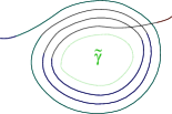
Figure 15: Parallel 2-encounter with internal triple revolution about periodic orbit $\tilde{\gamma}$

Figure 16: Overlap of parallel encounter stretches: a) An orbit $\gamma$ comes close to a shorter orbit $\tilde{\gamma}$ (dotted line); the “merged stretch” (full line) approaches $\tilde{\gamma}$ three times in the region ${\cal A}$ and twice in the region ${\cal B}$. b) An “isolated stretch” (dashed line) of $\gamma$ approaches ${\cal A}$ twice and ${\cal B}$ once. Also depicted is a Poincaré section ${\cal P}$ inside the region ${\cal B}$. c) The partner $\gamma^{\prime}$ has one repetition of $\tilde{\gamma}$ shifted between the merged stretch and the isolated stretch. d), e) Two shorter 3-encounters (depicted by thick lines) can be found in the region ${\cal A}$. They pierce three times through a Poincaré section ${\cal P}$ inside ${\cal A}$.

Sticking to the double-revolution case of Fig. 16a one might wonder why it is at all appropriate to speak of a 2-encounter, given the closeness of three substretches in part ${\cal A}$. One justification was in fact already mentioned: We may imagine the encounter in question generated by shrinking away one external loop from a standard 2-encounter. Another motivation is that of the three close substretches in part ${\cal A}$ ($n+1$ in the case of $n$ revolutions about $\tilde{\gamma}$) only two are independent; the third (the $n-1$ others) are uniquely determined by two, calculable through the linearized equations of motion.

Clearly, if one tries to reconnect (sub-)stretches of a parallel 2-encounter one does not get an acceptable partner orbit of $\gamma$ but a pseudo-orbit. However, the foregoing discussion carries over to parallel stretches in arbitrary $l$-encounters. For instance, by shrinking away an external loop from a parallel 3-encounter $\mathrel{\,\lower 0.6458pt\hbox{\begin{picture}(4.0,3.0)\put(0.0,0.3){\vector(1,0){4.0}}\put(0.0,1.5){\vector(1,0){4.0}} \put(0.0,2.7){\vector(1,0){4.0}} \end{picture}}\,}$ we arrive at Fig. 16b. Here the full line revolves twice about some $\tilde{\gamma}$ and thus is the “merger” of two “overlapping” parallel encounter stretches as in Fig. 16a, while the dashed line revolves only once around $\tilde{\gamma}$. The 3-encounter of $\gamma$ in question thus includes a “merged” stretch ${\cal A}{\cal B}{\cal A}{\cal B}{\cal A}$ and an “isolated” stretch ${\cal E}={\cal A}{\cal B}{\cal A}$.

Now a partner orbit $\gamma^{\prime}$ may arise wherein the dashed stretch has pinched one revolution about $\tilde{\gamma}$ from the full one (see Fig. 16c), a fact we now turn to explain. Recall that we can construct a partner orbit by changing connections inside the encounter. To do so, we place a Poincaré section within the encounter, say in region ${\cal B}$ as in Fig. 16b. The orbit $\gamma$ will pierce through that section in three points; the whole of $\gamma$, the external loops included, is thus divided into three parts. To determine the partner $\gamma^{\prime}$, we change the connections between these parts, and thus their ordering. The change of connections can be interpreted as cutting out one of the parts and reinserting it between the two other parts. In the case depicted in Fig. 16b, the merged stretch pierces through ${\cal P}$ twice, and the part of $\gamma$ between these piercings is one revolution about $\tilde{\gamma}$. The third piercing belongs to the isolated stretch. The partner $\gamma^{\prime}$ is thus obtained by cutting out one revolution about $\tilde{\gamma}$ from the merged stretches and inserting it inside the isolated one; see Fig. 16c. To translate to symbolic dynamics, we label the two remaining loops of $\gamma$ by ${\cal L}_{1}$ and ${\cal L}_{2}$ such that $\gamma={\cal L}_{1}({\cal A}{\cal B}{\cal A}{\cal B}{\cal A}){\cal L}_{2}({\cal A}{\cal B}{\cal A})$. The partner orbit $\gamma^{\prime}$ has one $\tilde{\gamma}={\cal A}{\cal B}$ shifted between the two stretches, i.e. $\gamma^{\prime}={\cal L}_{1}({\cal A}{\cal B}{\cal A}){\cal L}_{2}({\cal A}{\cal B}{\cal A}{\cal B}{\cal A})$.

It is important to note that the encounter shown in Fig. 16b may be represented by three pieces ${\cal A}$, two from the merged stretch and one from the isolated stretch. In other words, it suffices to consider a shorter encounter made of three independent traversals of the region ${\cal A}$. For example, we may take an encounter consisting of the first and second traversal of ${\cal A}$ by the merged stretch and the latest traversal by the isolated stretch; these traversals are depicted in Fig. 16d by thick full and dotted lines. We shall refer to the full 3-encounter and its shorter representative as to the “long” and “short” one.

The choice of the three representative traversals in the short encounter is not arbitrary. First, we have to make sure that the encounter is limited by the boundaries of ${\cal A}$. For the above example, we easily check that outside these boundaries, at least one of the traversing stretches starts to depart from the others. We have thus identified a shorter 3-encounter whose stretches do not overlap.

Second, we want our short encounter to give rise to the same partner orbit as the long one. To check this, let us place a Poincaré section somewhere inside ${\cal A}$; see Fig. 16d. Again, the two piercings of the merged stretch are separated by one revolution of $\tilde{\gamma}$, and there is one piercing by the isolated stretch. Just like for the larger encounter, the partner has one revolution of $\tilde{\gamma}$ cut out of the merged stretch and reinserted into the isolated one.

Both restrictions are fulfilled only for one further short 3-encounter, consisting of the second and third traversal by the merged stretch and the first traversal by the isolated stretch; see Fig. 16e.

For a first generalization we drop the above restriction on the length of the “overlapping part” within the merged stretch of a parallel 3-encounter. In general, all three encounter stretches must have the form ${\cal E}=({\cal A}{\cal B})^{n-1}{\cal A}$, $n\geq 2$, where the overlapping part is given by $({\cal A}{\cal B})^{n-2}{\cal A}$ (the above case referred to $n=2$). The merger of two of these reads $({\cal A}{\cal B})^{n}{\cal A}$ and executes $n$ revolutions about $\tilde{\gamma}={\cal A}{\cal B}$, whereas the isolated stretch remains as ${\cal E}=({\cal A}{\cal B})^{n-1}{\cal A}$ and revolves only $n-1$ times. Next, we would like to generalize to parallel $l$-encounters with larger $l$. If two of the stretches involved merge into one, this leaves $l-2$ isolated stretches with symbol sequences as above. As before, the partner orbit $\gamma^{\prime}$ has one revolution about $\tilde{\gamma}={\cal A}{\cal B}$ cut out of the merged stretch and inserted into one of the isolated stretches. In addition, the ordering of the intervening loops may be changed. Finally, given time-reversal invariance, the isolated stretches may also have symbol sequences time-reversed w.r.t. $({\cal A}{\cal B})^{n-1}{\cal A}$.

For all three generalizations just mentioned, we can identify a shorter encounter without overlap, consisting of $l$ traversals of the region ${\cal A}$, and that shorter representative suffices to get all partner orbits $\gamma^{\prime}$. To do so, we divide the stretches of the larger encounter in two groups. For each stretch of the first group, the earliest traversal of ${\cal A}$ will be included in the shorter encounter. For each stretch of the second group, we choose the latest traversal of ${\cal A}$. For the “merged” stretch also the second traversal of ${\cal A}$ needs to be included (or the next-to-last, if the merged stretch forms part of the second group). These $l$ traversals were chosen such that before the beginning of ${\cal A}$, the traversals of the first group deviate from the others, while the traversals of the second group do so after the end of ${\cal A}$. One further short encounter is built out of the latest traversals by the first group, and the earliest traversals by the second group. As before, we disregard the long encounter in favor of the shorter ones. Note that the division of stretches in two groups is not arbitrary; the groups must be chosen to guarantee that the shorter encounters give rise to the same partner as the larger one. (See MuellerPhD for details, and HeuslerPhD ; MuellerPhD for an alternative description of overlap in parallel 3-encounters.)

To sum up, each orbit pair generated by overlapping parallel stretches within some encounter can be thought of as originating from any of two shorter encounters without overlapping stretches. One of these two shorter encounters will, in the following subsection, be excluded and a one-to-one correspondence between orbit pairs and encounters will be reestablished, in effect by the condition (100) for the separation of piercings. As regards the form factor that condition will turn out semiclassically equivalent to the weaker condition (99), i.e. the requirement of non-vanishing loops we had worked with in the main part of this paper.

D.3 Fringes

Recall that we define an $l$-encounter as a region inside a periodic orbit in which $l$ orbit stretches come close up to time reversal. Attached to the sides of the encounter are “fringes” in which only some of the $l$ stretches remain close while others have already gone astray, as shown in Fig. 17a. We shall now show that these fringes do not affect the spectral form factor.

Figure 17: 3-encounter (in the box) with a “fringe” where only two antiparallel stretches remain close. Stretches are separated by a loop in a) but not in b); an almost self-retracing reflection arises in the latter case. A partner orbit (dashed line) is obtained only in case a).

As a first example, let us assume that two antiparallel stretches remain close after the end of the encounter, as in Fig. 17a. If there is no intervening loop (see Fig. 17b), the orbit has to undergo an almost self-retracing reflection, just like the one studied in Appendix D.1. Since no connections can be switched between the two stretches involved we have to disregard such encounters.

On the other hand, if the “fringe” stretches are separated by an external loop, a partner orbit is obtained as usual, by reshuffling connections inside the encounter, see Fig. 17a. To make sure that there is an intervening loop, we impose minimal separations between piercing points, similar to those used for excluding overlap between encounters in II.5. After two antiparallel stretches (labelled by $j$ and $j+1$) have pierced through a Poincaré section ${\cal P}$ with unstable coordinates $\hat{u}_{\alpha j}$ and $\hat{u}_{\alpha,j+1}$, they will remain close for a time $\frac{1}{\lambda}\ln\frac{c}{|\hat{u}_{\alpha j}-\hat{u}_{\alpha,j+1}|}$. This duration contains both the time $t_{u}$ (II.2) till the end of the $\alpha$-th encounter, and an additional time span after the end of the encounter, which gives the duration of the fringe. Using the unstable coordinates $\hat{u}_{\alpha j}^{\rm e}$ of piercing through a section in the end of the encounter (depending on $\hat{u}_{\alpha j}$ via $\hat{u}_{\alpha j}^{\rm e}=\hat{u}_{\alpha j}{\rm e}^{\lambda t_{u}}$), this additional time may be written as $\frac{1}{\lambda}\ln\frac{c}{|\hat{u}_{\alpha j}^{\rm e}-\hat{u}_{\alpha,j+1}^{\rm e}|}$.

Hence, the minimal time difference $2t_{u}$ between piercings demanded in II.5 has to be incremented by a time $t_{\rm fringe}=\frac{2}{\lambda}\ln\frac{c}{|\hat{u}_{\alpha j}^{\rm e}-\hat{u}_{\alpha,j+1}^{\rm e}|}$, depending on $\hat{u}$ (or, equivalently, the coordinates $u$ defined in II.3.2) only via $\hat{u}^{\rm e}$ (or, equivalently, $u^{\rm e}$). Similarly, the minimal separations related to stable coordinates have to be incremented by an amount purely depending on the stable coordinates $s^{\rm b}$ in the beginning of the encounter. The contribution of each encounter to the total sum of minimal separations $t_{\rm excl}$ can therefore be written in the form

$$t_{\rm excl}^{\alpha}=l_{\alpha}t_{\rm enc}^{\alpha}+\Delta t_{s}^{\alpha}(s^{{\rm b}})+\Delta t_{u}^{\alpha}(u^{{\rm e}})$$ (101)

with $\Delta t_{s}$ and $\Delta t_{u}$ respective functions of $s^{\rm b}$ and $u^{\rm e}$ only (whose explicit form will not be needed in the following). The numerator in the density of phase-space separations $w_{T}(s,u)$ (18) has to be modified accordingly.

By reasoning as in Subsection II.6, we see that only those terms of the multinomial expansion of the numerator in $w_{T}(s,u)$ contribute which involve a product of all $t_{\rm excl}^{\alpha}$. They now have to be written as (compare (II.6))

$$\frac{w_{T}^{\rm contr}(s,u)}{L} = h(\vec{v})\left(\frac{T}{\Omega}\right)^{L-V}\prod_{\alpha}\frac{t_{\rm excl}^{\alpha}}{l_{\alpha}t_{\rm enc}^{\alpha}}$$

$$= h(\vec{v})\left(\frac{T}{\Omega}\right)^{L-V}\prod_{\alpha}\left[1+\frac{\Delta t_{s}^{\alpha}+\Delta t_{u}^{\alpha}}{l_{\alpha}t_{\rm enc}^{\alpha}}\right],$$

and contribute to the form factor as (compare (24))

$$\kappa\tau h(\vec{v})\left(\frac{T}{\Omega}\right)^{L-V}\prod_{\alpha}\left[\int d^{L-V}s\;d^{L-V}u\right.$$

$$\left.\left(1+\frac{\Delta t_{s}^{\alpha}(s^{{\rm b}})+\Delta t_{u}^{\alpha}(u^{{\rm e}})}{l_{\alpha}t_{\rm enc}^{\alpha}}\right){\rm e}^{\frac{\rm i}{\hbar}\sum_{j}s_{\alpha j}u_{\alpha j}}\right]\,.$$ (102)

The integral in (D.3) coincides with the one in (24) up to the fringe corrections $\propto\frac{\Delta t_{s}^{\alpha}}{t_{\rm enc}^{\alpha}}$ and $\propto\frac{\Delta t_{u}^{\alpha}}{t_{\rm enc}^{\alpha}}$, respectively. By reasoning similar to Appendix A, one easily shows that the resulting integrals vanish in the semiclassical limit. For the integrand $\frac{\Delta t_{u}^{\alpha}}{t_{\rm enc}^{\alpha}}$, the rapidly oscillating integral over $s_{J}^{\rm e}$ inside (91) is not modified; for $\frac{\Delta t_{s}^{\alpha}}{t_{\rm enc}^{\alpha}}$ we have to consider a surface of section in the beginning rather than in the end of the encounter. For antiparallel orbit stretches, fringe corrections to the form factor are hence revealed as negligible semiclassically.

Let us now consider fringes of parallel encounter stretches. In the absence of intervening loops, there may be different encounters yielding the same partner orbit, like the two short encounters of Appendix D.2, depicted in Fig. 16d and e. One easily sees that these short encounters do not have their fringes separated by loops. For instance, in Fig. 16d, the two full thick stretches remain close after the end of the encounter region ${\cal A}$, thus forming a fringe. They are still close when the orbit reenters ${\cal A}$, such that there is no external loop.

In order to count the resulting partner $\gamma^{\prime}$ exactly once, we choose to take into account only the encounter in Fig. 16e, and disregard the one in Fig. 16d. To do so, we again have to increase the minimal distances between piercing points; see (100). As above, the increment $t_{\rm fringe}$ may depend only on $s^{\rm b}$ and $u^{\rm e}$, given that these quantities determine how long each two stretches will stay close inside the fringe region. More precisely, one can even show that $t_{\rm fringe}$ is given by a sum of two terms depending on $s^{\rm b}$ and $u^{\rm e}$, respectively. (For instance, for the first two piercings of a 3-encounter, $t_{\rm fringe}=\frac{1}{\lambda}\ln\frac{c}{|\hat{u}_{\alpha 1}^{\rm e}-\hat{u}_{\alpha 2}^{\rm e}|}+\frac{1}{\lambda}\ln\frac{c}{|\hat{s}_{\alpha 2}^{\rm b}-\hat{s}_{\alpha 3}^{\rm b}|}$; see MuellerPhD for the derivation and a generalization to arbitrary $l$-encounters.) Hence, the sum of all minimal distances will still be of the form (101); the increment will thus not contribute to $K(\tau)$ in the semiclassical limit.

The present treatment immediately generalizes to $f>2$, by writing out the additional index $k$, and to non-homogeneously hyperbolic systems by keeping the dependence on ${\bf x}$. In particular, $\Delta t_{s}$ will depend both on $s^{\rm b}$ and the phase-space points ${\bf x}^{\rm b}$ in the beginning of the encounter, and $\Delta t_{u}$ on $u^{\rm e}$ and ${\bf x}^{\rm e}$ in the end of the encounter.

Appendix E The nonlinear $\sigma$-model

E.1 Replica trick and perturbation expansion

We here sketch the derivation of the integral representation (79) for the Wigner/Dyson ensembles. For simplicity, we concentrate on the GUE. For the GOE see Subsection E.2 below. We start from the “replica representation” of the Green function $G(z)\equiv(z-H)^{-1}$,

$${\rm tr}\,G(z) = \partial_{z}{\,\rm tr}\ln(G(z)^{-1})=\partial_{z}\ln({\rm det\,}G(z)^{-1})$$ (103)

$$= -\lim_{r\to 0}{1\over r}\partial_{z}\det G(z)^{r}\,.$$

We take the Hamiltonian $H$ as an $N$-dimensional Hermitian random matrix whose Gaussian statistics is defined by the two moments

$$\overline{H_{\mu\nu}}=0,$$

$$\overline{H_{\mu\nu}\,H_{\nu^{\prime}\mu^{\prime}}}=\frac{\lambda^{2}}{N}\delta_{\mu\mu^{\prime}}\delta_{\nu\nu^{\prime}}\,;$$ (104)

these imply Wigner’s semicircle for the mean level density as $\overline{\rho}(E)=(N/\pi\lambda^{2})\sqrt{\lambda^{2}-(E/2)^{2}}\,\Theta(\lambda^{2}-(E/2)^{2})$ and thus the mean spacing $\pi\lambda/N$ at $E=0$.

The $r$th power of the determinant in (103) can be written as the Gaussian integral (summation convention)

$$\det(G(z))^{r}=\int d\psi\,\exp(\pm{\rm i}\psi^{a\dagger}(z-H)\psi^{a})\,;$$ (105)

here $\psi^{a}=\{\psi^{a}_{\mu}\}$, $a=1,\ldots,r$ are $N$–dimensional complex vectors of integration variables; the measure $d\psi\propto\prod_{\mu=1}^{N}\prod_{a=1}^{r}d{\rm Re}\psi_{\mu}^{a}d{\rm Im}\psi_{\mu}^{a}$ comprises a normalization constant of the form $({\rm const})^{r}\sim 1$; here and in the remainder of this Appendix we let the symbol $\sim$ mean equality in the limit $r\to 0$; the positive/negative sign in the exponent applies to the case ${\rm Im\,}z>0$/${\rm Im\,}z<0$.

We proceed to the retarded and advanced Green functions ${\rm tr}\,G_{\pm}(E)={\rm tr}\,G(E\pm{\rm i}\delta)$ with real $E$ and $\delta\downarrow 0$. Their ensemble averaged product

$$C(\epsilon)=\overline{{(\rm tr}\,G_{+}(E+\epsilon/2))({\rm tr}\,G_{-}(E-\epsilon/2))}$$ (106)

leads to the spectral correlator and the form factor according to (V.2). Applying the replica trick (103) and the integral representation (105) twice, i.e. both for $G_{+}$ and $G_{-}$, we get to a bosonic replica variant of the sigma model: the correlation function $C(\epsilon)$ appears as a two–fold derivative of a generating function,

$$C(\epsilon) = \lim_{r\to 0}\frac{1}{r^{2}}\left[\frac{\partial^{2}Z(\hat{\epsilon})}{\partial\epsilon_{+}\partial\epsilon_{-}}\right]_{\epsilon_{\pm=\pm\frac{\epsilon}{2}}}\,,$$ (107)

$$\mathcal{Z}(\hat{\epsilon}) = \int d\psi\,\overline{\exp({\rm i}\psi^{\dagger}\Lambda(\hat{\epsilon}+E-H)\psi)}\,,$$ (108)

$$\hat{\epsilon} = \mathrm{\,diag\,}(\epsilon_{+}+{\rm i}\delta,\epsilon_{-}-{\rm i}\delta)\,,\quad\delta\downarrow 0\,,$$

$$\Lambda = \mathrm{\,diag\,}(1,-1)\,.$$

Compared to (105) the number of integrations is doubled in the generating function $\mathcal{Z}$: a doublet $\psi\equiv(\psi^{1},\psi^{2})$ comprises $rN$–dimensional vectors $\psi^{1}$ and $\psi^{2}$ needed to represent the retarded and the advanced Green functions by Gaussian integrals. The diagonal matrices $\hat{\epsilon},\Lambda$ act in the newly introduced advanced/retarded space like $\Lambda{\psi^{1}\choose\psi^{2}}={\psi^{1}\choose-\psi^{2}}$, and like unity in the replica space. Note that $\Lambda$ and the imaginary part of $\hat{\epsilon}$ together secure convergence of the Gaussian integrals in $\mathcal{Z}$ as did the plus/minus sign in (105). The replica index $a$ is suppressed in the compact notation for $\mathcal{Z}$.

The GUE average is now easily done in (108) since the random Hamiltonian appears linearly in the exponent,

$$\mathcal{Z}(\hat{\epsilon})=\!\int\!d\psi\,\exp\!\left(\!{\rm i}\psi^{\dagger}\Lambda(\hat{\epsilon}+E)\psi-\frac{\lambda^{2}}{2N}{\rm tr\,}A^{2}\!\right)$$

with the $2r\times 2r$ matrix $A=\{A^{\alpha\beta}=\sum_{\mu=1}^{N}\psi_{\mu}^{\alpha}\psi_{\mu}^{\beta\ast}\Lambda^{\beta\beta}\}$; the index $\alpha=(p,a)$ comprises the replica index $a=1\ldots r$ and an index $p=1,2$ discriminating between “advanced” and “retarded”. We next decouple the term $\propto{\rm tr}\,A^{2}$ quartic in the integration variables $\psi$ by a Hubbard–Stratonovich transformation. To this end, we multiply $\mathcal{Z}$ by the unit–normalized Gaussian integral $1=\mathcal{N}\int dQ\,\exp\left(\frac{N}{2}{\rm tr}\,Q^{2}\right)$, where $Q=\{Q^{\alpha\beta}\}$ is a $2r$–dimensional anti-Hermitian matrix and $\int dQ$ denotes integration over all its independent matrix elements; the latter comprise $(2r)^{2}$ independent real and imaginary parts such that the normalization constant is of the form ${\mathcal{N}}=({\rm const})^{r^{2}}\sim 1$. The shift $Q\to Q-\lambda A/N$ leads to

$$\mathcal{Z}(\hat{\epsilon})\!\! \sim \!\!\!\!\!\int\!\!d\psi\!\int\!\!dQ\exp\!\left({\textstyle{\frac{N}{2}}}{\rm tr}\,Q^{2}+{\rm i}\psi^{\dagger}\Lambda(\hat{\epsilon}+E+{\rm i}\lambda Q)\psi\right)$$

$$\sim \!\!\!\!\int\!\!dQ\,\exp\left({\textstyle{\frac{N}{2}}}{\rm tr}\,Q^{2}-N{\rm\,tr\,ln}(\hat{\epsilon}+E+{\rm i}\lambda Q)\right)\;\;\;\;\;\;$$

where in the second step we have performed the Gaussian integration over $\psi$. The large parameter $N$ in the foregoing exponential allows for a stationary-phase approximation of the $Q$–integral. Variation of the exponent, the so-called action, w.r.t. the independent matrix elements of $Q$ yields the saddle-point equation

$$Q=\frac{{\rm i}\lambda}{\hat{\epsilon}+E+{\rm i}\lambda Q}\,.$$ (109)

In order to shorten the saddle-point analysis we confine ourselves to $E=0$; the final result is valid throughout Wigner’s semicircle. The saddle-point equation then invites solution to zeroth order in $\hat{\epsilon}$ since the scale for the energy offset variables is the mean level spacing, $\epsilon_{\pm}=\mathcal{O}(N^{-1})$; we can even dispatch the infinitesimal imaginary part $\mathrm{Im}(\hat{\epsilon})={\rm i}\Lambda\delta$ which is only needed to ensure absolute convergence of all integrals. A simple matrix–diagonal saddle point thus arises, $Q\simeq\Lambda$. (Strictly speaking, there are $2^{2r}$ diagonal solutions with diagonal entries $\pm 1$. However, the solutions different from $\Lambda=\mathrm{\,diag\,}(1,-1)$, have to be discarded since they cannot be reached without crossing the cuts of the logarithm in the action Weidenmueller ).

A continuous manifold of more general (non–diagonal yet compatible with the cut structure of the logarithm) solutions of the saddle-point equation can now be obtained by the conjugation $\Lambda\to T\Lambda T^{-1}\equiv Q_{\rm s}$, where $T\in{\rm U}(r,r)$ is a $(2r)$–dimensional pseudo-unitary matrix. (The pseudounitarity condition, $T\Lambda T^{\dagger}=\Lambda$, is required to make the subsequent integration over all configurations $Q$ convergent SymmSpaces .) This observation identifies the non–compact symmetric space ${\rm U}(r,r)/{\rm U}(r)\times{\rm U}(r)$ as the saddle-point manifold. (Transformations $T\in{\rm U}(r)\times{\rm U}(r)$ commute with $\Lambda$ and, therefore, do not affect the diagonal saddle.) It may be a noteworthy property of the saddle-point manifold in question that the matrices $Q$ thereon are no longer anti-Hermitian SymmSpaces .

We next substitute the saddle configurations $Q_{\rm s}=T\Lambda T^{-1}$ into the action and expand to order $\hat{\epsilon}$,

$$\mathcal{Z}(\hat{\epsilon}) \sim \int dQ_{\rm s}\,\exp\left(-N{\rm\,tr\,}\left[\hat{\epsilon}(E+{\rm i}\lambda Q_{\rm s})^{-1}\right]\right)$$ (110)

$$\stackrel{{\scriptstyle(\ref{eq:pastur_eq})}}{{\sim}} \int dQ_{\rm s}\,\exp\left({{\rm i}N\over\lambda}{\rm\,tr\,}\left[\hat{\epsilon}Q_{\rm s}\right]\right)$$

$$\sim \int dQ_{\rm s}\,\exp\left({{\rm i}(\epsilon_{+}-\epsilon_{-}+{\rm i}2\delta)\pi\bar{\rho}\over 2}{\rm\,tr\,}\left[\Lambda Q_{\rm s}\right]\right)$$

$$\sim \int dQ_{\rm s}\,\exp{\left(\frac{{\rm i}s^{+}}{2}{\rm tr}\Lambda Q_{\rm s}\right)}\,,$$

where now $\int dQ_{\rm s}$ demands integration over the saddle-point manifold Weidenmueller ; in the foregoing calculation we used that ${\rm tr}(Q_{\rm s}^{2})={\rm tr}(\Lambda^{2})=r\sim 0$ and that ${\rm tr}(Q_{\rm s}\hat{\epsilon})=(\epsilon_{+}+\epsilon_{-}){\rm tr}(Q_{\rm s})/2+(\epsilon_{+}-\epsilon_{-}+2{\rm i}\delta){\rm tr}(Q_{\rm s}\Lambda)/2=(\epsilon_{+}-\epsilon_{-}+2{\rm i}\delta){\rm tr}(Q_{\rm s}\Lambda)/2$; finally, in the last step we introduced the scaled offset $s^{+}=(\epsilon_{+}-\epsilon_{-}+2{\rm i}\delta)\pi\bar{\rho}$. In order to evaluate the matrix integral above we need an explicit parametrization of the $Q$–matrices on the saddle-point manifold. Taylor made to perturbative calculations is the so-called rational parametrization

$$Q_{\rm s}=(1-W)\Lambda(1-W)^{-1}\,;\;W=\frac{1}{\sqrt{s^{+}}}\left({0\atop B^{\dagger}}{B\atop 0}\right)$$ (111)

where the scaling factor $1/\sqrt{s^{+}}$ makes for notational convenience. The main merit of that representation is that the invariant measure $dQ_{\rm s}$ is effectively (i.e. in view of the eventual limit $r\to 0$) the flat measure $(s^{+})^{-r^{2}}\prod_{i,j}^{1\ldots r}d{\rm Re}B_{ij}d{\rm Im}B_{ij}\equiv(s^{+})^{-r^{2}}dB$ for $r\times r$ matrices $B$. Inserting the parametrization (111) in the generating function (110) we expand as $(1-W)^{-1}=\sum_{n=0}^{\infty}W^{n}$ to get

$$\mathcal{Z}(\hat{\epsilon})\sim(s^{+})^{-r^{2}}\,{\rm e}^{{\rm i}s^{+}r}\int{dB}\,{\rm e}^{(2{{\rm i}}/\kappa)\sum_{l=1}^{\infty}(s^{+})^{1-l}{\rm tr}(B{B^{\dagger}})^{l}}\,,$$ (112)

where the factor $\kappa=1$ has been sneaked in for later use.

We had shown in V.2 that the foregoing $B$-integral yields $\{{\rm const}^{r^{2}}+r^{2}f_{2}(s^{+})+r^{3}f_{3}(s^{+})+{\mathcal{O}}(r^{4})\}$ with $f_{i}(s^{+})$ polynomials in $1/s^{+}$. Therefore, nonzero contributions to the correlator $C(\epsilon)$ according to (107) arise only when both derivatives $\partial^{2}/\partial\epsilon_{+}\partial\epsilon_{-}$ act together on each of the three factors on the r. h. s. of (112). It is easy to see that the contribution from $\partial^{2}{\rm e}^{{\rm i}s^{+}r}/\partial\epsilon_{+}\partial\epsilon_{-}$ yields the disconnected part $\bar{\rho}^{2}$ such that upon simply setting ${\rm e}^{{\rm i}s^{+}r}\to 1$ and invoking (107) we get (the non-oscillatory contributions to) the connected part $C_{\rm conn}(\epsilon)$ instead of $C(\epsilon)$. The connected correlation function defined in (V.2) is thus obtained as $R=\frac{1}{2\pi^{2}\overline{\rho}^{2}}\mbox{Re}\,C_{\rm conn}=-\frac{1}{2}\mbox{Re}\frac{\partial^{2}}{\partial{s^{+}}^{2}}\big{(}Z|_{{\rm e}^{{\rm i}s^{+}r}\to 1}\big{)}$ which leads us to (79) for the unitary class, with $\kappa=1$.

E.2 Generalization to the orthogonal class

For the GOE, Eq. (104) generalizes to

$$\langle H_{\mu\nu}\rangle=0,$$

$$\langle H_{\mu\nu}\,H_{\nu^{\prime}\mu^{\prime}}\rangle=\frac{\lambda^{2}}{N}(\delta_{\mu\mu^{\prime}}\delta_{\nu\nu^{\prime}}+\delta_{\mu\nu^{\prime}}\delta_{\nu\mu^{\prime}})\,.$$

As a consequence, the averaged action will contain the sum of two contributions quartic in the integration variables, $\psi^{\dagger}_{\mu}\Lambda\psi_{\nu}\left(\psi^{\dagger}_{\nu}\Lambda\psi_{\mu}+\psi^{\dagger}_{\mu}\Lambda\psi_{\nu}\right)=2\bar{\Psi}_{\mu}\Lambda\Psi_{\nu}\bar{\Psi}_{\nu}\Lambda\Psi_{\nu}$, where we have defined

$$\bar{\Psi}\equiv\frac{1}{\sqrt{2}}(\psi^{\dagger},\psi^{T}),\qquad\Psi=\frac{1}{\sqrt{2}}\left(\begin{array}[]{c}\psi\cr\psi^{\ast}\end{array}\right).$$ (113)

Notice that the $4r$–component vectors $\Psi$ and $\bar{\Psi}$ are connected by the symmetry relation

$$\bar{\Psi}=\Psi^{T}\sigma_{1},$$ (114)

where the Pauli matrix $\sigma_{1}$ acts in the two–component space of Eq. (113). To decouple the quartic $\Psi$–term in the action, we introduce a $Q$–matrix subject to the constraint $Q=\sigma_{1}Q^{T}\sigma_{1}$. Noting that $\psi^{\dagger}(\hat{\epsilon}+E)\psi=\bar{\Psi}(\hat{\epsilon}+E)\Psi$ and proceeding as in the unitary case we get

$$\mathcal{Z}(\hat{\epsilon}) = \!\!\int\!\!d\Psi\!\!\int\!\!dQ\exp\!\left(\!{\textstyle{\frac{N^{2}}{4}}}{\rm tr}(Q^{2})+{\rm i}\bar{\Psi}\Lambda(\hat{\epsilon}+E+{\rm i}\lambda Q)\Psi\!\right)$$

$$= \!\!\int\!\!dQ\,\exp\left({\textstyle{\frac{N^{2}}{4}}}{\rm tr}(Q^{2})-{\textstyle{{N\over 2}}}{\rm\,tr\,ln}(\hat{\epsilon}+E+{\rm i}\lambda Q)\right),$$

where we made use of the symmetry of $Q$. A stationary-phase approach yields the diagonal saddle $Q=\Lambda$ and its non-diagonal generalization $Q_{\rm s}=T\Lambda T^{-1}$, where $T\in{\rm O}(2r,2r)$. (Compatibility with the symmetries of $Q$ requires $T^{T}=\sigma_{1}T^{-1}\sigma_{1}$, hence the restriction to the (pseudo)orthogonal group.) This identifies $\mathrm{O}(2r,2r)/\mathrm{O}(2r)\times\mathrm{O}(2r)$ as the saddle-point manifold.

As in the unitary case, we represent the $Q_{\rm s}$–matrices in the rational parametrization (111). Presently, time–reversal invariance implies $T^{T}=\sigma_{1}T^{-1}\sigma_{1}$ and, as the symmetry of the integration variables $B$,

$$B^{\dagger}=-\sigma_{1}B^{T}\sigma_{1}\,.$$ (115)

Simplifying the action to leading order in $\hat{\epsilon}$ and expanding in $W$, we recover Eq. (79), now with $\kappa=2$.

E.3 Contraction rules

To compute the matrix integral perturbatively in an expansion in $1/s^{+}$, one expands the exponentiated action in powers of traces ${\rm tr}[(BB^{\dagger})^{l}]$, $l~{}\!\!\!\!\geq~{}\!\!\!\!2$. This leads to a series of terms of the structure $\langle({\rm tr}[(BB^{\dagger})^{2}])^{v_{2}}({\rm tr}[(BB^{\dagger})^{3}])^{v_{3}}\dots\rangle$, where $v_{l}$ are integers and the averaging over the quadratic action, $\langle\dots\rangle$, is defined by (81). Each term contributing to the series is then computed by Wick’s theorem, i.e. as a sum over all non–vanishing pair contractions (85a-d) of $B$–matrices. We now briefly outline the derivation of the basic contraction rules. In an index notation, the quadratic action reads $S^{(2)}[B,B^{\dagger}]={({\rm i}/\kappa)}\sum_{\alpha\alpha^{\prime}}|B_{\alpha\alpha^{\prime}}|^{2}$. This implies the prototypical contraction rule

$$\langle B_{\alpha\alpha^{\prime}}{B^{\dagger}}_{\beta^{\prime}\beta}\rangle=-{1\over 2{\rm i}}\delta_{\alpha\beta}\delta_{\alpha^{\prime}\beta^{\prime}}\,,$$

the $\kappa$–independence of which follows from the fact that in the orthogonal case, $\kappa=2$, only one half of the matrix elements $B_{\alpha\alpha^{\prime}}$ are independent integration variables — a consequence of the time reversal relation (115). When expressed as a sum over independent integration variables only, the coefficient of the action effectively doubles, i.e. in either case $\kappa=1,2$ the integration over matrix components obtains a factor ${\rm i}/2$. Using this relation we obtain

$$\big{<}{\rm tr}\mathchoice{\vbox{\hbox to0.0pt{\kern 0.0pt\kern 3.54167pt\hbox{\vrule width=0.59998pt,height=0.0pt,depth=8.61108pt\vrule width=26.7083pt,height=0.0pt,depth=0.59998pt\vrule width=0.59998pt,height=0.0pt,depth=8.61108pt}\hss}\vskip 0.86108pt\vskip 6.83331pt}}{\vbox{\hbox to0.0pt{\kern 0.0pt\kern 3.54167pt\hbox{\vrule width=0.59998pt,height=0.0pt,depth=8.61108pt\vrule width=26.7083pt,height=0.0pt,depth=0.59998pt\vrule width=0.59998pt,height=0.0pt,depth=8.61108pt}\hss}\vskip 0.86108pt\vskip 6.83331pt}}{\vbox{\hbox to0.0pt{\kern 0.0pt\kern 2.47917pt\hbox{\vrule width=0.59998pt,height=0.0pt,depth=8.61108pt\vrule width=19.52911pt,height=0.0pt,depth=0.59998pt\vrule width=0.59998pt,height=0.0pt,depth=8.61108pt}\hss}\vskip 0.86108pt\vskip 4.78333pt}}{\vbox{\hbox to0.0pt{\kern 0.0pt\kern 1.77083pt\hbox{\vrule width=0.59998pt,height=0.0pt,depth=8.61108pt\vrule width=14.74298pt,height=0.0pt,depth=0.59998pt\vrule width=0.59998pt,height=0.0pt,depth=8.61108pt}\hss}\vskip 0.86108pt\vskip 3.41666pt}}{B}X\ {\rm tr}{{B^{\dagger}}}Y\big{>} = \big{<}\mathchoice{\vbox{\hbox to0.0pt{\kern 0.0pt\kern 3.54167pt\hbox{\vrule width=0.59998pt,height=0.0pt,depth=8.61108pt\vrule width=32.7751pt,height=0.0pt,depth=0.59998pt\vrule width=0.59998pt,height=0.0pt,depth=8.61108pt}\hss}\vskip 0.86108pt\vskip 6.83331pt}}{\vbox{\hbox to0.0pt{\kern 0.0pt\kern 3.54167pt\hbox{\vrule width=0.59998pt,height=0.0pt,depth=8.61108pt\vrule width=32.7751pt,height=0.0pt,depth=0.59998pt\vrule width=0.59998pt,height=0.0pt,depth=8.61108pt}\hss}\vskip 0.86108pt\vskip 6.83331pt}}{\vbox{\hbox to0.0pt{\kern 0.0pt\kern 2.47917pt\hbox{\vrule width=0.59998pt,height=0.0pt,depth=8.61108pt\vrule width=23.86253pt,height=0.0pt,depth=0.59998pt\vrule width=0.59998pt,height=0.0pt,depth=8.61108pt}\hss}\vskip 0.86108pt\vskip 4.78333pt}}{\vbox{\hbox to0.0pt{\kern 0.0pt\kern 1.77083pt\hbox{\vrule width=0.59998pt,height=0.0pt,depth=8.61108pt\vrule width=19.0764pt,height=0.0pt,depth=0.59998pt\vrule width=0.59998pt,height=0.0pt,depth=8.61108pt}\hss}\vskip 0.86108pt\vskip 3.41666pt}}{B_{\alpha\beta}}X_{\beta\alpha}{{B^{\dagger}_{\gamma\delta}}}Y_{\delta\gamma}\big{>}$$

$$= -{1\over 2{\rm i}}\langle X_{\beta\alpha}Y_{\alpha\beta}\rangle$$

$$= -{1\over 2{\rm i}}\langle{\rm tr}(X\,Y)\rangle,$$

which is contraction rule (85a). Rule (85b) is proven in the same manner. Rule (85d) for the GOE results from

$$\langle{\rm tr}\mathchoice{\vbox{\hbox to0.0pt{\kern 0.0pt\kern 4.0434pt\hbox{\vrule width=0.59998pt,height=0.0pt,depth=8.61108pt\vrule width=16.51042pt,height=0.0pt,depth=0.59998pt\vrule width=0.59998pt,height=0.0pt,depth=8.61108pt}\hss}\vskip 0.86108pt\vskip 6.83331pt}}{\vbox{\hbox to0.0pt{\kern 0.0pt\kern 4.0434pt\hbox{\vrule width=0.59998pt,height=0.0pt,depth=8.61108pt\vrule width=16.51042pt,height=0.0pt,depth=0.59998pt\vrule width=0.59998pt,height=0.0pt,depth=8.61108pt}\hss}\vskip 0.86108pt\vskip 6.83331pt}}{\vbox{\hbox to0.0pt{\kern 0.0pt\kern 2.83037pt\hbox{\vrule width=0.59998pt,height=0.0pt,depth=8.61108pt\vrule width=11.55728pt,height=0.0pt,depth=0.59998pt\vrule width=0.59998pt,height=0.0pt,depth=8.61108pt}\hss}\vskip 0.86108pt\vskip 4.78333pt}}{\vbox{\hbox to0.0pt{\kern 0.0pt\kern 2.0217pt\hbox{\vrule width=0.59998pt,height=0.0pt,depth=8.61108pt\vrule width=8.25519pt,height=0.0pt,depth=0.59998pt\vrule width=0.59998pt,height=0.0pt,depth=8.61108pt}\hss}\vskip 0.86108pt\vskip 3.41666pt}}{B}X{{B}}Y\rangle = \langle{\rm tr}((\sigma_{1}X)\mathchoice{\vbox{\hbox to0.0pt{\kern 0.0pt\kern 4.0434pt\hbox{\vrule width=0.59998pt,height=0.0pt,depth=8.61108pt\vrule width=46.80766pt,height=0.0pt,depth=0.59998pt\vrule width=0.59998pt,height=0.0pt,depth=8.61108pt}\hss}\vskip 0.86108pt\vskip 6.83331pt}}{\vbox{\hbox to0.0pt{\kern 0.0pt\kern 4.0434pt\hbox{\vrule width=0.59998pt,height=0.0pt,depth=8.61108pt\vrule width=46.80766pt,height=0.0pt,depth=0.59998pt\vrule width=0.59998pt,height=0.0pt,depth=8.61108pt}\hss}\vskip 0.86108pt\vskip 6.83331pt}}{\vbox{\hbox to0.0pt{\kern 0.0pt\kern 2.83037pt\hbox{\vrule width=0.59998pt,height=0.0pt,depth=8.61108pt\vrule width=34.34532pt,height=0.0pt,depth=0.59998pt\vrule width=0.59998pt,height=0.0pt,depth=8.61108pt}\hss}\vskip 0.86108pt\vskip 4.78333pt}}{\vbox{\hbox to0.0pt{\kern 0.0pt\kern 2.0217pt\hbox{\vrule width=0.59998pt,height=0.0pt,depth=8.61108pt\vrule width=27.10373pt,height=0.0pt,depth=0.59998pt\vrule width=0.59998pt,height=0.0pt,depth=8.61108pt}\hss}\vskip 0.86108pt\vskip 3.41666pt}}{B}(Y\sigma_{1})\,(\sigma_{1}{{B}}\sigma_{1}))\rangle$$

$$= \langle(\sigma_{1}X)_{\alpha\beta}\mathchoice{\vbox{\hbox to0.0pt{\kern 0.0pt\kern 3.54167pt\hbox{\vrule width=0.59998pt,height=0.0pt,depth=8.61108pt\vrule width=58.08316pt,height=0.0pt,depth=0.59998pt\vrule width=0.59998pt,height=0.0pt,depth=8.61108pt}\hss}\vskip 0.86108pt\vskip 6.83331pt}}{\vbox{\hbox to0.0pt{\kern 0.0pt\kern 3.54167pt\hbox{\vrule width=0.59998pt,height=0.0pt,depth=8.61108pt\vrule width=58.08316pt,height=0.0pt,depth=0.59998pt\vrule width=0.59998pt,height=0.0pt,depth=8.61108pt}\hss}\vskip 0.86108pt\vskip 6.83331pt}}{\vbox{\hbox to0.0pt{\kern 0.0pt\kern 2.47917pt\hbox{\vrule width=0.59998pt,height=0.0pt,depth=8.61108pt\vrule width=41.1485pt,height=0.0pt,depth=0.59998pt\vrule width=0.59998pt,height=0.0pt,depth=8.61108pt}\hss}\vskip 0.86108pt\vskip 4.78333pt}}{\vbox{\hbox to0.0pt{\kern 0.0pt\kern 1.77083pt\hbox{\vrule width=0.59998pt,height=0.0pt,depth=8.61108pt\vrule width=31.95166pt,height=0.0pt,depth=0.59998pt\vrule width=0.59998pt,height=0.0pt,depth=8.61108pt}\hss}\vskip 0.86108pt\vskip 3.41666pt}}{B_{\beta\gamma}}(Y\sigma_{1})_{\gamma\delta}(\sigma_{1}{{B}}\sigma_{1})_{\delta\alpha}\rangle$$

$$\stackrel{{\scriptstyle~{}(\ref{sigma_time_reversal})}}{{=}} -\langle(\sigma_{1}X)_{\alpha\beta}\mathchoice{\vbox{\hbox to0.0pt{\kern 0.0pt\kern 3.54167pt\hbox{\vrule width=0.59998pt,height=0.0pt,depth=8.61108pt\vrule width=45.9579pt,height=0.0pt,depth=0.59998pt\vrule width=0.59998pt,height=0.0pt,depth=8.61108pt}\hss}\vskip 0.86108pt\vskip 6.83331pt}}{\vbox{\hbox to0.0pt{\kern 0.0pt\kern 3.54167pt\hbox{\vrule width=0.59998pt,height=0.0pt,depth=8.61108pt\vrule width=45.9579pt,height=0.0pt,depth=0.59998pt\vrule width=0.59998pt,height=0.0pt,depth=8.61108pt}\hss}\vskip 0.86108pt\vskip 6.83331pt}}{\vbox{\hbox to0.0pt{\kern 0.0pt\kern 2.47917pt\hbox{\vrule width=0.59998pt,height=0.0pt,depth=8.61108pt\vrule width=32.70415pt,height=0.0pt,depth=0.59998pt\vrule width=0.59998pt,height=0.0pt,depth=8.61108pt}\hss}\vskip 0.86108pt\vskip 4.78333pt}}{\vbox{\hbox to0.0pt{\kern 0.0pt\kern 1.77083pt\hbox{\vrule width=0.59998pt,height=0.0pt,depth=8.61108pt\vrule width=25.42793pt,height=0.0pt,depth=0.59998pt\vrule width=0.59998pt,height=0.0pt,depth=8.61108pt}\hss}\vskip 0.86108pt\vskip 3.41666pt}}{B_{\beta\gamma}}(Y\sigma_{1})_{\gamma\delta}{{B^{\dagger}_{\alpha\delta}}}\big{>}$$

$$= +{1\over 2{\rm i}}\langle(\sigma_{1}X)_{\alpha\beta}(\sigma_{1}Y^{T})_{\beta\alpha}\rangle$$

$$= +{1\over 2{\rm i}}\langle{\rm tr}(X(\sigma_{1}Y^{T}\sigma_{1}))\rangle$$

$$= -{1\over 2{\rm i}}\langle{\rm tr}(X\,Y^{\dagger})\rangle\,,$$

where in the last step we used that $Y$ contains an odd number of matrices $B$ and $B^{\dagger}$ (i.e. that the time reversal relation (115) implies $\sigma_{1}Y^{T}\sigma_{1}=-Y^{\dagger}$.) The proof of rule (85c) proceeds along the same lines.

References

- (1) O. Bohigas, M. J. Giannoni, and C. Schmit, Phys. Rev. Lett. 52, 1 (1984); G. Casati, F. Valz-Gris, and I. Guarneri, Lett. Nuovo Cim. 28, 279 (1980); M. V. Berry, Ann. Phys. (N.Y.) 131, 163 (1981).
- (2) H.-J. Stöckmann, Quantum Chaos: An Introduction (Cambridge University Press, Cambridge, England, 1999).
- (3) F. Haake, Quantum Signatures of Chaos (Springer, Berlin, 2nd ed 2001).
- (4) M. L. Mehta, Random Matrices and the Statistical Theory of Spectra (Academic, New York, 2nd ed 1991).
- (5) M. V. Berry, Proc. R. Soc. Lond., Ser. A 400, 229 (1985).
- (6) N. Argaman, F.-M. Dittes, E. Doron, J. P. Keating, A. Yu. Kitaev, M. Sieber, and U. Smilansky, Phys. Rev. Lett. 71, 4326 (1993).
- (7) M. Sieber and K. Richter, Physica Scripta T90, 128 (2001); M. Sieber, J. Phys. A 35, L613 (2002).
- (8) M. Gutzwiller, Chaos in Classical and Quantum Mechanics (Springer, New York, 1990).
- (9) D. Cohen, H. Primack, and U. Smilansky, Ann. Phys. 264, 108 (1998).
- (10) H. Primack and U. Smilansky, Phys. Rep. 327, 1 (2000).
- (11) U. Smilansky and B. Verdene, J. Phys. A 36, 3525 (2003).
- (12) I. L. Aleiner and A. I. Larkin, Phys. Rev. B 54, 14423 (1996).
- (13) R. A. Smith, I. V. Lerner, and B. L. Altshuler, Phys. Rev. B 58, 10343 (1998); R. S. Whitney, I. V. Lerner, and R. A. Smith, Waves Random Media 9, 179 (1999).
- (14) S. Müller, Eur. Phys. J. B 34, 305 (2003); Diplomarbeit, Universität Essen (2001).
- (15) D. Spehner, J. Phys. A 36, 7269 (2003).
- (16) M. Turek and K. Richter, J. Phys. A 36, L455 (2003).
- (17) P. A. Braun, F. Haake, and S. Heusler, J. Phys. A 35, 1381 (2002).
- (18) M. Turek, D. Spehner, S. Müller, and K. Richter, Phys. Rev. E 71, 016210 (2005).
- (19) S. Heusler, S. Müller, P. Braun, and F. Haake, J. Phys. A 37, L31 (2004).
- (20) S. Müller, S. Heusler, P. Braun, F. Haake, and A. Altland, Phys. Rev. Lett. 93, 014103 (2004).
- (21) S. Heusler, J. Phys. A 34, L483 (2001).
- (22) J. Bolte and J. Harrison, J. Phys. A 36, 2747 (2003); J. Phys. A 36, L433 (2003).
- (23) G. Berkolaiko, H. Schanz, and R. S. Whitney, Phys. Rev. Lett. 88, 104101 (2002); J. Phys. A 36, 8373 (2003); G. Berkolaiko, Waves Random Media 14, S7 (2004).
- (24) S. Gnutzmann and A. Altland, Phys. Rev. Lett. 93, 194101 (2004).
- (25) P. Gaspard, Chaos, scattering, and statistical mechanics (Cambridge University Press, Cambridge, England, 1998).
- (26) W. Parry and M. Pollicott, Astérisque 187, 1 (1990).
- (27) J. H. Hannay and A. M. Ozorio de Almeida, J. Phys. A 17, 3429 (1984).
- (28) J. A. Foxman and J. M. Robbins, J. Phys. A 30, 8187 (1997).
- (29) S. Heusler, PhD thesis, Universität Duisburg-Essen (2004).
- (30) S. Müller, PhD thesis, Universität Duisburg-Essen, in preparation.
- (31) E. P. Wigner, Group Theory and its Application to the Quantum Mechanics of Atomic Spectra (Academic, New York, 1971).
- (32) Jürgen Müller, private communication.
- (33) J. Bolte and S. Keppeler, J. Phys. A 32, 8863 (1999); S. Keppeler, Spinning Particles - Semiclassics and Spectral Statistics (Springer, Berlin, 2003).
- (34) F. Wegner, Z. Physik B 35, 207 (1979).
- (35) K. Efetov, Supersymmetry in disorder and chaos (Cambridge University Press, Cambridge, England, 1997).
- (36) E. Bogomolny and C. Schmit, J. Phys. A 37, 4501 (2004) and references therein.
- (37) K. Richter and M. Sieber, Phys. Rev. Lett. 89, 206801 (2002); H. Schanz, M. Puhlmann, and T. Geisel, Phys. Rev. Lett. 91, 134101 (2003); M. Puhlmann, H. Schanz, T. Kottos, and T. Geisel, Europhys. Lett. 69, 313 (2005); O. Zaitsev, D. Frustaglia, and K. Richter, Phys. Rev. Lett. 94, 026809 (2005); R. S. Whitney and P. Jacquod, arXiv:cond-mat/0408487 (2004) and to be published in Phys. Rev. Lett.
- (38) M. R. Zirnbauer, J. Math. Phys. 37, 4986 (1996); J. J. M. Verbaarschot and I. Zahed, Phys. Rev. Lett. 70, 3852 (1993); A. Altland and M. R. Zirnbauer, Phys. Rev. B 55, 1142 (1997).
- (39) S. Gnutzmann, B. Seif, F. v. Oppen, and M. R. Zirnbauer, Phys. Rev. E 67, 046225 (2003); S. Gnutzmann and B. Seif, Phys. Rev. E 69, 056219 (2004); Phys. Rev. E 69, 056220 (2004).
- (40) J. Müller and A. Altland, J. Phys. A. 38, 3097 (2005).
- (41) T. Nagao and K. Saito, Phys. Lett. A 311, 353 (2003).
- (42) M. Abramowitz and I. A. Stegun, Handbook of Mathematical Functions (Dover, New York, 1970).
- (43) A. Bäcker and N. Chernov, Nonlinearity 11, 79 (1998).
- (44) P. A. Braun, S. Heusler, S. Müller, and F. Haake, Eur. Phys. J. B 30, 189 (2003).
- (45) J. J. M. Verbaarschot, H. A. Weidenmüller, and M. R. Zirnbauer, Phys. Rep. 129, 367 (1985).
- (46) M. R. Zirnbauer, J. Math. Phys. 38, 2007 (1997).