PI-CONTROLLED BIOREACTOR AS A GENERALIZED LIÉNARD SYSTEM

Abstract

It is shown that periodic orbits can emerge in Cholette’s bioreactor model working under the influence of a PI-controller. We find a diffeomorphic coordinate transformation that turns this controlled enzymatic reaction system into a generalized Liénard form. Furthermore, we give sufficient conditions for the existence and uniqueness of limit cycles in the new coordinates. We also perform numerical simulations illustrating the possibility of the existence of a local center (period annulus). A result with possible practical applications is that the oscillation frequency is a function of the integral control gain parameter.

1 Introduction

Mixing, understood as interpenetration of particles in different zones of a given volume, is an important natural as well as technological process. This is even more so when biochemical reactions get involved. For the case of continuous stirred tank reactors (CSTRs), Lo and Cholette [1] developed a nonideal isothermal mixing model using a Haldane type chemical reaction rate (which is similar to the Monod function for low concentrations but includes the inhibitory effect at high concentrations). This model has been studied extensively later by many authors ([2], [3], [4], [5], [6]). In particular, Sree and Chidambaram [4], [5] focused on the control problem by means of a proportional integral (PI) control for this case. Indeed, the PI controller is broadly used in the chemical and biochemical industry. Therefore its closed-loop behavior is of much interest. In this paper, we present a novel mathematical feature of this closed-loop enzymatic reaction system, namely the possibility to be represented as a dynamical system corresponding to a non polynomial Liénard oscillator. That means that given a PI-controlled CSTR governed by the usual two-dimensional smooth dynamical system

$$\dot{X}=P(X,Y),\ \ \ \ \dot{Y}=Q(X,Y),$$ (1)

we are able to find a diffeomorphic coordinate transformation (Eq. 11 below) that allows us to put it into the well-known generalized Liénard form

$$\dot{X} = \phi(Y)-F(X)$$ (2)

$$\dot{Y} = -g(X),$$ (3)

where $g(X)$ is continuous on an open interval $(a_{1},b_{1})$, the functions $F(X)$ and $\phi(Y)$ are continuously differentiable on the open intervals $(a_{1},b_{1})$ and $(a_{2},b_{2})$, respectively. In fact, these intervals can be extended to $-\infty\leq a_{i}<0<b_{i}\leq\infty$, $i=1,2$.

In this paper, we show that the PI-controlled Cholette’s CSTR model belongs to this class of generalized Liénard systems. Once doing this, we make use of the beautiful results encountered in this research area to study the periodic solutions near stationary points for this particular application. Besides, the Hopf bifurcation is an efficient way to study the existence of periodic orbits. In this case, a pair of complex eigenvalues is assumed to exist and to cross transversally the imaginary axis. Nevertheless, the fact that a Hopf bifurcation guarantees the existence of a limit cycle does not imply its uniqueness [7]. It is here where the uniqueness result for Liénard systems comes into play.

Thus, we extend the class of Liénard-type system to the interesting case of PI-controlled bioreactors for which the results on the existence of limit cycles and their number as a function of the control variables could be exploited in industrial applications. In general, the study of oscillatory behavior in bioreactors is a very important issue since it is generated by the coupled dynamics of the most popular controller in industry (the PI one) and the kinetics of the biochemical reactions. In addition, we shed light here on an explicit example of a closed-loop system which is of Liénard-type. Since the most direct way to interact with the PI-controlled Cholette’s CSTR is through the gain of the controller the present analysis provide the users with definite conditions for inducing oscillatory behaviors, which is instructive from the pedagogical standpoint as well.

The paper is organized as follows. In Section 2, we discuss the PI-controlled Cholette’s bioreactor model and its basic assumptions. In Section 3, we present the coordinate transformation that leads to the Liénard representation of this type bioreactor. The existence of limit cycles is discussed in Section 4, and the uniqueness consideration are included in Section 5. The numerical simulation that we performed indicating the presence of the period annulus are shortly described in Section 6. Finally, we end up the work with several concluding remarks.

2 Cholette’s Dynamical Model

The dynamical behavior without control actions (i.e., open-loop operation) is governed by a unique nonlinear ordinary differential equation (see Eq. 4). The non ideal mixing can by described by the Cholette model [2]. This model was studied by Chidambaram [4], who proposed a tuning method for a PI-controller. Examples, where this kind of kinetics occurs, can be found in [6]. The reactor model is given by the following equations

$$\frac{\mathrm{d}\zeta}{\mathrm{d}t} = \left(\zeta_{f}-\zeta\right)\left[\frac{nF}{mV}\right]-\frac{K_{1}\zeta}{\left(1+K_{2}\zeta\right)^{2}}~{},$$ (4)

where the meaning of the parameters are given in table 1.

Table 1: Variables and parameters of Cholette’s model.

Symbol	Meaning	Units
$X$	Substrate concentration	$[Kmol/m^{3}]$
$Y$	Integrated error	$[Kmol\,s/m^{3}]$
$F$	Feed flow rate	$[m^{3}/s]$
$V$	Volume	$[m^{3}]$
$S_{F}$	Substrate feed concentration	$[Kmol/m^{3}]$
$K_{1}$	Maximal kinetic rate	$[1/s]$
$K_{2}$	Inhibition parameter	$[m^{3}/Kmol]$
$n$	Mixing parameter	$[$dimensionless $]$
$m$	Mixing parameter	$[$dimensionless $]$
$Kc$	Proportional gain controller	$[$dimensionless $]$
$K_{i}$	Integral gain controller	$[$dimensionless $]$
$u$	Control input	$[$dimensionless $]$

The following assumptions hold in Eq. (4): (i) all model parameters and physicochemical properties are constant (ii) the reaction occurs in an nonideal mixed CSTR, operated under isothermal conditions. The fraction of the reactant feed that enters the region of perfect mixing is denoted by $n$, whereas $m$ denotes the fraction of the total volume of the reactor where perfect mixing is achieved. For $m$ and $n$ both equal to 1, the system is ideally mixed. The values of the parameters $m$ and $n$ can be obtained from the residence time distribution [2]. Fig. 1 shows the schematic diagram of the bioreactor configuration modeled by Eq. (4).

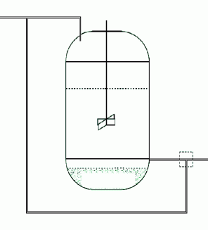
Figure 1: Schematics of a classical continuous stirred tank bioreactor with imperfect mixing corresponding to Cholette’s model.

Following the previous authors, we consider $\zeta_{f}$ as the manipulated variable (i.e. $\zeta_{f}=\emph{u}$) and let $\zeta$ be the controlled variable [4]. We are especially interested in the induced oscillatory behavior of the bioreactor. The common control law in this case is of the proportional integral type, that requires a dynamical error extension in order to build the closed-loop two dimensional system. Thus, the control law is given by

$$\emph{u}\triangleq\left(-K_{c}\cdot Error-K_{i}\int Error\,dt\right)~{},$$

where $K_{c}$ and $K_{i}$ are the control gain values. For the sake of simplicity, the closed-loop system is written as:

$$\dot{X} = -X\left(C+\frac{K_{1}}{(1+K_{2}X)^{2}}\right)+C\left(-{K_{c}}\left(X-{Ref}\right)-{K_{i}}Y\right)$$ (5)

$$\dot{Y} = X-Ref~{},$$ (6)

where

$$C=\frac{n\ F}{m\ V}~{},\ \ \ \ \ \ \ \ \ \ \ X=\zeta~{}.$$

Eq. (5) describes the dynamical behavior of the concentration, while Eq. (6) refers to the dynamical behavior of the integrated error.

3 Transformation to the Liénard form

In this section, we show that the system given by Eqs. (5-6) can be rewritten as a system of the form (2)-(3), i.e., in the Liénard generalized form. This is one of the main results of this work.

Proposition 1. Under the transformation

$$\left[\begin{array}[]{c}{x}\\ {y}\end{array}\right]=\Psi(X,Y)=\left[\begin{array}[]{c}{X-X_{p}}\\ {-Y+Y_{p}}\end{array}\right],$$ (11)

where

$$Y_{p} = -{\frac{{\it Ref}\,\left(C+K_{{1}}+{\it Ref}\,CK_{{2}}\left(K_{{2}}{\it Ref}+2\right)\right)}{C{\it K_{i}}\,\left(1+K_{{2}}{\it Ref}\right)^{2}}}$$

$$X_{p} = Ref,$$

system given by Eq. (5-6) can be written in the generalized Liénard form. With the following additional properties

• $g(0)=0$ and $xg(x)>0$ for $x\neq 0$;

• $\phi(0)=0$ and $\phi^{\prime}(x)>0$ for $a_{2}<y<b_{2}$;

• The curve $\phi(y)=F(x)$ is well defined for all $x\in(a_{1},b_{1})$.

Proof. If we substitute $X=x+X_{p}$ and $Y=-y+Y_{p}$ in Eqs. (5) and (6), and we choose

$$F(x) = x\left(C\left(1+{\it K_{c}}\right)+K_{{1}}\frac{\left(1-{\frac{K_{{2}}{\it Ref}\,\left(2+K_{{2}}\left(x+2\,{\it Ref}\right)\right)}{\left(1+K_{{2}}{\it Ref}\right)^{2}}}\right)}{\left(1+K_{{2}}\left(x+{\it Ref}\right)\right)^{2}}\right)$$ (12)

$$\phi(y) = C{\it K_{i}}\,y$$ (13)

$$g(x) = x~{},$$ (14)

we get the generalized Liénard form of the PI-controlled Cholette system. The properties [A1], [A2] and [A3] are straightforwardly checked in Eqs. (12)-(14).

For $\Psi(X,Y)$ to be a diffeomorphism on the region $\Omega$, it is necessary and sufficient that the Jacobian $\mathrm{d}\Psi(X,Y)$ be nonsingular on $\Omega$, and moreover that $\Psi(X,Y)$ is one to one from $\Omega$ to $\Psi(\Omega)$. Since $\Psi(X,Y)$ is linear, it is one to one and the determinant of the Jacobian matrix is constant, then is nonsingular in the region $\Omega=[-\infty,\infty]\times[-\infty,\infty]$.

In the literature, the properties [Ai] are standard properties assumed for Liénard systems [10]. We point out that the huge existing literature on Liénard systems deals mainly with cases in which $F(x)$ is polynomial [14], [12], [13], whereas we are in a case in which $F(x)$ is a nonlinear rational function. Such cases are far less studied and there are still many open problems.

4 Existence of Limit Cycles

We briefly recall some basic results of the theory of bifurcations of vector fields. Roughly speaking, a bifurcation is a change in equilibrium points, periodic orbits, or in their stability properties, when varying a parameter known as bifurcation parameter. The values of the parameter at which the changes occur are called bifurcation points. A Hopf bifurcation is characterized by a pair of complex conjugate eigenvalues crossing the imaginary axis. Now, suppose that the dynamical system $\dot{X}=f(X,\mu)$ with $X\in\mathbb{R}^{n}$ and $\mu\in\mathbb{R}$ has an equilibrium point at $X_{eq}$, for some $\mu={\mu}^{H}$; that is $f\left({X}_{eq},{\mu}^{H}\right)=0$. Let $A(\mu)=\frac{\partial f\left({X}^{H},{\mu}\right)}{\partial X}$ be the Jacobian matrix of the system at the equilibrium point. Assume that $A\left({\mu}^{H}\right)$ has as single pair of purely imaginary eigenvalues $S\left({\mu}^{H}\right)=\pm\dot{\imath}\omega_{H}$ with $\omega_{H}>0$ and that these eigenvalues are the only ones with the properties $\Re(S)=0$. If the following condition is fulfilled $\left.\frac{\mathrm{d}\Re\left(S(\mu)\right)}{\mathrm{d}\mu}\right|_{\mu=\mu^{H}}~{}\neq 0$ the Hopf bifurcation theorem states that at least one limit cycle is generated at $\left(X_{eq},\mu^{H}\right)$ (see [8]). The condition (4) is known as the transversality hypothesis. Considering now the $n$th degree characteristic polynomial $\lambda(S)=S^{n}+a_{1}S^{n-1}+a_{2}S^{n-2}+\ldots+a_{n}$, where all the real $a_{i}$ coefficients are positive allows the construction of a Hurwitz matrix $\mathcal{H}_{n\times n}$ Then one has the basic result that the characteristic polynomial is stable if and only if the leading principal minors of $\mathcal{H}_{n\times n}$ are all positive [9].

To search the Hopf bifurcation we have to calculate the equilibrium points of the system (2)-(3) making equal to zero the right-hand-side of the equation, and taking as bifurcation parameters the values of the PI-control gains. Then, finding the solution with respect to the state vector $x$ we notice that the closed-loop system has a unique equilibrium point located at the origin.

Proposition 2. If the parameter $K_{c}$ is such that

$$K_{c}^{H}-2\,{\frac{\sqrt{C{\it K_{i}}}}{C}}<{K_{c}}<K_{c}^{H}~{},$$

then the Liénard system (2) and (3) with the functions given in Eqs. (12)-(14) has at least one limit cycle. The upper limit $K_{c}^{H}$ is defined in Eq. (23).

Proof. If we use the Hurwitz criterion to guarantee that the unique equilibrium point is unstable, we evaluate the Jacobian of the system at the origin

$$\mathcal{J}\left(0,K_{c}\right)=\left[\begin{array}[]{cc}-C-{\frac{K_{{1}}}{\left(1+K_{{2}}{\it Ref}\right)^{2}}}+2\,{\frac{{\it Ref}\,K_{{2}}K_{{1}}}{\left(1+K_{{2}}{\it Ref}\right)^{3}}}-C{\it K_{c}}&C{\it K_{i}}\\ \vskip 6.0pt plus 2.0pt minus 2.0pt\cr-1&0\end{array}\right]~{}.$$ (17)

Then, from the determinant $IS-\mathcal{J}(0,K_{c})$, we get the characteristic polynomial $\lambda(S)={S}^{2}+{a_{1}}{S}+{a_{2}}$, where

$$a_{1} = C\left(1+{\it K_{c}}\right)-{\frac{K_{{1}}\left(K_{{2}}{\it Ref}-1\right)}{\left(1+K_{{2}}{\it Ref}\right)^{3}}}$$ (18)

$$a_{2} = {C}{K_{i}}~{}.$$ (19)

Then, the Hurwitz matrix is given by

$$\mathcal{H}=\left[\begin{array}[]{cc}{a_{1}}&{0}\\ {1}&{a_{2}}\end{array}\right]~{},$$ (22)

and its principal minors are $\mathcal{H}_{1}\left(K_{c}\right)={a_{1}}$ and $\mathcal{H}_{2}\left(K_{c}\right)={a_{1}}{a_{2}}$. From this formulas, we can note that the stability of the unique equilibrium point depends on the sign of Eq. (18). Since all the parameters in the Eqs. (18) and (19) are positive, we can induce the local stability as a function of the values of the controller gains involved in these equations and then we obtain the bifurcation point as the trivial solution of Eq. (18) for $K_{c}$ and restricting $K_{i}>0$

$${K_{c}}^{H}=-1+{\frac{K_{{1}}\left(K_{{2}}{\it Ref}-1\right)}{C\left(1+K_{{2}}{\it Ref}\right)^{3}}}~{}.$$ (23)

In order to test the transversality condition, the behavior of the eigenvalues of $\mathcal{J}(0,K_{c})$ in the neighborhood of $K_{c}^{H}$ should be analyzed. Thus, we take $K_{c}$ as $K_{c}^{H}+\epsilon$, with $\epsilon\in{\mathbb{R}}$. The transversality condition will be fulfilled if the sign of the equations $\mathcal{H}_{1}$ and $\mathcal{H}_{2}$ changes when the sign of $\epsilon$ changes. Substitution of Eq. (23) in the principal minor expressions gives $\mathcal{H}_{1}\left(K_{c}^{H}\right)={\epsilon}\left({C}\right)$ and $\mathcal{H}_{2}\left(K_{c}^{H}\right)={\epsilon}\left({K_{i}}{C}^{2}\right)$.

From the above equations we can appreciate that if we want to have a positive real part of the eigenvalues of the Jacobian matrix (17), we need that $\epsilon$ be negative. In other words, it is below the value given by Eq. (23) where the limit cycles are generated. Using $K_{c}^{H}$, the eigenvalues of the matrix (17) are given by the roots of the characteristic polynomial $\lambda(S)$, which are

$$S_{1} = -\frac{\epsilon\,C}{2}+\frac{\sqrt{{\epsilon}^{2}{C}^{2}-4\,C{\it K_{i}}}}{2}$$ (24)

$$S_{2} = -\frac{\epsilon\,C}{2}-\frac{\sqrt{{\epsilon}^{2}{C}^{2}-4\,C{\it K_{i}}}}{2}~{},$$ (25)

where we can notice that the eigenvalues are complex with positive real parts, when $0>\epsilon>-2\,{\frac{\sqrt{C{\it K_{i}}}}{C}}$ and $K_{i}>0$.

Eq. (23) is of main importance, because it corresponds to the Hopf bifurcation and therefore lies in a neighborhood of the value of the parameter where at least one limit cycle is generated. Note, that the Hopf bifurcation by itself can not guarantee the uniqueness of the limit cycle, because more than one limits cycle could appear [7]. Then we need to use additional constraints in order to find the condition for uniqueness.

5 Uniqueness of Limit Cycles

Xiao and Zhang [10] gave an interesting theorem on the uniqueness of limit cycles for generalized Liénard systems, under the conditions [A1], [A2] and [A3] that allows us to prove a novel property of PI-controlled Cholette bioreactors.

Theorem 1. Using the notations $G(x)=\int_{0}^{x}g(x)dx$ and $f(x)=F^{{}^{\prime}}(x)$, suppose that the system (2) - (3) satisfies the following conditions:

• there exist $x_{1}$ and $x_{2}$, $a_{1}<x_{2}<0<x_{1}<b_{1}$ such that $F(x_{1})=F(0)=0$, $F(x_{2})>0$ and $G(x_{2})\leq G(x_{1})$; $xF(x)\leq 0$ for $x_{2}\leq x\leq x_{1}$, $F^{\prime}(x)>0$ for $a_{1}<x<x_{2}$ or $x_{1}<x<b_{1}$, and $F(x)\neq 0$ for $0<\mid x\mid\ll 1$.

• $F(x)f(x)/g(x)$ is nondecreasing for $x_{1}<x<b_{1}$.

• $\phi^{\prime}(y)$ is nonincreasing as $\mid y\mid$ increases.

Then the system (2) and (3) has at most one limit cycle, and it is stable if it exists.

Note that the above result does not guarantee the existence of limit cycles by itself.

Proposition 3. System (2) and (3) with the functions given by the Eqs.  (12)-(14) and with $Ref>{2}/{K_{2}}$ and $K_{c}={K_{c}}^{H}+\epsilon^{\ast}$, where

$$\epsilon^{\ast}=-\,{\frac{K_{{1}}\left(-2+K_{{2}}{\it Ref}\right)}{2C\left(1+K_{{2}}{\it Ref}\right)^{3}}}~{},$$ (26)

has a unique limit cycle.

Proof. The existence is given by the Proposition 2, and the uniqueness will be proved by showing that the system fulfills the conditions of Theorem 1. Let us take $Ref^{\ast}={2\kappa}/{K_{2}}$ with $\kappa>1$ which agrees with the condition stated in Proposition 3. Then

$${K_{c}}^{H}(\epsilon^{\ast},Ref^{\ast})=-1+{\frac{K_{{1}}\kappa}{C\left(1+2\,\kappa\right)^{3}}}~{}.$$

For these values of the parameters, the function $F(x)$ is simplified to the form

$$F^{\ast}(x)={\frac{xK_{{1}}\left(3\,\kappa+\kappa\,{K_{{2}}}^{2}{x}^{2}-4\,{\kappa}^{3}+1\right)}{\left(1+2\,\kappa\right)^{3}\left(1+K_{{2}}x+2\,\kappa\right)^{2}}}~{}.$$ (27)

The real roots of $F^{\ast}(x)$ are $0$, $x_{1}$, and $-x_{1}$, where

$$x_{1}={\frac{\sqrt{\kappa\,\left(-1+\kappa\right)}\left(1+2\,\kappa\right)}{\kappa\,K_{{2}}}}~{},$$

which fulfill the property $F(x_{1})=F(0)=0$. Moreover, taking $x_{2}=-\xi x_{1}$, where $0<\xi<1$, one can see that $x_{2}<0<x_{1}$. To evaluate $F^{\ast}(x)$ in the intervals $x_{2}<x<0$ and $0<x<x_{1}$, it is sufficient to substitute in Eq. (27) $x=\beta\,x_{i}$, where $i=1,2$ and $0<\beta<1$. Then we can easily verify that

$$0>F^{\ast}(\beta\,x_{1}) = {\frac{\left(-1+\kappa\right)\left(\beta^{2}-1\right)\kappa\,K_{{1}}\beta\,\sqrt{\kappa\,\left(-1+\kappa\right)}}{\left(1+2\,\kappa\right)^{2}\left(\kappa+\beta\,\sqrt{\kappa\,\left(-1+\kappa\right)}\right)^{2}K_{{2}}}}$$ (28)

$$0<F^{\ast}(\beta\,x_{2}) = -\xi{\frac{\left(-1+\kappa\right)\left(\beta^{2}\,-1\right)\kappa\,K_{{1}}\,\beta\,\sqrt{\kappa\,\left(-1+\kappa\right)}}{\left(1+2\,\kappa\right)^{2}\left(-\kappa+\,\beta\,\sqrt{\kappa\,\left(-1+\kappa\right)}\right)^{2}K_{{2}}}}~{}.$$ (29)

Consequently, $xF^{\ast}(x)\leq 0$ for $x_{2}\leq x\leq x_{1}$. Moreover, $G(x)=x^{2}/2$ and then $G(x_{2})\leq G(x_{1})$. Besides, for $\theta>1$ we have

$$0<F^{\ast^{\prime}}({\theta}{x_{1}})={\frac{\left(-1+\kappa\right)\left((-1+3\,{\theta}^{2})\kappa+(\theta+\theta^{3})\sqrt{\kappa\,\left(-1+\kappa\right)}\right)K_{{1}}{\kappa}^{2}}{\left(1+2\,\kappa\right)^{3}\left(\kappa+\theta\sqrt{\kappa\,\left(-1+\kappa\right)}\right)^{3}}}~{}.$$

In other words, $F^{\ast^{\prime}}(x)>0$ for $x_{1}<x<b_{1}$. From Eq. (12) we can see that $F^{\ast}(x)\neq 0$ for $0<\mid x\mid\ll 1$. In addition, since $\phi^{\prime}(y)=CK_{i}$, no matter how $\mid y\mid$ increases, $\phi^{\prime}(y)$ remains constant. Finally, we can write $\Psi(x)\equiv F^{\ast}(x)f(x)/g(x)=(\mathcal{A}+\mathcal{B})/\mathcal{C}$, where

$$\mathcal{A} = 2+\kappa\,\left(16\,{\kappa}^{2}+{K_{{2}}}^{3}{x}^{3}\right)-\kappa\,\left(1+2\,\kappa\right)\left(xK_{{2}}\left(3\,K_{{2}}x+8\,\kappa+4\right)-12\right)$$ (30)

$$\mathcal{B} = 2\,\ln\left(1+K_{{2}}x+2\,\kappa\right)\left(1+2\,\kappa\right)^{3}\left(1+K_{{2}}x+2\,\kappa\right)$$ (31)

$$\mathcal{C} = {\frac{{K_{{1}}}^{2}}{2\left(1+2\,\kappa\right)^{6}{K_{{2}}}^{2}\left(1+K_{{2}}x+2\,\kappa\right)^{3}}}~{}.$$ (32)

Performing the derivative of $\Psi(x)$, evaluating it at $x={x_{1}}{\alpha}$ for $\alpha>1$, and plotting $\vartheta\Psi^{\prime}({x_{1}}{\alpha})$, where

$$\vartheta={\frac{\left(1+2\,\kappa\right)^{5}\left(\kappa+\alpha\,\sqrt{\kappa\,\left(-1+\kappa\right)}\right)^{4}K_{{2}}}{{K_{{1}}}^{2}{\kappa}^{3}}}~{},$$ (33)

we get the positive function displayed in Fig. 2. Thus, $F^{\ast}(x)f(x)/g(x)$ is nondecreasing for $x_{1}<x<b_{1}$. In this way, we checked each of the three conditions of Theorem 1. The unique limit cycle can be seen in Fig. 3 that illustrates the numerical simulation corresponding to the results obtained until now.

6 Case Study

With the aim of illustrate the results given in the previous sections, we perform numerical simulation using the values of the parameters given by Chidambaram [5]. All our calculations are performed for a flow characterized by the value of the Damköhler number $(Da=K_{1}V/F)$ equal to 300, as reported by Sree and Chidambaram [4].

Table 2: The values of the parameters of Cholette’s model [4].

Symbol	Value	Units
$F$	$3.333\times 10^{-5}$	$[m^{3}/s]$
$V$	$10^{-3}$	$[m^{3}]$
$K_{1}$	$10$	$[1/s]$
$K_{2}$	$10$	$[m^{3}/Kmol]$
$n$	$0.75$	$[$dimensionless $]$
$m$	$0.75$	$[$dimensionless $]$

In Fig. 4 a plot of the evolution in time of the variable $x$ is given for two values of the integral parameter $K_{i}$. It indicates that the oscillation frequency can be manipulated through this control parameter.

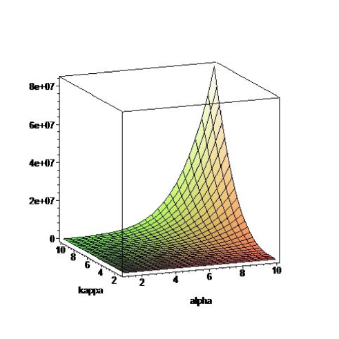
Figure 2: The function $\vartheta\Psi^{\prime}(\alpha x_{1})$, for $\alpha>1$, and $\kappa>1$. We see that this is a strictly positive function.

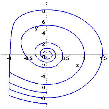
Figure 3: The phase portrait of the PI-controlled Cholette model subjected to the uniqueness conditions. The employed values of the parameters are those given in Table 1.

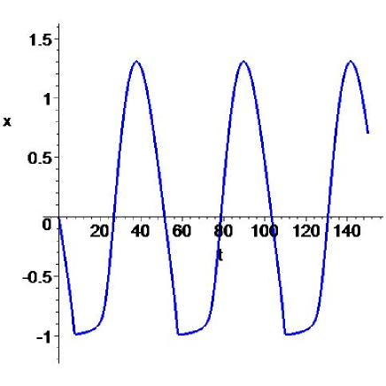
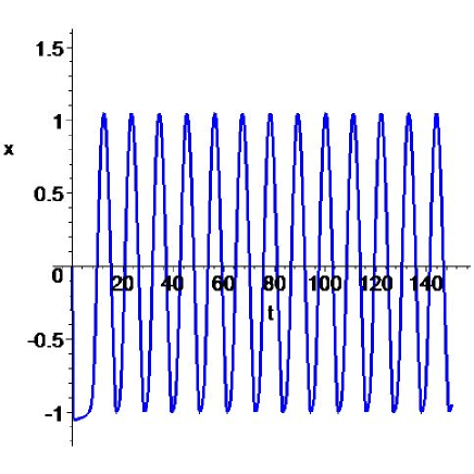
Figure 4: Time evolution of the variable $x$. The left hand side plot corresponds to $K_{i}=0.5$, while the right hand side plot corresponds to $K_{i}=10$. This is a graphical representation of the fact that oscillation frequency is a function of the control gain parameter $K_{i}$.

7 A Local Center of the Generalized Liénard System ?

We begin this section by recalling that a limit cycle is an isolated closed orbit, while a critical point is a center if all orbits in its neighborhood are closed. To the best of our knowledge the literature on period annuli for Liénard systems is well developed only for polynomial cases and moreover it focuses on Hamiltonian type systems [11], [15], [16].

Notice that for $K_{c}(Ref^{\ast})=K_{c}^{H}(Ref^{\ast})+\epsilon$ and $\epsilon$ in the following interval $\epsilon^{\ast}<\epsilon<0$ the existence of limit cycles is proved but without guaranteeing uniqueness. It is precisely in this interval where our numerical simulations point to the existence of a local center in a neighborhood of the origin. Fig. 5 shows the phase portrait of the PI-controlled generalized Liénard system with a value of $K_{c}$ in the same interval and close to $K_{c}^{H}$.

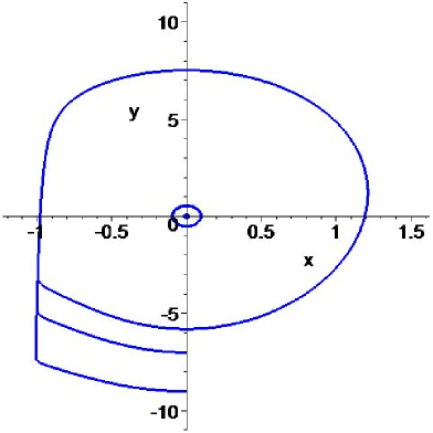
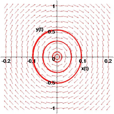
Figure 5: The phase portrait of the PI-controlled generalized Liénard system with a value of $K_{c}^{H}(Ref^{\ast})+\epsilon$ in the interval $\epsilon^{\ast}<\epsilon<0$ and close to $K_{c}^{H}$. The upper plot shows the state space with the limit cycle and the possible annulus in the neighborhood of the origin, while the lower plot displays the configuration of the vector field close to the origin.

8 Conclusions

The main result of this paper is that the Cholette CSTR model under PI control can be mapped into a generalized Liénard dynamical system of nonpolynomial type. Thus, we establish a new important application of this class of nonlinear oscillators that allows us to make a detailed study of the oscillatory dynamical behavior of these interesting bioreactors.

Sufficient conditions for the existence and uniqueness of limit cycles of this generalized Liénard system are stated in this paper together with numerical simulations that indicate the possibility of the existence of a local center (period annulus) when the gain proportional parameter $K_{c}$ of the control law is close to the value $K_{c}^{H}$ corresponding to the existence condition of limit cycles. We also notice that the oscillation frequency is a function of the integral control gain parameter $K_{i}$, a result that could have practical applications. We mention that similar results have been obtained by Albarakati, Lloyd, & Pearson [17] for the polynomial case.

Our work also shows that the Liénard representation of dynamical systems and its associated results could have a remarkable potential as an effective tool in the control theory for the closed-loop dynamical analysis in the plane.

References

- [1] Lo, S.N., & Cholette, A., (1983). Multiplicity of a conversion in cascade in imperfectly stirred tank reactors. Chem. Eng. Sci. 38, 367.
- [2] Liou, C.T., & Y.S. Chien, (1991). The effect of nonideal mixing on input multiplicity in a CSTR. Chem. Eng. Sci. 46, 2113.
- [3] Sree, R.P., & Chidambaram, M.A., (2002). Identification of unstable transfer model with a zero by optimization method. J. Indian Inst. Sci. 82, 219.
- [4] Sree, R.P., & Chidambaram, M.A., (2003). Control of unstable bioreactor with dominant unstable zero. Chem. Biochem. Eng. Q. 17, 139.
- [5] Sree, R.P., & Chidambaram, M.A., (2003). A simple method of tuning PI controllers for unstable systems with a zero. Chem. Biochem. Eng. Q. 17, 207.
- [6] Kumar, V.R., & Kulkarni, B.D., (1994). On the operation of a bistable CSTR: a strategy employing stochastic resonance, Chem. Eng. Sci. 49, 2709.
-
[7]
Gaiko, V.A., (2000). Global bifurcations of limit cycles,
http://www.neva.ru/journal, Diff. Eqs. and Control Processes, No. 3, 1. - [8] Gordillo, F., Salas, F., Ortega, R., Aracil, J., (2002). Hopf bifurcation in indirect field-oriented control of induction motors, Automatica 38, 829.
- [9] Ogata, K., (2001). Modern Control Engineering, 4th edition, Prentice Hall.
- [10] Xiao D., & Zhang, Z., (2000). On the uniqueness and nonexistence of limit cycles for predator-prey systems., Nonlinearity 16, 1.
- [11] Li, W., Llibre, J., & Zhang, X., (2004). Melnikov functions for period annulus, nondegenerate centers, heteroclinic and monoclinic cycles. Pacific J. Math. 213, 49.
- [12] Giacomini, H., & Neukirch, S., (1997). Number of limit cycles of the Liénard equation. Phys. Rev. E 56, 3809.
- [13] Giacomini, H., & Neukirch, S., (1997). Improving a method for the study of limit cycles of the Liénard equation. Phys. Rev. E 57, 6573.
- [14] Giacomini, H., & Neukirch, S., (1998). Algebraic approximations to bifurcation curves of limit cycles for the Liénard equation. Phys. Lett. A 244, 53.
- [15] Du, Z., (2004). On the critical periods of Liénard systems with cubic restoring forces. Int. J. Math. and Math. Sci. 61, 3259.
- [16] Cristopher, C.J., & Devlin, J., (1997). Isochronous center in planar polynomial systems SIAM J. Math. Anal. 28, 162.
- [17] Albarakati, W.A., Lloyd, N.G., & Pearson J.M., (2000). Transformation to Liénard form. Electronic J. Diff. Eqs., Vol. 2000, No. 76, 1.