A Weakly Nonlinear Analysis of Impulsively–Forced Faraday Waves

Abstract

Parametrically-excited surface waves, forced by a repeating sequence of $N$ delta-function impulses, are considered within the framework of the Zhang-Viñals model Zhang and Viñals (1997). The exact impulsive-forcing results, in the linear and weakly nonlinear regimes, are compared with results obtained numerically for sinusoidal and multifrequency forcing. We find surprisingly good agreement between impulsive forcing results and those obtained using a two-term truncated Fourier series representation of the impulsive forcing function. With impulsive forcing, the linear stability analysis can be carried out exactly and leads to an implicit equation for the neutral stability curve. As noted previously by Bechhoefer and Johnson Bechhoefer and Johnson (1996), in the simplest case of $N=2$ equally-spaced impulses per period (which alternate up and down) there are only subharmonic modes of instability. The familiar situation of alternating subharmonic and harmonic resonance tongues emerges only if an asymmetry in the spacing between the impulses is introduced. We extend the linear analysis for $N=2$ impulses per period to the weakly nonlinear regime, where we determine the leading order nonlinear saturation of one-dimensional standing waves as a function of forcing strength. Specifically, an analytic expression for the cubic Landau coefficient in the bifurcation equation is derived as a function of the dimensionless spacing between the two impulses and the fluid parameters that appear in the Zhang-Viñals model. As the capillary parameter is varied, one finds a parameter region of wave amplitude suppression, which is due to a familiar 1:2 spatio-temporal resonance between the subharmonic mode of instability and a damped harmonic mode. This resonance occurs for impulsive forcing even when harmonic resonance tongues are absent from the neutral stability curve. The strength of this resonance feature can be tuned by varying the spacing between the impulses. This finding is interpreted in terms of a recent symmetry-based analysis of multifrequency forced Faraday waves Porter et al. (2004); Topaz et al. (2004).

I I. Introduction

Standing waves form spontaneously on the free surface of a fluid layer when it is subjected to a time-periodic vertical vibration of sufficient strength. The waves, which result from a symmetry-breaking parametric instability, organize themselves into remarkably regular patterns, as first described by Faraday in 1831 Faraday (1831). In modern experiments, a variety of container geometries, fluids and forcing functions have been employed, resulting in a rich variety of standing wave patterns, as well as a range of dynamical responses. See Miles and Henderson (1990); Müller et al. (Springer, 1998) for reviews on Faraday waves. In this paper, we investigate the response of the Faraday system to an idealized forcing function consisting of a periodic sequence of delta-function impulses. The results are contrasted with those obtained in the classical cases of single and multifrequency forcing.

The versatility of the Faraday system for investigating pattern formation owes much to the vastness of its control parameter space. By varying the forcing frequency and amplitude, as well as the fluid properties, experimentalists employing a sinusoidal acceleration function have teased out spatially regular patterns ranging from stripes, hexagons and squares to targets, spirals and quasipatterns Christiansen et al. (1992); Kudrolli and Gollub (1996); Binks and van der Water (1997); Wagner et al. (2000). The seminal experiments of Edwards and Fauve Edwards and Fauve (1994) showed how the addition of a second commensurate frequency component in the forcing function could lead to even greater versatility of this system, via the controlled introduction of additional length scales. Two-frequency forcing has led to a variety of exotic superlattice patterns Kudrolli et al. (1998); Arbell and Fineberg (1998), as well as quasipatterns Edwards and Fauve (1993); Arbell and Fineberg (2000a), triangular patterns Müller (1993) and localized structures Arbell and Fineberg (2000b). A detailed description of patterns readily achieved in two-frequency Faraday experiments can be found in Arbell and Fineberg (2002). Recent experiments by Epstein and Fineberg Epstein and Fineberg (2004) have shown how a third perturbing frequency can be used to rapidly switch between the novel patterns achieved with two-frequency forcing.

Theoretically, the Faraday system presents a number of challenges due both to the explicit time-dependence of the forcing and the free-boundary nature of the problem; for a partial review of theoretical work see Müller et al. (Springer, 1998). Consequently, models incorporating simplifying assumptions have often been relied on, in conjunction with numerical linear stability analysis or perturbative methods. In this manner, much has been accomplished. Linear stability results build on the classic paper of Benjamin and Ursell Benjamin and Ursell (1954), who explained Faraday’s observation of a subharmonic response of the fluid layer to sinusoidal forcing. Specifically, they showed that the linear stability problem, in the case of an ideal fluid, reduces to a Mathieu equation, for which the natural frequency of oscillation is given by the inviscid dispersion relation. Subsequent investigators carried out linear stability analyses on the full fluid problem with sinusoidal forcing Kumar and Tuckerman (1994); Beyer and Friedrich (1995); Kumar (1996); Chen and Viñals (1997). These results were also extended to two-frequency forcing in Besson et al. (1996). Theoretical understanding of the nonlinear problem progressed with the introduction of a quasipotential formulation of the Faraday wave problem by Zhang and Viñals Zhang and Viñals (1997). This model, which describes small amplitude surface waves on a semi-infinite, weakly viscous fluid layer, eliminates the bulk flow, assumed to be potential, from the description. The free boundary $z=h({\bf x},t)$ $({\bf x}\in\mathbb{R}^{2})$ is then prescribed by an evolution equation for $h$, which is coupled to an evolution equation for a surface velocity potential $\Phi$; see Section II. Zhang and Viñals used this model to further investigate nonlinear effects via an asymptotic expansion, which demonstrated the importance of resonant triads (three-wave resonance) in the pattern selection process. Later, Chen and Viñals Chen and Viñals (1999) used perturbation methods to derive amplitude equations directly from the Navier-Stokes equations assuming only that the depth of the fluid layer is (effectively) infinite. These approaches yield good agreement with experiments in the relevant parameter regimes, but typically require a numerical evaluation of relevant quantities to make the comparison.

An alternative theoretical approach to the Faraday wave pattern selection problem is based in equivariant bifurcation theory Golubitsky et al. (1988); Crawford and Knobloch (1991). This “model-independent” treatment of the symmetry-breaking bifurcations relevant to the Faraday experiment has proved especially fruitful in analyzing spatially-periodic superlattice patterns Silber and Proctor (1998); Tse et al. (2000). An extension of this approach, tailored to the multifrequency Faraday problem, uses spatio-temporal symmetry arguments to derive amplitude equations based on the patterns’ symmetries. The form of the coefficients in the equations reflect the temporal (parameter) symmetries of the forcing function and the time-reversal symmetry that is broken by the damping. The equations describe not only the critical modes, but also certain damped modes that are nonlinearly driven by them. These studies reveal the role of the various forcing parameters (frequencies, amplitudes, and relative phases) in nonlinearly coupling the driven modes to key weakly-damped modes. The results give insight into the pattern selection process and can be used to explain a number of characteristics of the experimentally observed patterns Silber and Skeldon (1999); Topaz and Silber (2002); Porter and Silber (2004); Porter et al. (2004); Topaz et al. (2004).

The investigations reviewed above focus on Faraday waves parametrically-excited by sinusoidal and multifrequency forcing functions. An alternative forcing function, consisting of a periodic sequence of delta-function impulses, was proposed by Bechhoefer and Johnson Bechhoefer and Johnson (1996) who indicated how the linear analysis could be greatly simplified in this case. (This idealization of parametrically forced systems has been put forth in a variety of physical contexts; see, for example, Hsu (1972); Hsu and Cheng (1973); Pilipchuk et al. (1999).) Recently, Huepe and Silber Huepe and Silber (in prep.) showed that the linear analysis of the impulsively-forced Faraday problem for a viscous fluid, as proposed in Bechhoefer and Johnson (1996), breaks down in certain parameter regimes. In these regimes, the flow in the fluid bulk cannot be (instantaneously) matched across the delta impulses. However, these complications are absent from the Zhang-Viñals formulation, which describes the evolution of the free surface, with the bulk flow eliminated from the model. In this paper we extend the results of Bechhoefer and Johnson on impulsively-forced Faraday waves into the weakly nonlinear regime, within the framework of the Zhang-Viñals model.

Following the method of Hsu (1972), we develop a simple modular approach to constructing the stroboscopic map associated with the linear stability problem. Specifically, we construct the linear maps which evolve perturbations of wavenumber $k$ from one impulse in the sequence to the next. The linear map associated with one period of the forcing is then obtained by multiplication of $N$ matrices, one for each impulse in the periodic sequence. From this simple construction we can derive explicit expressions for the Floquet multipliers associated with the linear stability problem, and arrive at an equation (implicit if $N>2$) that describes the neutral stability curve. We analyse the results in the simplest case of $N=2$ impulses in detail, and compare them with those obtained with an $M$-term truncated Fourier series representation of the impulsive forcing function. While the neutral stability curves are poorly approximated by the truncated Fourier series even for very large $M$, the onset parameters of critical forcing strength and wavenumber are quite accurately determined with a single-term sinusoidal approximation (i.e., for $M=1$).

We extend the analysis for $N=2$ impulses per period to the weakly nonlinear regime for one-dimensional surface waves. A key observation of Bechhoefer and Johnson Bechhoefer and Johnson (1996) is that there are no harmonic resonance tongues for a sequence of $N=2$ impulses if they are equally spaced in time (i.e., an up impulse and then a down impulse half a period later). We show that, despite the absence of harmonic instabilities, there can still be a resonant interaction between the excited subharmonic and damped harmonic modes which leads, in one dimension, to an associated degradation in the nonlinear response of the fluid to the vibration in the weakly nonlinear regime. This is similar to the spatio-temporal 1:2 resonance that occurs in the case of sinusoidal forcing Zhang and Viñals (1997), for which subharmonic and harmonic instabilities alternate with increasing perturbation wavenumber $k$. Thus, although the harmonic modes can never be linearly excited in this particular impulsive case, these modes can nonetheless be driven nonlinearly by the critical subharmonic modes and in this way influence the nonlinear evolution of the instability. In addition to analysing the case of $N=2$ equally-spaced impulses, we explore the effects of varying the spacing between the impulses so that they are no longer exactly half a period apart. We find that this asymmetry in impulse timing enhances or diminishes the influence of the 1:2 resonance on the standing wave amplitude depending on the sense in which it is applied. We understand this result by considering a two-term Fourier series approximation to the impulsive forcing function, and applying recent results pertaining to multifrequency forcing Porter et al. (2004); Topaz et al. (2004).

Our paper is organized as follows. In the next section we present the Zhang-Viñals model of Faraday waves, and then carry out the linear stability analysis in the general case of $N$ impulses per forcing period. We then focus on the simplest case of $N=2$ and examine in detail the sequence of subharmonic and harmonic resonance tongues as a function of the dimensionless spacing between the impulses. We compare our results with those obtained with sinusoidal and multifrequency forcing functions within the context of a truncated Fourier series representation of the impulsive forcing function. In section III we derive the cubic bifurcation equation that determines the amplitude of one-dimensional spatially-periodic surface waves driven by impulsive forcing, focusing on the 1:2 spatio-temporal resonance feature. We compare our weakly nonlinear results with those obtained with single and two-frequency forced Faraday waves. Finally, in Section IV, we summarize our results and indicate some promising directions for subsequent investigations.

II Linear results for the Zhang-Viñals Faraday wave model

This section introduces the Zhang-Viñals model for Faraday waves. A linear stability analysis is then performed for waves excited by a periodic sequence of $N$ impulses and detailed results are presented for the simplest case of $N=2$.

II.1 Zhang-Viñals model

The quasipotential formulation of the Faraday wave problem, due to Zhang and Viñals Zhang and Viñals (1997), is derived from the Navier-Stokes equations assuming small amplitude surface waves on a deep, nearly inviscid fluid layer. It describes the free surface height $h(\textbf{x},t)$ and surface velocity potential $\Phi(\textbf{x},t)$ of a fluid subjected to a (dimensionless) periodic vertical acceleration function $G(t)$. Employing these equations greatly simplifies our calculations since the flow in the bulk does not appear explicitly — we need only track the behavior of the free surface, a function of the horizontal coordinate $\textbf{x}\in\mathbb{R}^{2}$ and time $t$. The Zhang-Viñals model takes the form

$$(\partial_{t}-\gamma\nabla^{2})h-\hat{D}\Phi =N_{1}(h,\Phi),$$ (1a)

$$(\partial_{t}-\gamma\nabla^{2})\Phi-(\Gamma_{0}\nabla^{2}-G_{0}+G(t))h =N_{2}(h,\Phi),$$ (1b)

where the nonlinear terms in (1) are given by

$$N_{1}(h,\Phi)= \;-\nabla\cdot(h\nabla\Phi)+{1\over 2}\nabla^{2}(h^{2}\hat{D}\Phi)-\hat{D}(h\hat{D}\Phi)$$

$$+\hat{D}(h\hat{D}(h\hat{D}\Phi)+{1\over 2}h^{2}\nabla^{2}\Phi),$$ (2a)

$$N_{2}(h,\Phi)= \;\frac{1}{2}(\hat{D}\Phi)^{2}-\frac{1}{2}(\nabla\Phi)^{2}-{1\over 2}\Gamma_{0}\nabla\cdot((\nabla h)(\nabla h)^{2})$$

$$-(\hat{D}\Phi)(h\nabla^{2}\Phi+\hat{D}(h\hat{D}\Phi)).$$ (2b)

Here the operator $\hat{D}$ multiplies each Fourier component by its wavenumber, e.g. $\hat{D}e^{i\textbf{k}\cdot\textbf{x}}=|\textbf{k}|e^{i\textbf{k}\cdot\textbf{x}}$, and the dimensionless fluid parameters are

$$\gamma\equiv\frac{2\nu k_{0}^{2}}{\omega},\quad\Gamma_{0}\equiv\frac{\Gamma k_{0}^{3}}{\rho\omega^{2}},\quad G_{0}\equiv\frac{gk_{0}}{\omega^{2}},$$ (3)

where $g$ is the usual gravitational acceleration, $\omega$ is the forcing frequency ($2\pi$ divided by the forcing period), $\nu$ is the kinematic viscosity, $\rho$ is the density, and $\Gamma$ is the surface tension. The wavenumber $k_{0}$ is chosen to satisfy the inviscid dispersion relation

$$gk_{0}+\frac{\Gamma k_{0}^{3}}{\rho}=\left(\frac{\omega}{2}\right)^{2},$$ (4)

where $\frac{\omega}{2}$ is the frequency associated with the typical subharmonic response of Faraday waves. After dividing (4) by $\omega^{2}$ we find $G_{0}+\Gamma_{0}=\frac{1}{4}$. $G(t)$ describes the applied acceleration; since time has been scaled by the forcing frequency $\omega$, the dimensionless period of $G(t)$ is $2\pi$.

We write the impulsive forcing function in the form

$$G_{imp}(t)=\sum_{n=-\infty}^{\infty}f_{n}\delta(t-t_{n})\ .$$ (5)

It is parameterized by the locations $t_{n}$ of the impulses ($t_{n}<t_{n+1}$, $t_{n+N}-t_{n}=2\pi$) and by the amplitudes $f_{n}$ ($f_{n+N}=f_{n}$), where $N$ is the number of impulses in the repeating sequence. The dimensionless amplitude $f_{n}$ of an impulse is given by

$$f_{n}\equiv\frac{v_{n}k_{0}}{\omega},$$ (6)

where $v_{n}$ is the jump in velocity at time $t_{n}$. We must also require

$$\sum_{n=1}^{N}f_{n}=0,$$ (7)

to prevent a net translation of the container (for suitably chosen initial velocity). An example of an impulsive acceleration function, along with the corresponding velocity and position functions, is shown in Fig. 1.

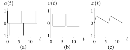
Figure 1: Example of (a) acceleration, (b) velocity, and (c) position of the fluid container over time in the case of two impulses per period. The positions of the vertical lines in the acceleration function denote the locations of the delta functions; here they have equal magnitude.

II.2 Linear stability analysis

II.2.1 Calculations

Our linear stability calculations follow the method of Bechhoefer and Johnson (1996). From (1), the linear stability problem takes the form

$$\left[(\partial_{t}-\gamma\nabla^{2})^{2}\!-\!\hat{D}(\Gamma_{0}\nabla^{2}\!-\!(G_{0}\!-\!G(t)))\right]h(x,t)=0.$$ (8)

We then write $h({\bf x},t)=p_{k}(t)e^{i{\bf k}\cdot{\bf x}}+c.c.$, where $c.c.$ denotes complex conjugate, and find that $p_{k}(t)$ satisfies

$$p_{k}^{\prime\prime}+2\gamma k^{2}p_{k}^{\prime}+[\gamma^{2}k^{4}+\Gamma_{0}k^{3}+(G_{0}-G(t))k]p_{k}=0,$$ (9)

where the prime denotes differentiation with respect to $t$ and the $k$ subscript emphasizes the dependence of the solution on the perturbation wavenumber $k=|{\bf k}|$. Hereafter we focus on $k\neq 0$; the $k=0$ mode cannot be excited due to mass conservation. (This is reflected in the governing equations (2) through the spatial derivatives in the nonlinear terms which ensure that the $k=0$ mode decouples from the other modes.)

Between each impulse, (9) is simply the equation for a damped harmonic oscillator, with solution

$$p_{k}(t)=A_{k,n}e^{(-\gamma k^{2}+i\omega_{k})(t-t_{n})}+c.c.,\>\>\>\>t\in(t_{n},t_{n+1}).$$ (10)

Here $\omega_{k}$ is the natural frequency of a wave with wavenumber $k$, which is determined by the dispersion relation

$$\omega_{k}^{2}=\Gamma_{0}k^{3}+G_{0}k.$$ (11)

We demand that $p_{k}(t)$ be continuous across each impulse, i.e., $p_{k}(t_{n}^{+})=p_{k}(t_{n}^{-})\equiv p_{k}(t_{n})$, where $p_{k}(t_{n}^{\pm})\equiv\lim_{t\rightarrow t_{n}^{\pm}}p_{k}(t)$. Integrating (9) across the $n^{th}$ impulse we obtain the following jump condition:

$$p_{k}^{\prime}(t_{n}^{+})-p_{k}^{\prime}(t_{n}^{-})=f_{n}k\,p_{k}(t_{n}).$$ (12)

This condition, together with the continuity requirement, yields the following map from $A_{k,n}$ to $A_{k,n+1}$:

$$\left(\begin{array}[]{c}A_{k,n+1}^{r}\\ A_{k,n+1}^{i}\end{array}\right)=e^{-\gamma k^{2}d_{n}}M_{k,n}\left(\begin{array}[]{c}A_{k,n}^{r}\\ A_{k,n}^{i}\end{array}\right),$$ (13)

where

$$M_{k,n}\equiv\left(\begin{array}[]{cc}c_{k,n}&-s_{k,n}\\ s_{k,n}-F_{k,n+1}c_{k,n}&c_{k,n}+F_{k,n+1}s_{k,n}\end{array}\right).$$ (14)

Here $A_{k,n}^{r}$ ($A_{k,n}^{i}$) is the real (imaginary) part of $A_{k,n}$ and $c_{k,n}\equiv\cos(\omega_{k}d_{n})$, $s_{k,n}\equiv\sin(\omega_{k}d_{n})$, $F_{k,n}\equiv\frac{f_{n}k}{\omega_{k}}$. Note that (14) depends on only two parameters: $d_{n}\equiv t_{n+1}-t_{n}$, the time between the $n^{th}$ and $(n+1)^{st}$ impulses, and $f_{n+1}$, the strength of the $(n+1)^{st}$ impulse.

Piecing together the relationships between $A_{n}$ and $A_{n+1}$, $A_{n+1}$ and $A_{n+2}$, etc. across one period, we find the stroboscopic map that relates the solution of the linearized problem at time $t_{n}$ to the solution one period later (i.e., after the sequence of $N$ impulses):

$$\left(\begin{array}[]{c}A_{k,n+N}^{r}\\ A_{k,n+N}^{i}\end{array}\right)=e^{-2\pi\gamma k^{2}}M_{k}\left(\begin{array}[]{c}A_{k,n}^{r}\\ A_{k,n}^{i}\end{array}\right).$$ (15)

Here $M_{k}\equiv M_{k,n+N-1}\cdots M_{k,n}$, where $M_{k,j}$ is given by (14).

The eigenvalues of $e^{-2\pi\gamma k^{2}}M_{k}$ determine the linear stability of the interface to disturbances of wavenumber $k$. Note that $M_{k}$ has determinant one, so these eigenvalues ($\lambda_{\pm}$) can be related to the trace of $M_{k}$ by $e^{2\pi\gamma k^{2}}\lambda_{\pm}=\frac{1}{2}{\rm Tr}(M_{k})\pm\sqrt{(\frac{1}{2}{\rm Tr}(M_{k}))^{2}-1}$. An instability exists when both eigenvalues (Floquet multipliers) are real and the magnitude of one exceeds unity. The threshold condition is therefore

$$\frac{1}{2}{\rm Tr}(M_{k})=\pm\cosh(2\pi\gamma k^{2}),$$ (16)

where ‘+’ corresponds to the harmonic case (Floquet multiplier $+1$), and ‘$-$’ corresponds to the subharmonic case (Floquet multiplier $-1$). This threshold condition defines an implicit equation for the neutral stability curve $f(k)$, where $f$ is an appropriate measure of the overall impulse strength (e.g., for $N=2$ we use $f=|f_{n}|=|f_{n+1}|$).

Examples of neutral stability curves for various acceleration functions are presented in Figs. 2,4–5. For values of $f$ below the minimum of these curves, the trivial solution ($h=\Phi=0$) is stable. When $f$ is increased above the critical forcing amplitude $f_{c}$ at the curves’ minimum (with corresponding critical wavenumber $k_{c}$), the flat surface solution becomes unstable to standing waves. An example of the associated critical eigenfunction, $p_{k}(t)$ ($k=k_{c}$ and $f=f_{c}$), is shown in Fig. 3. Note the presence of kinks in $p_{k}(t)$ at the impulses, a consequence of the jump condition (12).

II.2.2 Linear stability results for $N=2$

We now present a detailed analysis for the case of two impulses per period. In this illustrative example, the forcing function is parameterized by two constants: $f$, which characterizes the magnitude of the velocity jump associated with each impulse (see (6)), and

$$\Delta\equiv\frac{d_{0}-d_{1}}{2\pi}\in(-1,1)\ ,$$ (17)

which measures the deviation from equal spacing of the impulses. Thus $\Delta=0$ corresponds to equally-spaced impulses, and as $|\Delta|$ increases the spacing between the impulses becomes increasingly asymmetric; see Fig. 1 for an example where $\Delta<0$. Specifically, we set $f_{n}=(-1)^{n}f$, and

$$t_{n}=\pi\Bigl{(}n+(1-(-1)^{n})\frac{\Delta}{2}\Bigr{)}$$ (18)

in (5), where we have assumed, without loss of generality, that $t_{0}=0$.

It follows from (15) that $A_{k,n+2}$ and $A_{k,n}$ are related by

$$\left(\begin{array}[]{c}A_{k,n+2}^{r}\\ A_{k,n+2}^{i}\end{array}\right)=e^{-2\pi\gamma k^{2}}\left(\begin{array}[]{cc}\cos(2\pi\omega_{k})-F_{n}c_{n}s_{n+1}&-\sin(2\pi\omega_{k})+F_{n}s_{n}s_{n+1}\\ \sin(2\pi\omega_{k})+F_{n}s_{n+1}(s_{n}+F_{n}c_{n})&\quad\cos(2\pi\omega_{k})+F_{n}s_{n+1}(c_{n}-F_{n}s_{n})\end{array}\right)\left(\begin{array}[]{c}A_{k,n}^{r}\\ A_{k,n}^{i}\end{array}\right),$$ (25)

where

$$c_{n}\equiv\cos(\omega_{k}d_{n}),\ s_{n}\equiv\sin(\omega_{k}d_{n}),\ d_{n}=\pi(1+(-1)^{n}\Delta),\ F_{n}=\frac{f_{n}k}{\omega_{k}}\ .$$ (26)

Solving (16) for the neutral stability curve $f(k)$, we find

$$f(k)=\frac{2\omega_{k}}{k}\sqrt{\frac{\pm\cosh(2\pi\gamma k^{2})-\cos(2\pi\omega_{k})}{\cos(2\pi\omega_{k})-\cos(2\pi\omega_{k}\Delta)}},$$ (27)

where $\omega_{k}$ is given by (11). As before, ‘+’ corresponds to the harmonic case and ‘–’ to the subharmonic case. Note that $f(k)$ is invariant under $\Delta\to-\Delta$, so we can restrict to $\Delta\in[0,1)$ for the remainder of the linear analysis. This is not, however, a symmetry of the full problem and we will see that the sign of $\Delta$ affects the nonlinear response of the fluid to the impulsive forcing function.

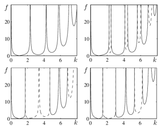
Figure 2: Examples of neutral stability curves $f(k)$ from (27) for various two-impulse forcing functions. Solid curves correspond to subharmonic tongues (Floquet multiplier $-1$), while dashed curves indicate harmonic tongues (Floquet multiplier $+1$). The spacing of the impulses, given by (17), is (a) $\Delta=0$, (b) $\Delta=0.05$, (c) $\Delta=\frac{1}{3}$, (d) $\Delta=\frac{1}{2}$. The dimensionless parameters in the calculations are $\gamma=0.02$ and $\Gamma_{0}=0.04$ (corresponding to fluid parameters $\nu=0.1$ ${\rm cm^{2}/s}$, $\Gamma=16$ dyn/cm, $\rho=1$ ${\rm g/cm}^{3}$, and $\frac{\omega}{2\pi}=20$ Hz).

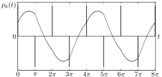
Figure 3: Eigenfunction $p_{k}(t)$ at $k=k_{c}$, $f=f_{c}$ for an impulsive forcing function with equally-spaced impulses. The dimensionless parameters used are $\gamma=0.17$, $\Gamma_{0}=0.19$ (roughly corresponding to physical parameters $\nu=0.20$ ${\rm cm^{2}/s}$, $\Gamma=16$ dyn/cm, $\rho=1$ ${\rm g/cm}^{3}$, and $\frac{\omega}{2\pi}=80$ H). Note the discontinuities in the derivative of $p_{k}(t)$ induced by the impulses at $t=n\pi$.

The expression for the neutral stability curve $f(k)$, given by (27), diverges at each value of $k$ for which $\cos(2\pi\omega_{k})=\cos(2\pi\omega_{k}\Delta)$. This leads to the structure of clearly demarcated resonance tongues seen in Fig. 2. The presence of vertical boundaries between resonance tongues contrasts sharply with the classical case of sinusoidal forcing (Fig. 4(a)), where multiple instabilities (involving distinct tongues) can occur for a single wavenumber. We now examine in more detail the spacing and sequence of resonant tongues in the case of two impulses per period. It proves useful, for the purposes of this analysis, to use $\omega_{k}$ as the independent variable, where $\omega_{k}$ and $k$ are related through the monotonic dispersion relation (11).

The divergence of the neutral curves, which leads to vertical asymptotes separating the resonance tongues, is due to the denominator in expression (27). We therefore introduce

$$D(\omega_{k})\equiv\cos(2\pi\omega_{k})-\cos(2\pi\omega_{k}\Delta),$$ (28)

and denote the successive zeroes of $D(\omega_{k})$ by $\omega_{k}^{j}$ ($\omega_{k}^{j}<\omega_{k}^{j+1}$, $\omega_{k}^{0}=0$). Since for $k>0$ the numerator of the expression inside the square root in (27) is strictly positive in the harmonic case and negative in the subharmonic case, it follows that $D(\omega_{k})>0$ for harmonic resonance tongues and $D(\omega_{k})<0$ for subharmonic resonance tongues.

In the general case, resonance tongues will alternate between harmonic and subharmonic as $k$ (equivalently, $\omega_{k}$) increases and $D(\omega_{k})$ alternates in sign. However, for special values of $\Delta$, successive subharmonic (or harmonic) tongues may occur. Specifically, this happens for some $j$ if $D(\omega_{k}^{j})=D^{\prime}(\omega_{k}^{j})=0$. We denote these double zeroes by $\hat{\omega}_{k}^{m},\ m\in\mathbb{Z^{+}}$ ($\hat{\omega}_{k}^{m}<\hat{\omega}_{k}^{m+1}$). It is straightforward to show that these degenerate values occur only when $\cos(2\pi\hat{\omega}_{k}^{m})=\cos(2\pi\hat{\omega}_{k}^{m}\Delta)=\pm 1$, which implies $\Delta=\frac{p}{q}$ for some co-prime integers $p,q$ ($0\leq p<q$). There are thus two possibilities: either both $p$ and $q$ are odd, or one of them is even. If they are both odd, then $\hat{\omega}_{k}^{m}=\frac{m}{2}q$; successive subharmonic (harmonic) tongues occur when $m$ is even (odd). (See Fig. 2(c), generated with $\Delta=\frac{1}{3}$.) In contrast, if either $p$ or $q$ is even (or $p=0$), then only subharmonic tongues can occur in succession; these are separated by vertical asymptotes at $\hat{\omega}_{k}^{m}=mq$. (See Fig. 2(a) and (d) for examples of this case.) Note that when $\Delta=0$ there are vertical asymptotes at each integer value of $\omega_{k}$ separating successive subharmonic tongues. In other words, there are no harmonic resonance tongues for equally-spaced impulses (Fig. 2(a)), as previously noted by Bechhoefer and Johnson Bechhoefer and Johnson (1996).

The maximum possible width for the resonance tongues occurs when $\Delta=0$, in which case $\omega_{k}^{j+1}-\omega_{k}^{j}=1$. As $\Delta$ is perturbed away from $0$, the vertical asymptotes (located at $\omega_{k}^{j}=\hat{\omega}_{k}^{j}=j$ for $\Delta=0$) split, and a thin harmonic tongue appears between them thereby separating the two fat subharmonic tongues (see, for example, Fig. 2(b)). Analogous results hold when $\Delta$ is perturbed away from other rational numbers.

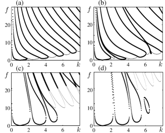
Figure 4: Neutral stability curves for truncated Fourier series approximations of equally spaced impulses with (a) 1 term, (b) 2 terms, (c) 10 terms, and (d) 20 terms. Large points correspond to subharmonic tongues and the smaller points to harmonic tongues. Parameters are the same as those in Fig. 2. Curves were generated using the method described in Kumar and Tuckerman (1994); Besson et al. (1996).

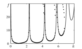
Figure 5: Neutral stability curve for impulsive forcing with $\Delta=0$ (solid lines) and a truncated Fourier series approximation with 50 terms (dots). Note that the 5th (rightmost) resonance tongue is not captured at all by the approximation. Parameters are as in Fig. 2.

II.2.3 Comparison with sinusoidal and multifrequency forcing

We now compare the linear stability results for equally-spaced impulsive forcing (i.e., $\Delta=0$) with the corresponding results for sinusoidal forcing

$$G_{\sin}(t)=f_{\sin}\sin(t).$$ (29)

Here $f_{\sin}\equiv\frac{g_{\sin}k_{0}}{\omega^{2}}$, where $g_{\sin}$ is the maximum (dimensioned) acceleration. (See Fig. 4(a) for an example of a neutral curve in the case of sinusoidal forcing.) As noted earlier, the most striking difference between these two cases, manifest in the neutral stability curve (27), is the lack of harmonic tongues for the impulsive case. This difference is a consequence of how the Floquet multipliers move in the complex plane as the perturbation wavenumber $k$ is varied, as illustrated in Fig. 6. In both the sinusoidal and the impulsive cases, the Floquet multipliers at $k=0$ (labeled as point 1 in Figs. 6(a,b)) are degenerate and take the value $+1$. As $k$ is increased from $0$, these split into a complex conjugate pair lying inside the unit circle which, together, sweep out a path encircling the origin. When $k$ reaches a certain value the Floquet multipliers meet again on the negative real axis and, at this point (labeled 2), are degenerate. With additional increase in $k$, they separate and move in opposite directions along the (negative) real axis. If the magnitude of $f$ exceeds the critical value (as it does in Figs. 6(a,b)), then the most negative Floquet multiplier eventually crosses $-1$, indicating a subharmonic instability. In any case, as $k$ is increased further, these (real) Floquet multipliers soon reverse direction and recombine (point 3) before splitting into a complex conjugate pair that moves to the right, again encircling the origin, before merging on the positive real axis (point 4). It is here that the difference between the two cases emerges. With sinusoidal forcing the Floquet multipliers split and move along the real axis; a harmonic instability will therefore develop if the forcing is strong enough to drive the rightmost Floquet multiplier outside the unit circle. In contrast, the Floquet multipliers in the impulsive case do not split along the positive real axis but simply continue their trajectory around the origin as a complex conjugate pair.

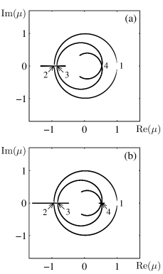
Figure 6: Floquet multipliers $\mu_{\pm}$ of Eq. (30) plotted in the complex plane over the range $k\in(0,3]$ with $f=f_{c}(1+1.4)$ (this forcing is well above the onset value for the first resonance tongue but below onset for the second) for (a) equally-spaced impulses, and (b) sinusoidal forcing. These cases differ in that only for sinusoidal forcing do the Floquet multipliers split on the positive real axis. Fluid parameters are as in Fig. 2. Numbers denote points described in the text.

The above description follows directly from an examination of the Floquet multipliers in (25):

$$\mu_{\pm}=e^{-2\pi\gamma k^{2}}\left(\alpha\pm\sqrt{\alpha^{2}-1}\right),$$ (30)

where, for $\Delta=0$,

$$\alpha\equiv{1\over 2}{\rm Tr}(M_{k})=\cos(2\pi\omega_{k})-\frac{1}{2}\left(\frac{fk\sin(\pi\omega_{k})}{\omega_{k}}\right)^{2}\leq 1.$$ (31)

From (30) we see that the Floquet multipliers are real and distinct whenever $\alpha^{2}>1$. However, since $\alpha\leq 1$, this can happen only when $\alpha<-1$, in which case they are negative.

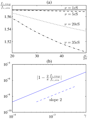
Figure 7: (a) Ratio of critical forcing strength for impulsive and sinusoidal forcing as a function of forcing frequency. Viscosities are labeled in the figure; other parameters are as in Fig. 2. The solid line for $\nu=1{\rm cS}$ is indistinguishable from a horizontal line at $\frac{\pi}{2}$. (b) Log-log plot of $|1-\frac{2}{\pi}\frac{f_{c,imp}}{f_{c,sin}}|$ as a function of $\gamma$ with $\Gamma_{0}=0.13$ (solid line). For comparison, a line of slope two is drawn nearby (dashed line).

To further compare equally-spaced impulses and sinusoidal forcing, we consider the respective critical forcing strengths at the onset of standing waves, $f_{c,imp}$ and $f_{c,sin}$. In the limit of weak damping we may expand (27) about $\gamma=0$ and $\omega_{k}=\frac{1}{2}$ (near the minimum of the neutral stability curves for small $\gamma$) to obtain

$$f_{c,imp}=\pi k_{c}\gamma(1+O(\gamma^{2})).$$ (32)

For sinusoidal forcing and small damping we have

$$f_{c,sin}=2k_{c}\gamma(1+O(\gamma^{2})),$$ (33)

(see, for example, Porter and Silber (2004)). Thus $\frac{f_{c,imp}}{f_{c,sin}}=\frac{\pi}{2}+O(\gamma^{2})$. This is the same ratio that arises when considering (the first term in) the Fourier series expansion of the two-term impulsive forcing function with $\Delta=0$:

$$G_{imp}(t)=\frac{2}{\pi}f_{imp}\sum_{j=0}^{\infty}\cos((2j+1)t).$$ (34)

Here we have used (5) and (18) with $f_{n}=(-1)^{n}f_{imp}$. In Fig. 7(a) we plot the ratio $\frac{f_{c,imp}}{f_{c,sin}}$ as a function of forcing frequency (the most easily tuned parameter in experiments) for several viscosities. As anticipated, for small $\nu$ this ratio is well approximated by $\frac{\pi}{2}$. Furthermore, the ratio decreases with increasing viscosity (equivalently, $\gamma$) with a deviation $|1-\frac{2f_{c,imp}}{\pi f_{c,sin}}|=O(\gamma^{2})$ (see Fig. 7(b)).

We may also consider the effect of adding a second term, $\cos(3t)$, to the truncation of the Fourier series (34) and examine $f_{c,2}$, the critical value of this two-frequency forcing function, in the weak damping limit. (In general, $f_{c,M}$ denotes the dimensionless forcing strength at onset for the $M$-term truncation of (34).) It is demonstrated in Topaz and Silber (2002) that for a two-frequency forcing function with commensurate frequencies $m\omega$ and $n\omega$ ($m\omega$ is assumed to drive the primary instability), the $n\omega$ frequency component is destabilizing when $\frac{m}{n}<\sqrt[4]{2}\approx 1.19$. By this we mean that the threshold for instability is lower in the two-frequency case than in the single frequency case. For the two-term truncation of (34), $\frac{m}{n}=\frac{1}{3}$ and hence we expect that $f_{c,2}<f_{c,1}=\frac{\pi}{2}f_{c,sin}$, i.e., $\frac{f_{c,2}}{f_{c,sin}}<\frac{\pi}{2}$. Indeed, this is consistent with our finding that $\frac{f_{c,imp}}{f_{c,sin}}<\frac{\pi}{2}$ for impulsive forcing (see Fig. 7(a)).

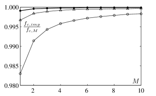
Figure 8: Ratio of critical forcing strengths for equally-spaced impulses and the $M$-term truncated Fourier series, as a function of $M$, for $\Gamma_{0}=0.04$ and $\gamma=0.02$ (filled circles), $\gamma=0.04$ (triangles), $\gamma=0.1$ (open circles).

As expected, adding more terms to the truncation of the Fourier series (34) results in a closer approximation to the critical forcing strength $f_{c,imp}$, as shown in Fig. 8. Despite this good agreement between $f_{c,imp}$ and $f_{c,M}$, the $M$-term truncated Fourier series is far less successful in capturing the behavior of the resonance tongues away from the minimum of the first tongue; this can be seen in Fig. 4. For $\gamma=0.02$ and $\Gamma_{0}=0.04$, for example, $f_{c,M}$ approximates $f_{c,imp}$ remarkably well even for small $M$ (filled circles in Fig. 8); however, with $M=50$, only the first four resonance tongues plausibly resemble those for impulsive forcing (see Fig. 5).

III Weakly nonlinear analysis

III.1 Weakly nonlinear calculation

We now extend our analysis of $N=2$ impulses to the weakly nonlinear regime in the case of one-dimensional waves.

Following Silber and Skeldon (1999), we perform a multi-scale expansion:

$$h(x,t,T) =\epsilon h_{1}(x,t,T)+\epsilon^{2}h_{2}(x,t,T)+\cdots,$$ (35a)

$$\Phi(x,t,T) =\epsilon\Phi_{1}(x,t,T)+\epsilon^{2}\Phi_{2}(x,t,T)+\cdots,$$ (35b)

where $\epsilon\ll 1$, the slow time is $T=\epsilon^{2}t$, and the forcing amplitude is $f=f_{c}(1+\epsilon^{2}f_{2})$. We seek spatially-periodic solutions in separable Floquet-Fourier form:

$$h_{1}(x,t,T) =Z(T)p_{1}(t)e^{ik_{c}x}+c.c.,$$ (36a)

$$h_{2}(x,t,T) =Z^{2}(T)p_{2}(t)e^{2ik_{c}x}+c.c.,$$ (36b)

$$\Phi_{1}(x,t,T) =Z(T)q_{1}(t)e^{ik_{c}x}+c.c.,$$ (36c)

$$\Phi_{2}(x,t,T) =Z^{2}(T)q_{2}(t)e^{2ik_{c}x}+c.c.,$$ (36d)

where the critical wave number $k_{c}$, and the periodic eigenfunction $p_{1}(t)$ are determined from the linear stability analysis. Specifically, we take $(k_{c},f_{c})$ to be the minimum of the neutral stability curves and use (10), evaluated at $k=k_{c}$ and with $|A_{k_{c},n}|=1$, to obtain $p_{1}(t)$. The phase of $A_{k_{c},n}$ is determined by the map (25), evaluated at $(k,f)=(k_{c},f_{c})$, and the (subharmonic) condition $p_{1}(t+2\pi)=-p_{1}(t)$ (equivalently, $A_{k_{c},n+2}=-A_{k_{c},n}$):

$$\frac{A_{k_{c},n}^{i}}{A_{k_{c},n}^{r}}=\frac{\cos(2\pi\omega_{k_{c}})-F_{n}c_{n}s_{n+1}+e^{2\pi\gamma k_{c}^{2}}}{\sin(2\pi\omega_{k_{c}})-F_{n}s_{n}s_{n+1}}.$$ (37)

This expression defines the critical eigenmode associated with the instability. The subharmonic assumption $A_{k_{c},n+2}=-A_{k_{c},n}$ is valid when the instability is associated with the first resonance tongue, as it is for all parameters we have investigated. Plugging (36c) into (1a) yields $q_{1}(t)=\frac{1}{k_{c}}(p_{1}^{\prime}(t)+\gamma k_{c}^{2}p_{1}(t))$ at leading order in $\epsilon$. Since in this section $k$ will generally be fixed at its critical value, we hereafter drop this subscript from many expressions (e.g., we write $A_{n}$ for $A_{k_{c},n}$) or replace it with a subscript 1 (such as with $p_{1}(t)$).

At second order we find the equation (cf. (9))

$$q_{1}^{2}= \ p_{2}^{\prime\prime}+2\gamma(2k_{c})^{2}p_{2}^{\prime}$$

$$+[\gamma^{2}(2k_{c})^{4}+\Gamma_{0}(2k_{c})^{3}+(G_{0}-G(t))2k_{c}]p_{2},$$ (38)

which has the solution

$$p_{2}(t)= \ aA_{n}^{2}e^{2(-\gamma k_{c}^{2}+i\omega_{1})(t-t_{n})}+\frac{1}{2}b|A_{n}|^{2}e^{-2\gamma k_{c}^{2}(t-t_{n})}$$

$$+B_{n}e^{(-\gamma(2k_{c})^{2}+i\omega_{2})(t-t_{n})}+c.c.,$$ (39)

for $t\in(t_{n},t_{n+1})$. Here

$$a=\frac{-2k_{c}\omega_{1}^{2}}{\omega_{2}^{2}-4\omega_{1}^{2}+4\gamma^{2}k_{c}^{2}+8i\gamma k^{2}\omega_{1}},$$ (40)

$$b=\frac{4k_{c}\omega_{1}^{2}}{\omega_{2}^{2}+4\gamma^{2}k_{c}^{4}},$$ (41)

and $\omega_{1}\ (\omega_{2})$ is the frequency of a wave with wavenumber $k_{c}\ (2k_{c})$ obtained from the dispersion relation (4). Note that the “homogeneous” solution to (38) must be included (i.e., $B_{n}\neq 0$) to ensure that $p_{2}(t)$ is continuous. Using this continuity condition and the jump condition on $p^{\prime}_{2}$ (obtained as in the linear stability calculation), we relate $B_{n+1}$ to $B_{n}$ through the map

$$\left(\begin{array}[]{c}B_{n+1}^{r}\\ B_{n+1}^{i}\end{array}\right)=e^{-4\gamma k_{c}^{2}d_{n}}M_{2,n}\left(\begin{array}[]{c}B_{n}^{r}\\ B_{n}^{i}\end{array}\right)+R_{n}+bS_{n}.$$ (42)

Here $M_{2,n}$ is the matrix $M_{k,n}$ of (14) with $k=2k_{c}$; the vectors $R_{n}$ and $S_{n}$ are given in the Appendix. To obtain $B_{n}$, we require that $B_{n+2}=B_{n}$. (This harmonic condition is due to the fact that $q_{1}^{2}$, the driving term in (38), is $2\pi$-periodic.)

At third order we obtain the solvability condition (see Silber and Skeldon (1999))

$$\tau\frac{dZ}{dT}=Lf_{2}Z+(C_{res}+C_{non})|Z|^{2}Z,$$ (43)

where $\tau$, $L$, $C_{res}$ and $C_{non}$ are given by

$$\tau =\frac{1}{2\pi}\int_{0^{-}}^{4\pi^{-}}(p_{1}^{\prime}+\gamma k_{c}^{2}p_{1})\tilde{p}_{1}dt$$ (44a)

$$=\frac{1}{2\pi}(A_{0}\tilde{A_{0}}(e^{i\omega_{1}d_{0}}-1-i\omega_{1})$$

$$\ \ \ \ \ \ +A_{1}\tilde{A_{1}}(e^{i\omega_{1}d_{1}}-1-i\omega_{1}))+c.c.,$$

$$L =\frac{k_{c}}{4\pi}\int_{0^{-}}^{4\pi^{-}}{G_{imp}(t)\over f}p_{1}\tilde{p}_{1}dt$$ (44b)

$$=\frac{k_{c}}{2\pi}(A_{0}\tilde{A_{0}}+A_{0}\overline{\tilde{A}}_{0}-A_{1}\tilde{A_{1}}-A_{1}\overline{\tilde{A}}_{1})+c.c.,$$

$$C_{res} =-\frac{k_{c}^{2}}{2\pi}\int_{0^{-}}^{4\pi^{-}}[(q_{1}p_{2})^{\prime}+\gamma k_{c}^{2}q_{1}p_{2}]\tilde{p}_{1}dt,$$ (44c)

$$C_{non} =\frac{k_{c}^{3}}{4\pi}\int_{0^{-}}^{4\pi^{-}}[-(p_{1}^{2}q_{1})^{\prime}-\gamma k_{c}^{2}p_{1}^{2}q_{1}+k_{c}q_{1}^{2}p_{1}$$ (44d)

$$\ \ \ \ \ \ +\frac{3}{2}k_{c}^{2}\Gamma_{0}p_{1}^{3}]\tilde{p}_{1}dt.$$

The full expressions for $C_{res}$ and $C_{non}$ are provided in the Appendix. In equations (44) we use $\tilde{p}_{1}$ to indicate the solution of the adjoint linear problem, which has the same form as (8) but with $\gamma\rightarrow-\gamma$. Hence

$$\tilde{p}_{1}(t)=\tilde{A}_{n}e^{(\gamma k^{2}+i\omega_{1})(t-t_{n})}+c.c.,\quad t\in(t_{n},t_{n+1})\ ,$$ (45)

with the complex conjugate of $\tilde{A}_{n}$ denoted by $\overline{\tilde{A}}_{n}$. The map relating $\tilde{A}_{n+1}$ to $\tilde{A}_{n}$ is similarly obtained from (13) by replacing $\gamma$ with $-\gamma$ and setting $k=k_{c}$. Note that in (43) we separate the cubic coefficient $C$ into two distinct contributions, $C_{res}$ (resonant) and $C_{non}$ (nonresonant). The $C_{res}$ term can be traced to quadratic nonlinearities in (1) (i.e., terms in which the $k_{c}$ and $2k_{c}$ modes interact), while $C_{non}$ derives from cubic nonlinearities and involves only the critical $k_{c}$ mode.

III.2 Weakly nonlinear results

We now examine in greater detail the cubic coefficient $C=C_{res}+C_{non}$, which determines the nonlinear saturation of the instability to standing waves. Figs. 9(a,b) show $C$ as a function of the capillary parameter $\Gamma_{0}$ for various choices of $\Delta$. We find, for most parameters, that $C(\Gamma_{0})<0$, ensuring that the bifurcation to standing waves is supercritical. (We find subcritical bifurcations only in the capillary wave regime, $\Gamma_{0}\approx 0.25$, and with extreme asymmetry, e.g. $\Delta\approx 0.99$.)

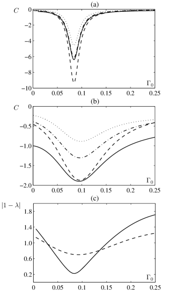
Figure 9: Cubic coefficient in (43) as a function of $\Gamma_{0}$ with (a) $\gamma=0.01$ and (b) $\gamma=0.05$. The dashed line indicates the result for impulsive forcing with $\Delta=0.5$; the dot-dashed line is for $\Delta=0$; the dotted is for $\Delta=-0.5$; the solid line is for sinusoidal forcing. (c) $|1-\lambda|$ as a function of $\Gamma_{0}$ where $\lambda$ and $\overline{\lambda}$ are the Floquet multipliers (30) of the $2k_{c}$ mode for $\Delta=0$ and $\gamma=0.01$ (solid line) or $\gamma=0.05$ (dashed line).

A dominant feature of the curves shown in Figs. 9(a,b) is the dip in $C$ that reaches a minimum value at $\Gamma_{0}=\Gamma_{res}\sim 0.09$. This resonance feature is apparent both with impulsive forcing (non-solid lines in Figs. 9(a,b)) and with sinusoidal forcing (solid lines). For this figure we have used a normalization convention for $p_{1}(t)$ in the sinusoidal case which agrees with our normalization convention in the impulsive case ($|A_{k_{c},n}|=1$) in the limit $\gamma\to 0$. Note that the sinusoidal and impulsive results agree quantitatively for $\gamma=0.01$ and $\Delta=0$. For larger damping ($\gamma=0.05$), the sinusoidal curve is shifted relative to the impulsive ones indicating a difference between their nonresonant contributions $C_{non}$ to $C$.

In the sinusoidal case, the dip in $C$ is easily attributed to a 1:2 spatio-temporal resonance, i.e., at $\Gamma_{res}$ we have $2\omega_{1}=\omega_{2}$ (see Zhang and Viñals (1997), for example). The strength of this feature, which scales with $1/\gamma$, is due to the strong coupling between the first subharmonic and the first harmonic modes, which become spatially commensurate at $\Gamma_{res}$. Since harmonic resonance tongues are entirely absent from the neutral stability picture for equally-spaced impulses, it is perhaps surprising that the dip appears in this case as well. However, we can understand its origin in the following way (see Silber and Skeldon (1999) for an analogous argument in the case of two-frequency forced Faraday waves). We express the height of spatially-periodic surface waves at integer multiples of the forcing period in the form

$$h(x,t_{m})=z_{m,\mu}e^{ik_{c}x}+w_{m,\lambda}e^{i2k_{c}x}+v_{m,\overline{\lambda}}e^{i2k_{c}x}+\cdots+c.c.,$$ (46)

where $t_{m}=2\pi m$, $m\in\mathbb{Z}$. Here $\mu$ is the (real) Floquet multiplier of the $k_{c}$ mode while $\lambda$ and $\overline{\lambda}$ are the Floquet multipliers of the $2k_{c}$ mode(s), assumed to be complex. From the linear stability analysis, we know that the critical standing waves are subharmonic, i.e., at onset $\mu=-1$. Considering the symmetries of the problem, including spatial translation and reflection, we arrive at a stroboscopic map from the $m^{th}$ to $(m+1)^{st}$ period:

$$z_{m+1} = -z_{m}+(q_{1}w_{m}+\overline{q}_{1}v_{m})\overline{z}_{m}+a_{1}|z_{m}|^{2}z_{m}+\cdots,$$

$$w_{m+1} = \lambda w_{m}+q_{2}z_{m}^{2}+\cdots,$$ (47)

$$v_{m+1} = \overline{\lambda}v_{m}+\overline{q}_{2}z_{m}^{2}+\cdots,$$

where we have kept the terms that contribute at leading order to the cubic coefficient in (43). Because $w_{m}$ and $v_{m}$ are damped modes ($|\lambda|<1$), we may perform a center manifold reduction to eliminate them. This gives, at leading order,

$$w_{m}=-\frac{q_{2}}{(1-\lambda)}z_{m}^{2},\quad v_{m}=-\frac{\overline{q}_{2}}{(1-\overline{\lambda})}z_{m}^{2},$$ (48)

resulting in the map

$$z_{m+1}=-z_{m}+\left(a_{1}-\frac{q_{1}q_{2}}{(1-\lambda)}-\frac{\overline{q}_{1}\overline{q}_{2}}{(1-\overline{\lambda})}\right)|z_{m}|^{2}z_{m}.$$ (49)

If $\lambda$ and $\overline{\lambda}$ are close enough to one, then the slaved modes can make a large contribution to the cubic coefficient $C$. Using the Floquet analysis of Section II.2, we confirm that for $\Gamma_{0}=\Gamma_{res}$ the Floquet multipliers associated with the $2k_{c}$ mode come closest to one, i.e., at that point the Floquet multipliers cross the positive real axis (see Fig. 9(c)). This resonant contribution to the cubic coefficient $C$ becomes increasingly pronounced as the damping decreases (compare the vertical scales in Figs. 9(a) and (b)).

A comparison of the (non-solid) curves in Figs. 9(a,b) reveals that the spacing of the impulses can have a significant effect on the magnitude of the resonance feature. Some explanation for this behavior is provided by recent results Porter et al. (2004); Topaz et al. (2004) on multifrequency forced Faraday waves in which the form of the cubic amplitude equations is obtained from the spatial symmetries and the (weakly broken) symmetries of time translation, time reversal, and Hamiltonian structure. Such a procedure yields important qualitative features of the behavior of the critical modes and other damped modes driven through nonlinear interactions, including a prediction about which particular damped modes are most important and which forcing frequencies (and corresponding temporal phases) are most effective in enhancing or otherwise controlling their effect. Here we are interested in the Fourier series expansion for an impulsive forcing function with two impulses per period:

$$G_{imp}(t)=\frac{f_{imp}}{2\pi}\sum_{j=1}^{\infty}(1-e^{-ij((1+\Delta)\pi)})e^{ijt}+c.c.$$ (50)

In Porter et al. (2004); Topaz et al. (2004) the contribution of the damped $2k_{c}$ mode to the 1:2 spatio-temporal resonance is found to be most affected by the forcing frequency $2\omega$ (where $\omega$ is the primary driving frequency) and its phase. This result suggests that we focus on the drastically truncated two-term Fourier series

$$G_{2}(t)=\frac{f_{imp}}{2\pi}\left[(1+e^{-i\pi\Delta})e^{it}+(1-e^{-2i\pi\Delta})e^{2it}+c.c.\right].$$ (51)

At leading order in the damping $\gamma$, the onset of standing waves occurs when the magnitude of the first term in (51) becomes equal to $\gamma$ (see, for example, Porter and Silber (2004)). Using

$$\frac{f_{imp}}{2\pi}|1+e^{-i\pi\Delta}|=\gamma,$$ (52)

and simplifying the result through an appropriate time translation, we may rewrite (51) at onset as

$$G_{2}(t)=\gamma e^{it}+F_{2}e^{2it}+c.c.,$$ (53)

where

$$F_{2}=2i\gamma\sin\big{(}\Delta\frac{\pi}{2}\big{)}.$$ (54)

From Table 1 in Porter et al. (2004) we find the predicted magnitude, at leading order in $\gamma$, of the resonant dip in the cubic coefficient at $\Gamma_{res}$,

$$C_{res}^{2f}=-\alpha_{1}\frac{|L_{3}|+\mu_{i}|f_{2\Omega}|\sin\Phi}{|L_{3}|^{2}-|\mu_{i}f_{2\Omega}|^{2}},$$ (55)

Here $|f_{2\Omega}|=|F_{2}|=2\gamma\sin\left(\Delta\frac{\pi}{2}\right)$, $\Phi=\arg(F_{2})={\rm sign}(\Delta)\frac{\pi}{2}$, $L_{3}$ is the linear damping coefficient of the $2k_{c}$ mode ($L_{3}=(2k_{c})^{2}\gamma\approx 4\gamma$), and $\mu_{i}$ is the coefficient of the linear parametric driving term for the $2k_{c}$ mode ($\mu_{i}=\frac{2k_{c}}{2}\approx 1$). Thus $C_{res}^{2f}$, as a function of the asymmetry parameter $\Delta$, becomes

$$C_{res}^{2f}(\Delta)\approx-\frac{\alpha_{1}}{2\gamma}\ \frac{1}{2-\sin\left(\frac{\Delta\pi}{2}\right)}\,.$$ (56)

The constant $\alpha_{1}$ is positive and must be determined by a nonlinear calculation; it depends on $\Gamma_{0}$, but not, at leading order, on $\gamma$. Here we choose $\alpha_{1}$ such that the values of the multifrequency prediction $C_{res}^{2f}(\Delta)$ and our direct calculation of $C_{res}(\Delta)$ at $\Gamma_{0}=\Gamma_{res}$ from (A) agree for small damping ($\gamma=0.001$) at $\Delta=0$. (We then use the same estimate of $\alpha_{1}$ throughout this comparison.) We compare $C_{res}(\Delta)$ with the multifrequency prediction in Fig. 10 and find good agreement, especially for small $\gamma$ where the multifrequency results are expected to be valid. This agreement breaks down as $|\Delta|$ approaches unity (even more so for larger $\gamma$), an effect that is not overly surprising given that $|\Delta|\to 1$ is an unphysical limit requiring an infinite value of $f_{imp}$ to produce standing waves. Note that $C_{res}^{2f}$, given by (56), scales with $\gamma^{-1}$, which explains the difference in scales evident in Fig. 9(a,b).

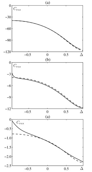
Figure 10: Resonant contribution $C_{res}$ to the cubic coefficient of Eq. (43) as a function of the asymmetry parameter $\Delta$ over the range $[-0.95,0.95]$, calculated for the Zhang-Viñals equations using (A) (solid line) and using multifrequency forcing results (56) with $\alpha_{1}=0.235$ (dashed line). Plots are for (a) $\gamma=0.001$, (b) $\gamma=0.01$, and (c) $\gamma=0.05$.

IV Discussion and Conclusions

In this paper we examined the problem of Faraday waves parametrically excited by a periodic sequence of impulses (delta functions). We showed how to extend the linear stability analysis presented in Bechhoefer and Johnson (1996) to include more general impulsive forcing functions, and investigated the weakly nonlinear regime for one-dimensional surface waves in the case of two impulses per period, comparing both linear and nonlinear results with the more established cases of sinusoidal and multifrequency forcing. Our analytical and numerical work was conducted within the framework of the Zhang-Viñals Faraday wave model, appropriate for describing small amplitude surface waves on deep, weakly-viscous fluid layers.

One theoretical advantage of using an idealized impulsive forcing function is that it allows for an exact, albeit generally implicit, expression for the neutral stability curves associated with the primary instability. Moreover, since the stroboscopic map characterizing the linear problem can be explicitly constructed, Floquet multipliers can be readily determined as a function of forcing and fluid parameters. This stands in sharp contrast to the sinusoidal and multifrequency cases where even the neutral curves must be determined numerically or through an asymptotic expansion that assumes weak damping and forcing. A further consequence of exactly solving the linear problem is that we are then able to derive explicit, analytic expressions for the amplitude of weakly nonlinear, one-dimensional surface waves as a function of forcing and fluid parameters.

As noted by Bechhoefer and Johnson (1996), in the simplest case of $N=2$ impulses per period, harmonic instabilities from the flat fluid state cannot be excited with equally-spaced impulses. Despite this fact, we found, through a weakly nonlinear analysis, that the 1:2 spatio-temporal resonance remains the dominant feature in typical parameter regimes. Symmetry arguments of the type used in Silber and Skeldon (1999) showed that, as in the case of sinusoidal forcing, harmonic modes can be driven nonlinearly by the critical modes — hence the resonance effect persists.

By varying the spacing between the up and down impulses making up the $2\pi$-periodic forcing function for $N=2$, we found that the magnitude of the 1:2 resonance effect depends dramatically, and monotonically, on the corresponding asymmetry parameter $\Delta$. Appealing to recent results from multifrequency forcing theory Topaz et al. (2004), valid in the limit of weak damping, we obtained a prediction of this dependence based on a truncated two-term Fourier series approximation. This prediction agreed quite well with the results for impulsive forcing despite the severity of the approximation involved.

We envision several ways in which this work could be extended. For example, the methods used in this paper could be easily applied to the case of piecewise constant forcing, a type of driving function that has been explored in other systems (see Hsu and Cheng (1973); Yorke (1978), for instance) where it also led to analytic results. It would further be of interest to extend our weakly nonlinear analysis to the case of two-dimensional patterns. In such a context, additional questions of pattern selection, as well as more specific comparisons with multifrequency forcing, could be explored. One could try, for example, to construct impulsive forcing functions that mimic specific effects seen with multifrequency forcing. In this way the analytic results available for impulsive forcing would complement the numerical Beyer and Friedrich (1995); Besson et al. (1996); Topaz and Silber (2002) and experimental results Edwards and Fauve (1993); Müller (1993); Edwards and Fauve (1994); Kudrolli et al. (1998); Arbell and Fineberg (1998, 2000a, 2002); Epstein and Fineberg (2004) reported with multifrequency forcing.

Appendix A Analytic Expressions

The vectors given in (42) are

$$R_{n}=\left(\begin{array}[]{c}Re[a(A_{n}^{2}e^{(-\gamma k_{c}^{2}+i\omega_{1})2d_{n}}-A_{n+1}^{2})]\\ \frac{2}{\omega_{2}}Re[a(A_{n}^{2}(e^{(-\gamma k_{c}^{2}+i\omega_{1})2d_{n}}((-1)^{n}k_{c}f_{c}-\gamma k_{c}^{2}-i\omega_{1})+A_{n+1}^{2}(\gamma k_{c}^{2}+i\omega_{1})))]\end{array}\right),$$ (57)

and

$$S_{n}=\left(\begin{array}[]{c}\frac{1}{2}(|A_{n}|^{2}e^{-2\gamma k_{c}^{2}d_{n}}-|A_{n+1}|^{2})\\ \frac{1}{\omega_{2}}(|A_{n}|^{2}e^{-2\gamma k_{c}^{2}d_{n}}((-1)^{n}2k_{c}f_{c}-\gamma k_{c}^{2})+|A_{n+1}|^{2}\gamma k_{c}^{2})\end{array}\right).$$ (58)

The expressions for $a$ and $b$ in these vectors are given by (40) and (41), respectively, and $\omega_{1}$ ($\omega_{2}$) satisfies the dispersion relation (4) with wavenumber $k_{c}$ ($2k_{c}$).

The full expressions for the components ($C_{res}$ and $C_{non}$) of the cubic coefficient in the solvability condition (43) are

$$C_{res} = \frac{-2i\omega_{1}k_{c}}{\pi}\sum_{j=0,1}A_{j}B_{j}\tilde{A_{j}}\frac{\beta_{1}^{+}-i\omega_{1}}{\beta_{1}^{+}}(e^{\beta_{1}^{+}d_{j}}-1)-\bar{A_{j}}B_{j}\bar{\tilde{A_{j}}}\frac{\beta_{1}^{-}+i\omega_{1}}{\beta_{1}^{-}}(e^{\beta_{1}^{-}d_{j}}-1)$$

$$+\left(A_{j}B_{j}\bar{\tilde{A_{j}}}\frac{\beta_{2}+i\omega_{1}}{\beta_{2}}-\bar{A_{j}}B_{j}\tilde{A_{j}}\frac{\beta_{2}-i\omega_{1}}{\beta_{2}}\right)(e^{\beta_{2}d_{j}}-1)$$

$$+\left(aA_{j}^{3}\bar{\tilde{A_{j}}}\frac{\beta_{3}+i\omega_{1}}{\beta_{3}}+(b-a)|A_{j}|^{2}A_{j}\tilde{A_{j}}\frac{\beta_{3}-i\omega_{1}}{\beta_{3}}\right)(e^{\beta_{3}d_{j}}-1)$$

$$+aA_{j}^{3}\tilde{A_{j}}\frac{\beta_{4}-i\omega_{1}}{\beta_{4}}(e^{\beta_{4}d_{j}}-1)+(b-a)|A_{j}|^{2}A_{j}\bar{\tilde{A_{j}}}\frac{2\gamma k_{c}^{2}-i\omega_{1}}{2\gamma k_{c}^{2}}(e^{-2\gamma k_{c}^{2}d_{j}}-1)+c.c.,$$

$$C_{non} = \sum_{j=0,1}\left(A_{j}^{3}\bar{\tilde{A_{j}}}+|A_{j}|^{2}A_{j}\tilde{A_{j}}\right)\frac{3\Gamma_{0}k_{c}^{5}-i\omega_{1}k_{c}^{2}\beta_{3}}{\pi\beta_{3}}(e^{\beta_{3}d_{j}}-1)$$

$$+A_{j}^{3}\tilde{A_{j}}\frac{3\Gamma_{0}k_{c}^{5}-2i\omega_{1}k_{c}^{2}\beta_{4}}{4\pi\beta_{4}}(e^{\beta_{4}d_{j}}-1)+|A_{j}|^{2}A_{j}\bar{\tilde{A_{j}}}\frac{4i\gamma\omega_{1}k_{c}^{4}-9\Gamma_{0}k_{c}^{5}}{8\pi\gamma k_{c}^{2}}(e^{-2\gamma k_{c}^{2}d_{j}}-1)+c.c.,$$

where

$$\beta_{1}^{\pm}=-4\gamma k_{c}^{2}+i(\pm 2\omega_{1}+\omega_{2}),\ \beta_{2}=-4\gamma k_{c}^{2}+i\omega_{2},\ \beta_{3}=-2\gamma k_{c}^{2}+2i\omega_{1},\ \beta_{4}=-2\gamma k_{c}^{2}+4i\omega_{1}.$$ (61)

References

- Zhang and Viñals (1997) W. Zhang and J. Viñals, J. Fluid Mech. 336, 301 (1997).
- Bechhoefer and Johnson (1996) J. Bechhoefer and B. Johnson, Am. J. Phys. 64, 1482 (1996).
- Porter et al. (2004) J. Porter, C. M. Topaz, and M. Silber, Phys. Rev. Lett. 93 (2004).
- Topaz et al. (2004) C. M. Topaz, J. Porter, and M. Silber, Phys. Rev. E 70, 066206 (2004).
- Faraday (1831) M. Faraday, Phil. Trans. R. Soc. Lond. 121, 319 (1831).
- Miles and Henderson (1990) J. Miles and D. Henderson, Ann. Rev. Fluid Mech. 22, 143 (1990).
- Müller et al. (Springer, 1998) H. W. Müller, R. Friedrich, and D. Papathanassiou, in Evolution of Spontaneous Structures in Dissipative Continuous Systems, edited by F. H. Busse and S. C. Muller Lecture Notes in Physics pp. 231–265 (Springer, 1998).
- Christiansen et al. (1992) B. Christiansen, P. Alstrom, and M. T. Levinsen, Phys. Rev. Lett. 68, 2157 (1992).
- Kudrolli and Gollub (1996) A. Kudrolli and J. P. Gollub, Physica D 97, 133 (1996).
- Binks and van der Water (1997) D. Binks and W. van der Water, Phys. Rev. Lett. 78, 4043 (1997).
- Wagner et al. (2000) C. Wagner, H. W. Müller, and K. Knorr, Phys. Rev. E 62, R33 (2000).
- Edwards and Fauve (1994) W. S. Edwards and S. Fauve, J. Fluid Mech. 278, 123 (1994).
- Kudrolli et al. (1998) A. Kudrolli, B. Pier, and J. P. Gollub, Physica D 123, 99 (1998).
- Arbell and Fineberg (1998) H. Arbell and J. Fineberg, Phys. Rev. Lett. 81, 4384 (1998).
- Edwards and Fauve (1993) W. S. Edwards and S. Fauve, Phys. Rev. E 47, R788 (1993).
- Arbell and Fineberg (2000a) H. Arbell and J. Fineberg, Phys. Rev. Lett. 84, 654 (2000a).
- Müller (1993) H. W. Müller, Phys. Rev. Lett. 71, 3287 (1993).
- Arbell and Fineberg (2000b) H. Arbell and J. Fineberg, Phys. Rev. Lett. 85, 756 (2000b).
- Arbell and Fineberg (2002) H. Arbell and J. Fineberg, Phys. Rev. E 65, 036224 (2002).
- Epstein and Fineberg (2004) T. Epstein and J. Fineberg, Phys. Rev. Lett. 92, 244502 (2004).
- Benjamin and Ursell (1954) T. B. Benjamin and F. Ursell, Proc. Roy. Soc. Lond. Ser. A 225, 505 (1954).
- Kumar and Tuckerman (1994) K. Kumar and L. S. Tuckerman, J. Fluid Mech. 279, 49 (1994).
- Beyer and Friedrich (1995) J. Beyer and R. Friedrich, Phys. Rev. E 51, 1162 (1995).
- Kumar (1996) K. Kumar, Proc. Roy. Soc. Lond. A 452, 1113 (1996).
- Chen and Viñals (1997) P. Chen and J. Viñals, Phys. Rev. Lett. 79, 2670 (1997).
- Besson et al. (1996) T. Besson, W. S. Edwards, and L. S. Tuckerman, Phys. Rev. E 54, 507 (1996).
- Chen and Viñals (1999) P. Chen and J. Viñals, Phys. Rev. E 60, 559 (1999).
- Golubitsky et al. (1988) M. Golubitsky, I. Stewart, and D. Schaeffer, Singularities and Groups in Bifurcation Theory: Vol. II, no. 69 in Appl. Math. Sci. Ser (Springer–Verlag, New York, 1988).
- Crawford and Knobloch (1991) J. D. Crawford and E. Knobloch, Annu. Rev. Fluid Mech. 23, 341 (1991).
- Silber and Proctor (1998) M. Silber and M. R. E. Proctor, Phys. Rev. Lett. 81, 2450 (1998).
- Tse et al. (2000) D. P. Tse, A. M. Rucklidge, R. B. Hoyle, and M. Silber, Physica D 146, 367 (2000).
- Silber and Skeldon (1999) M. Silber and A. Skeldon, Phys. Rev. E 59, 5446 (1999).
- Topaz and Silber (2002) C. M. Topaz and M. Silber, Physica D 172, 1 (2002).
- Porter and Silber (2004) J. Porter and M. Silber, Physica D 190, 93 (2004).
- Hsu (1972) C. S. Hsu, J. Appl. Mech. 39, 551 (1972).
- Hsu and Cheng (1973) C. S. Hsu and W. H. Cheng, J Appl. Mech. E40, 78 (1973).
- Pilipchuk et al. (1999) V. N. Pilipchuk, S. A. Volkova, and G. A. Starushenko, J. Sound and Vibration 222, 307 (1999).
- Huepe and Silber (in prep.) C. Huepe and M. Silber (in prep.).
- Yorke (1978) E. D. Yorke, Am. J. Phys. 46, 285 (1978).