Experimental Synchronization of Spatiotemporal Chaos
in Nonlinear Optics

Abstract

We demonstrate that a unidirectional coupling between a pattern forming system and its replica induces complete synchronization of the slave to the master system onto a spatiotemporal chaotic state.

In recent years, synchronization of complex systems have attracted a great interest in the scientific community synchro , as well as in the literature oriented to lay audiences stro03 . This indicates the behavior of two (or many) systems (either equivalent or non equivalent) that adjust a common feature of their complex dynamics due to a coupling or to a forcing.

For time chaotic systems, four types of synchronization have mostly been studied, namely complete synchronization (CS), phase (PS) and lag (LS) synchronization, and generalized synchronization (GS). CS refers to a process whereby two interacting systems perfectly link their chaotic trajectories, thus remaining in step with each other in the course of the time complete . GS implies the hooking of the output of one system to a given function of the output of the other system rul . PS is characterized by a locking of the phases of the two signals, also in the absence of a substantial correlation between the two chaotic amplitudes phase . Finally, LS consists in the hooking of one system to the lagged output of the other intermittentlag . All these effects have been explored in natural phenomena nature , and laboratory experiments exp , and unified approaches to describe def and measure synchronization states have been proposed.

When the interest shifted to space-extended systems, synchronization phenomena were shown in large populations of coupled chaotic units and neural networks pop , globally or locally coupled map lattices map , and pattern forming systems governed by partial differential equations stc . Here, however, all theoretical and numerical progresses were accompanied by a substantial lack of experimental verifications. Precisely, CS of spatiotemporal patterns was first observed in chemistry chemistry for two mutually coupled Belouzov-Zhabotinski cells, where, however, the resulting synchronized state corresponded to the suppression of spatiotemporal complexity and the emergence of a common spiral behavior. Later on, LS was observed in a pair of unidirectionally coupled nonlinear optical systems neubecker . The evidence here was given in terms of an improvement in the lagged correlation between the master and slave patterns. Finally, GS was demonstrated in an open loop liquid crystal light modulator with optoelectronic feedback roy by the use of the so called auxiliary system method rul .

In this Letter we report the first direct experimental evidence of complete synchronization on unidirectionally coupled pattern forming systems. At variance with what observed in Ref. chemistry , the resulting synchronized state here corresponds to a spatiotemporal chaotic dynamics where the slave system is identically attained to the behavior of the master system.

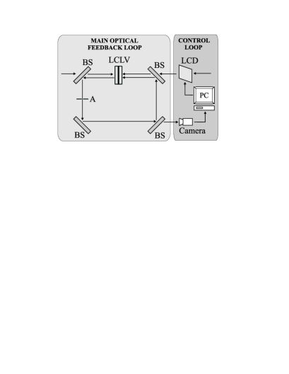
Figure 1: a) Experimental setup. Main loop: an expanded laser beam is closed through a non-linear Kerr-like medium (liquid crystal optical valve). BS: beam splitters; A: aperture in a Fourier plane. Control arm: PC: personal computer; LCD: liquid crystal display.

The experimental setup is sketched in Fig. 1. A main optical feedback loop (MOFL) consists of a Liquid Crystal Light Valve (LCLV) with optical feedback AkhmanovNoiChaos . The LCLV induces on the reading light a phase delay proportional to the writing intensity (Kerr-like effect). This proportionality relation holds for all experimental parameters used in the present investigation. The pattern forming mechanism acts on an homogeneous pump wave of intensity $I_{p}$ sent onto the front face of the LCLV. The wave is totally reflected and acquires a spatial phase modulation. Diffractive propagation along the MOFL provides conversion of phase into amplitude modulations. Due to the Kerr-like behaviour of the LCLV, these amplitude modulations are converted back to phase modulations, so that eventually a positive feedback establishes for some spatial frequencies, which are destabilized resulting in pattern formation.

An additional electro-optic control loop is constituted by a video-camera and a personal computer driving a liquid crystal display (LCD). The control signal is a laser beam that traverses the LCD before being injected into the MOFL. The LCD display is operating in transmission, and encodes linearly the gray level images output by the PC, onto the laser beam traversing it.

When the control loop is open, the dynamics of the optical beam phase $\phi(x,y,t)$ at the LCLV output can be described by Firth ; NeubeckerOppo $\frac{\partial\phi}{\partial t}=-\frac{1}{\tau}(\phi-\phi_{0})+D\nabla^{2}\phi+\alpha I_{fb}$, where $\phi_{0}$ is the working reference phase, $\tau$ the LCLV relaxation time, $D$ a diffusion coefficient, $\alpha$ the LCLV nonlinearity strength, and $I_{fb}(x,y,t)$ the feedback intensity at the input plane of the FB. $I_{fb}$ is a nonlinear (and nonlocal) function of the phase $\phi$ Firth ; NeubeckerOppo .

With increasing the pump intensity $I_{p}$ above the threshold $I_{\text{thr}}$ of pattern formation, the homogeneous solution destabilizes, and an hexagonal pattern arises. This allows to introduce a reduced pump parameter $I\equiv\frac{I_{p}}{I_{\text{thr}}}$. A further increase in $I$ above unity leads eventually to a destabilization of hexagons in favor of a regime of space-time chaos (STC) Firth ; NeubSTC . An aperture $A$ (located in a Fourier plane of the MOFL) has the role of limiting the spatial frequency bandwidth $B$ of the system, which is another control parameter. Troughout the experiment here reported, $B$ is kept fixed at 1.5 times the diffractive spatial frequency of the system. This is the frequency of the hexagonal pattern which bifurcates at the threshold for pattern formation.

When the control loop is closed, a fraction of $I_{fb}$ is extracted and detected by a video-camera, which is interfaced to a personal computer (PC) via a frame grabber. The PC processes the input image, and sends a driving signal to the LCD, upon which a plane beam of intensity $I_{0}$ incides. The transfer function $T(x,y,t)$ of the LCD is the sum of a constant mean transfer coefficient $T_{0}$ and a modulation signal $s(x,y,t)$, which we set to be proportional to the error signal between the actual pattern intensity $I_{fb}$, and a desired time dependent target pattern $I_{T}(x,y,t)$ [$s(x,y,t)=-(\gamma/I_{0})\left(I_{fb}(x,y,t)-I_{T}(x,y,t)\right)$]. Further real time processing performed by the PC includes the evaluation of $s$, and the calculation of the cross-correlation between $I_{fb}$ and $I_{T}$. The resulting actualization time for $s$ is of the order of 200 to 300 ms, to be compared with the characteristic time of the pattern dynamics (of the order of 1 sec. for the parameters used in our experiment). The diffractive scale of the system is $\sqrt{2\lambda L}\simeq 300\ \mu$m ($\lambda=514$ nm being the laser wavelength, and $L=90$ mm the free propagation length in the MOFL). On the other side, the control area is $\simeq 2000\times 2000\ \mu$m², and the control signal is made of $128\times 128$ pixels. This grants us a spatial resolution of $\simeq 20$ pixels per typical pattern wavelength.

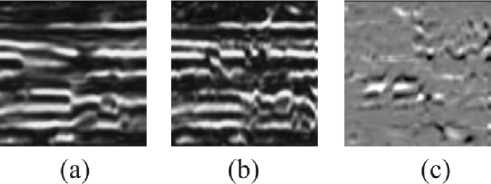
Figure 2: a) Snapshot of the master dynamics recorded with open control loop at $I=3$. a) Space (vertical)-time (horizontal) dynamical evolution of a line of (a) the output free running signal from the MOFL (master dynamics); (b) the slave dynamics in conditions of closed control loop; (c) the synchronization error, corresponding to the difference of (a) and (b). The gray scale in (c) is such that black corresponds to negative values, white to positive values and gray to values close to 0.

With the help of such real-space real-time control technique we have recently given evidence that two dimensional stationary target patterns with arbitrary symmetries and shapes can be effectively and robustly stabilized within STC expnoi . Here, instead, we aim to demonstrating complete synchronization in a unidirectionally coupled scheme between two identical systems in a regime of STC. For this purpose, we initially let the control loop open and record (over a time interval $T$) the free evolution of the system for a value of $I$ at which the uncontrolled dynamics displays STC. A qualitative characterization of the resulting dynamics has been given in expnoi . The signal consists basically of a set of closely packed diffractive spots, evolving in space and time in an unpredictable way.

After the registration of this dynamics, which we refer to as the Master Dynamics (MD) henceforth, further free evolution is granted to the uncontrolled system, so that after a few seconds the configuration of the MOFL output is totally uncorrelated with the initial frame of the MD. At this point, we close the control loop and replay the registered MD as the target pattern $I_{T}(x,y,t)$. In this way, we are implementing a unidirectional coupling scheme between two identical systems starting from fully uncorrelated initial conditions. By repeating the replaying procedure of the MD with increasing values of $\gamma$ (hereinafter called the coupling strength parameter), we eventually observe full synchronization between the controlled output of the MOFL [the slave dynamics (SD)] and the MD.

Complete synchronization between SD and MD is shown in Fig. 2, reporting the space (vertical)-time (horizontal) dynamical evolution of the central vertical line of pixels for the master dynamics (2a), slave dynamics (2b) and the difference between the two, (2c). Fig, 2 is taken at $\gamma=0.8$, and shows how the SD closely follows the MD at any time during control. As visible in fig, 2c, the synchronization error $E(x,y,t)=I_{fb}(x,y,t)-I_{T}(x,y,t)$ is close to vanishing nearly always and everywhere in time as a result of the complete synchronization process.

Notice that the final CS state is here realized within a full STC regime, at variance with what reported in Ref. chemistry for a bidirectional coupling between two excitable media, where the emergence of synchronization was associated with the suppression of space-time chaos in the system.

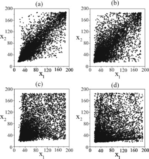
Figure 3: Experimental point distributions in the $(x_{\text{SD}},x_{\text{MD}})$ plane (see text for definition of the variables). The synchronization manifold is represented by the diagonal line $x_{\text{SD}}=x_{\text{MD}}$. (a) $I=2,\ \gamma=0.8$, b) $I=3,\ \gamma=0.8$, c) $I=2,\ \gamma=0$, d) $I=3,\ \gamma=0$.

An independent way of visualizing the emergence of CS is to pick randomly a set of $N$ points [$(x_{i},y_{i});\ i=1,\ldots,N$] in both the MD and the SD, and to plot the variable $x_{\text{SD}}(t)=\left\{I_{fb}(x_{i},y_{i},t),\ \ i=1,\ldots,N\right\}$ vs. the corresponding variable $x_{\text{MD}}(t)=\left\{I_{T}(x_{i},y_{i},t),\ \ i=1,\ldots,N\right\}$. The more the distribution of points in the $(x_{\text{SD}},x_{\text{MD}})$ plane approaches the synchronization manifold (the diagonal line $x_{\text{SD}}=x_{\text{MD}}$), the cleaner a CS state is set in our system at all times. Experimental results are reported in Fig. 3 for two values of the coupling strength $\gamma$. Precisely, Fig. 3a (3c) shows the distribution of points in the $(x_{\text{SD}},x_{\text{MD}})$ plane for $I=2$ and $\gamma=0.8$ ($\gamma=0$), while Fig. 3b (3d) refers to the same situation for $I=3$ and $\gamma=0.8$ ($\gamma=0$). In both cases, it is apparent that increasing the coupling strength induces a point distribution much closer to the diagonal line than the uncoupled case, giving evidence that a CS state has arisen in the experiment.

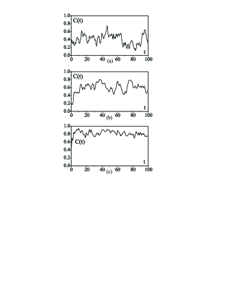
Figure 4: Cross correlation function $C(t)$ (see text for definition) vs. time during some synchronization trials for $I=3$. a) $\gamma=0.24$, b) $\gamma=0.40$, c) $\gamma=0.8$. In all cases $t=0$ indicates the instant at which the MD starts to be replayed in the control loop.

A more quantitative measurement of CS can be given by monitoring the behavior of the time dependent cross-correlation function $C(t)=<I_{fb}(\textbf{r},t)\cdot I_{T}(\textbf{r},t)>_{\textbf{r}}$ between the instantaneous patterns in the SD and MD during the synchronization process ($<\ldots>_{\textbf{r}}$ denotes here a spatial average in the plane ${\textbf{r}}\equiv(x,y)$). $C(t)$ is by definition vanishing for linearly uncorrelated systems, whereas $C(t)\sim 1$ for fully synchronized dynamics.

Fig. 4 reports the temporal behavior of $C(t)$ for $I=3$ and for three different values of the coupling strength [a) $\gamma=0.24$, b) $\gamma=0.4$, and c) $\gamma=0.8$]. In all horizontal axes, $t=0$ has been taken as the instant at which the MD starts to be replayed in the control loop. A first important observation is the cross correlation starts from a non vanishing value at $t=0$. This is because the uncontrolled STC dynamics has a non zero mean field, as it can be appreciated from inspection of Fig. 2a-2b. Namely, the uncoupled MD and SD have a certain degree of ”phase rigidity”, i.e., even if there are chaotic fluctuations, bright (dark) areas remain more or less bright (dark) for most of time. Similar properties have been observed experimentally and discussed in various other cases of space extended systems giving rise to STC dynamics vari .

At low values of the coupling strength ($\gamma=0.24$), no synchronization is set in the system. This is visible in Fig. 4a, where $C(t)$ experiences large fluctuations in time around a mean value not substantially different from the initial correlation level. For intermediate coupling strengths ($\gamma=0.4$ in Fig. 4b), a partial synchronization emerges in the system after a transient time, though several deviations of the SD from the MD still remain, reflected by the rather large fluctuations around the asymptotic value of $C(t)$ visible in Fig. 4b. Finally, a further increase in $\gamma$ induce a full CS in the system (see the case $\gamma=0.8$ in Fig. 4c), where the asymptotic value of the cross correlation approaches unity, and the residual fluctuations in $C(t)$ shrink considerably. Notice that, as $\gamma$ increases, the transient time before reaching CS decreases. The global picture depicted in Fig. 4 confirms that CS here is a threshold phenomenon, as it was introduced originally for time-chaotic systems complete .

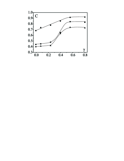
Figure 5: Time average cross correlation function $C$ (see text for definition) vs. the coupling strength $\gamma$ for $I=2$ (circles), $I=3$ (squares), and $I=4$ (triangles). In all cases, the solid lines connecting points are drawn as guides for the eyes.

The global scenario of observed CS is illustrated in Fig. 5, where the time average of the cross correlation function $C=<C(t)>_{T}$ ($<\ldots>_{T}$ here denotes a further time average over the full time interval $T$) is reported vs. the coupling strength at different values of pump intensities $I$. In all cases, our proposed coupling scheme is effective in inducing CS, as $C$ considerably increases with $\gamma$ with respect to the corresponding uncoupled values. An increase in the pump intensity $I$ leads to a progressive deterioration of CS, reflected by smaller asymptotic values of $C(t)$.

In conclusion, we have demonstrated that a unidirectional coupling between two identical pattern forming systems induces complete synchronization of the slave to the master dynamics, with a resulting synchronized behavior corresponding to a spatiotemporal chaotic state. Though realized with a nonlinear optical experiment, the coupling scheme used (based on a real-space real-time control of a recorded and replayed space-time chaotic dynamics) can in principle be implemented in many other physical and chemical pattern forming systems. Furthermore, the great flexibility offered by the proposed coupling scheme can be exploited to drive the slave system onto a generic desired dynamics with arbitrary symmetries and shapes in space, as well as arbitrary behaviors in time.

Work partly supported by MIUR-FIRB project n. RBNE01CW3M-001.

References

- (1) S. Boccaletti, J. Kurths, G. Osipov, D. Valladares and C. Zhou, Phys. Rep. 366, 1, (2002).
- (2) S. Strogatz, ”Sync: The Emerging Science of Spontaneous Order”, Hyperion Press, 2003.
- (3) H. Fujisaka and T. Yamada, Prog. Theor. Phys. 69, 32 (1983); L.M. Pecora and T.L. Carroll, Phys. Rev. Lett. 64, 821 (1990).
- (4) L. Kocarev and U. Parlitz, Phys. Rev. Lett. 76, 1816, (1996).
- (5) M.G. Rosenblum, A.S. Pikovsky and J. Kurths, Phys. Rev. Lett. 76, 1804 (1996).
- (6) M.G. Rosenblum, A.S. Pikovsky and J. Kurths, Phys. Rev. Lett. 78, 4193 (1997); S. Boccaletti and D.L. Valladares, Phys. Rev. E62, 7497 (2000).
- (7) C. Schafer, M.G. Rosemblum, J. Kurths and H.H. Abel, Nature 392, 239 (1998); G. M. Hall, S. Bahar and D.J. Gauthier, Phys. Rev. Lett. 82, 2995 (1999).
- (8) L.M. Pecora and T.L. Carrol, Phys. Rev. Lett. 64, 821 (1990); K.M. Cuomo and A. V. Oppenheim, Phys. Rev. Lett. 71, 65 (1993); R. Roy and K.S. Thornburg, Phys. Rev. Lett. 72, 2009 (1994); D. Maza, A. Vallone, H. Mancini and S. Boccaletti, Phys. Rev. Lett. 85, 5567 (2000); H.B. Pedersen et Al., Phys. Rev. Lett. 87, 055001 (2001).
- (9) R. Brown and L. Kocarev, Chaos 10, 344 (2000); S. Boccaletti, Louis M. Pecora, A. Pelaez, Phys. Rev. E63, 066219 (2001).
- (10) S. H. Strogatz, R.E. Mirollo and P.C. Matthews, Phys. Rev. Lett. 68, 2730 (1992); D.H. Zanette, Phys. Rev. E55, 5315 (1997); V. N. Belykh, I.V. Belykh and M. Hasler, Phys. Rev. E62, 6332 (2000).
- (11) V. N. Belykh and E. Mosekilde, Phys. Rev. E54, 3196 (1996); A. Pikovsky, O. Popovych and Yu. Maistrenko, Phys. Rev. Lett. 87, 044102 (2001).
- (12) H. Gang and QuZhilin, Phys. Rev. Lett. 72, 68 (1994); L. Kocarev, Z. Tasev and U. Parlitz, Phys. Rev. Lett. 79, 51 (1997); S. Boccaletti, J. Bragard, F.T. Arecchi and H. Mancini, Phys. Rev. Lett. 83, 536 (1999).
- (13) M. Hildebrand, J. Cui, E. Mihaliuk, J. Wang and K. Showalter, Phys. Rev. E68, 026205 (2003).
- (14) R. Neubecker and B. Gütlich, Phys. Rev. Lett. 92, 154101 (2004).
- (15) E.A. Rogers, R. Kalra, R.D. Schroll, A. Uchida, D.P. Lathrop and R. Roy, Phys. Rev. Lett. 93, 084101 (2004).
- (16) S.A. Akhmanov, M.A. Vorontsov and V. Yu Ivanov, JETP Lett. 47, 707 (1988).
- (17) G. D’Alessandro and W.J. Firth, Phys. Rev. Lett. 66 2597 (1991).
- (18) R. Neubecker , G.L. Oppo, B. Thuering and T. Tschudi, 1995 Phys. Rev. A52, 791.
- (19) R. Neubecker, B. Thuring, M. Kreuzer and T. Tschudi, Chaos, Solitons and Fractals 10, 681 (1999).
- (20) L. Pastur, L. Gostiaux, U. Bortolozzo, S. Boccaletti, and P. L. Ramazza, Phys. Rev. Lett. 93, 063902 (2004).
- (21) B.J. Gluckman, P. Marcq, J. Bridger and J.P. Gollub, Phys. Rev. Lett. 71, 2034 (1993); Li Ning, Y. Hu, R.E. Ecke and G. Ahlers, Phys. Rev. Lett. 71, 2216 (1993); E. Bosch, H. Lambermont and W. van de Water, Phys. Rev. E49, R3580 (1994); S. Rudroff and I. Rehberg, Phys. Rev. E55, 2742 (1997).