Scalar Decay in Chaotic Mixing

Abstract

I review the local theory of mixing, which focuses on infinitesimal blobs of scalar being advected and stretched by a random velocity field. An advantage of this theory is that it provides elegant analytical results. A disadvantage is that it is highly idealised. Nevertheless, it provides insight into the mechanism of chaotic mixing and the effect of random fluctuations on the rate of decay of the concentration field of a passive scalar.

1 Introduction

The equation that is in the spotlight is the advection–diffusion equation

$$\partial_{t}\theta+{\bm{v}}\cdot\nabla\theta=\kappa\nabla^{2}\theta$$ (1)

for the time-evolution of a distribution of concentration $\theta({\bm{x}},t)$, being advected by a velocity field ${\bm{v}}({\bm{x}},t)$, and diffused with diffusivity $\kappa$. The concentration $\theta$ is called a scalar (as opposed to a vector). We will restrict our attention to incompressible velocity fields, for which $\nabla\cdot{\bm{v}}=0$. For our purposes, we shall leave the exact nature of $\theta$ nebulous: it could be a temperature, the concentration of salt, dye, chemicals, isotopes, or even plankton. The only assumption for now is that this scalar is passive, which means that its value does not affect the velocity field ${\bm{v}}$. Clearly, this is not strictly true of some scalars like temperature, because a varying buoyancy influences the flow, but is often a good approximation nonetheless.

The advection–diffusion equation is linear, but contrary to popular belief that does not mean it is simple! Because the velocity (which is regarded here as a given vector field) is a function of space and time, the advection term (the second term in (1)) can cause complicated behaviour in $\theta$. Broadly speaking, the advection term tends to create sharp gradients of $\theta$, whilst the diffusion term (the term on the right-hand side of (1)) tends to wipe out gradients. The evolution of the concentration field is thus given by a delicate balance of advection and diffusion.

The advection term in (1) is also known as the stirring term, and the interplay of advection and diffusion is often called stirring and mixing. As we shall see, the two terms have very different rôles, but both are needed to achieve an efficient mixing.

To elicit some broad features of mixing, we will start by deriving some properties of the advection–diffusion equation. First, it conserves the total quantity of $\theta$. If we use angle brackets to denote the average of $\theta$ over the fixed domain of interest $V$, i.e.

$$\left\langle\theta\right\rangle\mathrel{\raisebox{0.29707pt}{:}\!\!=}\frac{1}{V}\int_{V}\theta\,{\mathrm{d}}V,$$

then we find diretly from (1) that

$$\partial_{t}\left\langle\theta\right\rangle+\left\langle{\bm{v}}\cdot\nabla\theta\right\rangle=\kappa\left\langle\nabla^{2}\theta\right\rangle.$$ (2)

Because the velocity field is incompressible, we have

$${\bm{v}}\cdot\nabla\theta=\nabla\cdot(\theta\,{\bm{v}}),$$

and also $\nabla^{2}\theta=\nabla\cdot(\nabla\theta)$. Thus, we can use the divergence theorem to write (2) as

$$\partial_{t}\left\langle\theta\right\rangle=-\frac{1}{V}\int_{S}\theta\,{\bm{v}}\cdot\hat{\bm{n}}\,{\mathrm{d}}S+\kappa\,\frac{1}{V}\int_{S}\nabla\theta\cdot\hat{\bm{n}}\,{\mathrm{d}}S,$$ (3)

where $S$ is the surface bounding $V$, and $\,{\mathrm{d}}S$ is the element of area, and $\hat{\bm{n}}$ outward-pointing normal to the surface. For a closed flow, two possibilities are now open to us: (i) the domain $V$ is periodic; or (ii) ${\bm{v}}$ and $\nabla\theta$ are both tangent to the surface $S$. In the first case, the terms on the right-hand side of (3) vanish because boundary terms always vanish with periodic boundary conditions (a bit tautological, but true!). In the second case, both ${\bm{v}}\cdot\hat{\bm{n}}$ and $\nabla\theta\cdot\hat{\bm{n}}$ vanish. Either way,

$$\partial_{t}\left\langle\theta\right\rangle=0$$ (4)

so that the mean value of $\theta$ is constant. Since $V$ is constant, this also implies that the total amount of $\theta$ is conserved. The second set of boundary conditions we used implies that there is no fluid flow or flux of $\theta$ through the boundary of the volume. It is thus natural that the total $\theta$ is conserved! For periodic boundary conditions, whatever leaves the volume re-enters on the other side, so it also makes sense that $\theta$ is conserved. Because of (4), and because we can always add a constant to $\theta$ without changing its evolution (only derivatives of $\theta$ appear in (1)), we will always choose

$$\left\langle\theta\right\rangle=0$$ (5)

without loss of generality. In words: the mean of our scalar vanishes initially, so by (4) it must vanish for all times.

Now let’s look at another average of $\theta$: rather than averaging $\theta$ itself, which has yielded an important but boring result, we average its square. The variance is defined by

$$\mathrm{Var}\mathrel{\raisebox{0.29707pt}{:}\!\!=}\langle\theta^{2}\rangle-\langle\theta\rangle^{2},$$ (6)

where the second term on the right vanishes by (5). To obtain an equation for the time-evolution of the variance, we multiply (1) by $\theta$ and integrate,

$$\left\langle\theta\,\partial_{t}\theta\right\rangle+\left\langle\theta\,{\bm{v}}\cdot\nabla\theta\right\rangle=\kappa\left\langle\theta\,\nabla^{2}\theta\right\rangle.$$

We rearrange on the left and integrate by parts on the right, to find

$$\left\langle\left(\partial_{t}+{\bm{v}}\cdot\nabla\right)\tfrac{1}{2}\,\theta^{2}\right\rangle=\kappa\left\langle\nabla\cdot(\theta\,\nabla\theta)-\lvert\nabla\theta\rvert^{2}\right\rangle.$$

Now there are some boundary terms that vanish under the same assumptions as before, and we get

$$\partial_{t}\mathrm{Var}=-2\kappa\left\langle\lvert\nabla\theta\rvert^{2}\right\rangle.$$ (7)

Notice that, once again, the velocity field has dropped out of this averaged equation. However, now the effect of diffusion remains. Moreover, it is clear that the term on the right-hand side of (7) is negative-definite (or zero): this means that the variance always decreases (or is constant). The only way it can stop decreasing is if $\nabla\theta$ vanishes everywhere, that is, $\theta$ is constant in space. But because we have assumed $\left\langle\theta\right\rangle=0$, this means that $\theta=0$ everywhere. In that case, we have no choice but to declare the system to be perfectly mixed: there are no variations in $\theta$ at all anymore. Equation (7) tells us that variance tends to zero, which means that the system inexorably tends to the perfectly mixed state, without necessarily ever reaching it. Variance is thus a useful measure of mixing: the smaller the variance, the better the mixing.

There is a problem with all this: equation (7) no longer involves the velocity field. But if variance is to give us a measure of mixing, shouldn’t its time-evolution involve the velocity field? Is this telling us that stirring has no effect on mixing? Of course not, as any coffee-drinker will testify, whether she likes it with milk or sugar: stirring has a huge impact on mixing! So what’s the catch?

The catch is that (7) is not a closed equation for the variance: the right-hand side involves $\lvert\nabla\theta\rvert^{2}$, which is not the same as $\theta^{2}$. The extra gradient makes all the difference. As we will see, under the right circumstances the stirring velocity field creates very large gradients in the concentration field, which makes variance decrease much faster than it would if diffusivity were acting alone. In fact, when $\kappa$ is very small, in the best stirring flows the gradients of $\theta$ scale as $\kappa^{-1/2}$, so that the right-hand side of (7) becomes independent of the diffusivity. This, in a nutshell, is the essence of enhanced mixing.

Several important questions can now be raised:

• How fast is the approach to the perfectly-mixed state?

• How does this depend on $\kappa$?

• What does the concentration field look like for long times? What is its spectrum?

• How does the probability distribution of $\theta$ evolve?

• Which stirring fields give efficient mixing?

The answers to these questions are quite complicated, and not fully known. In the following sections we will attempt to give some hints of the answers and give some references to the literature.

This is not meant to be a comprehensive review article, so entire swaths of the literature are missing. We focus mainly on local or Lagrangian theories, which involve deterministic and stochastic approaches for quantifying stretching using a local idealisation of the flow. The essential feature here is that the advection–diffusion equation is solved along fluid trajectories. These theories trace their origins to Batchelor Batchelor1959 , who treated constant matrices with slow time dependence, and Kraichnan, who introduced fast (delta-correlated) time dependence Kraichnan1968 ; Kraichnan1974 . Zeldovich et al. Zeldovich1984 approached the problem from the random-matrix theory angle in the magnetic dynamo context. More recently, techniques from large-deviation theory Ott1989 ; Antonsen1991 ; Antonsen1995 ; Antonsen1996 and path integration Shraiman1994 ; Chertkov1995 ; Chertkov1997 ; Shraiman2000 ; Falkovich2001 have allowed an essentially complete solution of the problem. It is this work that will be reviewed here, as it applies to the decay of the passive scalar (and not the PDF of concentration or its power spectrum). We will favour expediency over mathematical rigour, and try to give a flavour of what these local theories are about without describing them in detail.

The story will proceed from here as follows: in Section 2 advection of a blob by a linear velocity field is considered, with diffusion included. This problem has an exact solution, but it can be made simpler in the limit of small diffusivity. Solutions are examined for a straining flow in two and three dimensions (Sections 2.2 and 2.4), as well as a shear flow in two dimensions (Section 2.3). Randomness is added in Section 3: the strain associated with the velocity field is assumed to vary, and the consequences of this for a single blob (Section 3.1) and a large number of blobs (Section 3.2) are explored. Practical implementation is discussed in Section 4, and a simple model for a micromixer is analysed in Section 4.1. Finally, the limitations of the theory presented herein (Section 4.2).

2 Advection and Diffusion in a Linear Velocity Field

We will start by considering what happens to a passive scalar advected by a linear velocity field. The overriding advantage of this configuration is that it can be solved analytically, but that is not its only pleasant feature. Like most good toy models, it serves as a nice prototype for what happens in more complicated flows. It also serves as a building block for what may be called the local theory of mixing (Section 3).

The perfect setting to consider a linear flow is in the limit of large Schmidt number. The Schmidt number is a dimensionless quantity defined as

$$\mathrm{Sc}\mathrel{\raisebox{0.29707pt}{:}\!\!=}\nu/\kappa$$

where $\nu$ is the kinematic viscosity of the fluid and $\kappa$ is the diffusivity of the scalar. The Schmidt number may be thought of as the ratio of the diffusion time for the scalar to that for momentum in the fluid. Alternatively, it can be regarded as the ratio of the (squared) length of the smallest feature in the velocity field to that in the scalar field. This last interpretation is due to the fact that if $\theta$ varies in space more quickly than $\sqrt{\kappa}$, then its gradient is large and diffusion wipes out the variation. The same applies to variations in the velocity field with respect to $\nu$. Hence, for large Schmidt number the scalar field has much faster variations than the velocity field. This means that it is possible to focus on a region of the domain large enough for the scalar concentration to vary appreciably, but small enough that the velocity field appears linear. Because there are many cases for which $\mathrm{Sc}$ is quite large, this motivates the use of a linear velocity field. In fact, large $\mathrm{Sc}$ number is the natural setting for chaotic advection. It is also the regime that was studied by Batchelor and leads to the celebrated Batchelor spectrum Batchelor1959 . The limit of small $\mathrm{Sc}$ is the domain of homogenization theory and of turbulent diffusivity models. We shall not discuss such things here.

2.1 Solution of the Problem

We choose a linear velocity field of the form

$${\bm{v}}={\bm{x}}\cdot\sigma(t),\qquad\operatorname{Tr}\sigma=0,$$

where $\sigma$ is a traceless matrix because $\nabla\cdot{\bm{v}}$ must vanish. Inserting this into (1), we want to solve the initial value problem

$$\partial_{t}\theta+{\bm{x}}\cdot\sigma(t)\cdot\nabla\theta=\kappa\nabla^{2}\theta,\qquad\theta({\bm{x}},0)=\theta_{0}({\bm{x}}).$$ (8)

Here the coordinate ${\bm{x}}$ is really a deviation from a reference fluid trajectory. (In Appendix 5 we derive (8) from (1) by transforming to a comoving frame and assuming the velocity field is smooth.) We will follow closely the solution of Zeldovich et al. Zeldovich1984 , who solved this by the method of “partial solutions.” Consider a solution of the form

$$\theta({\bm{x}},t)=\hat{\theta}({\bm{k}}_{0},t)\exp(\mathrm{i}{\bm{k}}(t)\cdot{\bm{x}}),\qquad{\bm{k}}(0)={\bm{k}}_{0},\quad\hat{\theta}({\bm{k}}_{0},0)=\hat{\theta}_{0}({\bm{k}}_{0}),$$ (9)

where ${\bm{k}}_{0}$ is some initial wavevector. We will see if we can make this into a solution by a judicious choice of $\hat{\theta}({\bm{k}}_{0},t)$ and ${\bm{k}}(t)$. The time derivative of (9) is

$$\partial_{t}\theta=(\partial_{t}\hat{\theta}+\mathrm{i}\,\partial_{t}{\bm{k}}\cdot{\bm{x}}\,\hat{\theta})\exp(\mathrm{i}{\bm{k}}(t)\cdot{\bm{x}})$$

and we have

$${\bm{v}}\cdot\nabla\theta=\mathrm{i}\,({\bm{x}}\cdot\sigma\cdot{\bm{k}})\,\hat{\theta}\exp(\mathrm{i}{\bm{k}}(t)\cdot{\bm{x}}).$$

Putting these together into (8) and cancelling out the exponential gives

$$\partial_{t}\hat{\theta}+\mathrm{i}\,{\bm{x}}\cdot(\partial_{t}{\bm{k}}+\sigma\cdot{\bm{k}})\,\hat{\theta}=-\kappa\,k^{2}\hat{\theta}.$$

This must hold for all ${\bm{x}}$, and neither $\hat{\theta}$ nor ${\bm{k}}$ depend on ${\bm{x}}$, so we equate powers of ${\bm{x}}$. This gives the two evolution equations

$$\partial_{t}{\bm{k}} =-\sigma\cdot{\bm{k}}\,,$$ (10a)

$$\partial_{t}\hat{\theta} =-\kappa\,k^{2}\hat{\theta}.$$ (10b)

We can write the solution to (10a) in terms of the fundamental solution $\mathcal{T}(t,0)$ as

$${\bm{k}}(t)=\mathcal{T}(t,0)\cdot{\bm{k}}_{0}\,,$$

where

$$\partial_{t}\mathcal{T}(t,0)=-\sigma(t)\cdot\mathcal{T}(t,0),\qquad\mathcal{T}(0,0)=\mathrm{Id}$$ (11)

and $\mathrm{Id}$ is the identity matrix. The advantage of doing this is that we can use the same fundamental solution for all initial conditions. We will usually write $\mathcal{T}_{t}$ to mean $\mathcal{T}(t,0)$. Note that because $\operatorname{Tr}\sigma=0$, we have

$$\det\mathcal{T}_{t}=1.$$ (12)

This is a standard result that is proved in Appendix 6 for completeness. If $\sigma$ is not a function of time, then the fundamental solution is simply a matrix exponential,

$$\mathcal{T}_{t}=\exp(-\sigma\,t),$$

but in general the form of $\mathcal{T}_{t}$ is more complicated.

Now that we know the time-dependence of ${\bm{k}}$, we can express the solution to (10) as

$${\bm{k}}(t) =\mathcal{T}_{t}\cdot{\bm{k}}_{0}\,,$$ (13a)

$$\hat{\theta}({\bm{k}}_{0},t) =\hat{\theta}_{0}({\bm{k}}_{0})\exp\left\{-\kappa\int_{0}^{t}\bigl{(}\mathcal{T}_{s}\cdot{\bm{k}}_{0}\bigr{)}^{2}\,{\mathrm{d}}s\right\}.$$ (13b)

We can think of $\mathcal{T}_{t}$ as transforming a Lagrangian wavevector ${\bm{k}}_{0}$ to its Eulerian counterpart ${\bm{k}}$. Thus (13b) expresses the fact that $\hat{\theta}$ decays diffusively at a rate determined by the cumulative norm of the wavenumber ${\bm{k}}$ experienced during its evolution.

The full solution to (8) is now given by superposition of the partial solutions,

$$\theta({\bm{x}},t) =\int\hat{\theta}({\bm{k}}_{0},t)\exp(\mathrm{i}{\bm{k}}(t)\cdot{\bm{x}})\,{\mathrm{d}}^{3}k_{0}$$

$$=\int\hat{\theta}_{0}({\bm{k}}_{0})\exp\left\{\mathrm{i}\,{\bm{x}}\cdot\mathcal{T}_{t}\cdot{\bm{k}}_{0}-\kappa\int_{0}^{t}\bigl{(}\mathcal{T}_{s}\cdot{\bm{k}}_{0}\bigr{)}^{2}\,{\mathrm{d}}s\right\}\!\,{\mathrm{d}}^{3}k_{0}\,,$$ (14)

where $\hat{\theta}_{0}({\bm{k}}_{0})$ is the Fourier transform of the initial condition $\theta_{0}({\bm{x}})$. Assuming the spatial mean of $\theta$ vanishes, the variance (6) is

$$\mathrm{Var}=\int\theta^{2}({\bm{x}},t)\,{\mathrm{d}}^{3}x=\int\lvert\hat{\theta}({\bm{k}}_{0},t)\rvert^{2}\,{\mathrm{d}}^{3}k_{0}\,,$$

which from (13b) becomes

$$\mathrm{Var}=\int\lvert\hat{\theta}_{0}({\bm{k}}_{0})\rvert^{2}\exp\left\{-2\kappa\int_{0}^{t}\bigl{(}\mathcal{T}_{s}\cdot{\bm{k}}_{0}\bigr{)}^{2}\,{\mathrm{d}}s\right\}\!\,{\mathrm{d}}^{3}k_{0}\,.$$ (15)

We thus have a full solution of the advection–diffusion equation for the case of a linear velocity field and found the time-evolution of the variance. But what can be gleaned from it? We shall look at some special cases in the following section.

2.2 Straining Flow in 2D

We now take an even more idealised approach: consider the case where the velocity gradient matrix $\sigma$ is constant. Furthermore, let us restrict ourselves to two-dimensional flows. After a coordinate change, the traceless matrix $\sigma$ can only take two possible forms,

$$\sigma^{\text{(2a)}}=\begin{pmatrix}\lambda&0\\ 0&-\lambda\end{pmatrix}\qquad\text{and}\qquad\sigma^{\text{(2b)}}=\begin{pmatrix}0&0\\ U^{\prime}&0\end{pmatrix}.$$ (16)

Case (2a) is a purely straining flow that stretches exponentially in one direction, and contracts in the other. Case (2b) is a linear shear flow in the $x_{1}$ direction. We assume without loss of generality that $\lambda>0$ and $U^{\prime}>0$. The form $\sigma^{(2b)}$ is known as the Jordan canonical form, and can only occur for degenerate eigenvalues. Since by incompressibility the sum of these identical eigenvalues must vanish, they must both vanish. The corresponding fundamental matrices $\mathcal{T}_{t}=\exp(-\sigma\,t)$ are

$$\mathcal{T}_{t}^{\text{(2a)}}=\begin{pmatrix}{\mathrm{e}}^{-\lambda t}&0\\ 0&{\mathrm{e}}^{\lambda t}\end{pmatrix}\qquad\text{and}\qquad\mathcal{T}_{t}^{\text{(2b)}}=\begin{pmatrix}1&0\\ -U^{\prime}t&1\end{pmatrix}.$$ (17)

These are easy to compute: in the first instance one merely exponentiates the diagonal elements, in the second the exponential power series terminates after two terms, because the square of $\sigma^{(2b)}$ is zero.

Let us consider Case (2a), a flow with constant stretching (the case considered by Batchelor Batchelor1959 ). The action of the fundamental matrix on ${\bm{k}}_{0}$ for Case (2a) is

$$\mathcal{T}^{(2a)}_{t}\cdot{\bm{k}}_{0}=\left({\mathrm{e}}^{-\lambda t}\,{k_{0}}_{1}\,,\,{\mathrm{e}}^{\lambda t}\,{k_{0}}_{2}\right),$$ (18)

with norm

$$\bigl{(}\mathcal{T}^{(2a)}_{t}\cdot{\bm{k}}_{0}\bigr{)}^{2}={\mathrm{e}}^{-2\lambda t}\,{k_{0}}_{1}^{2}+{\mathrm{e}}^{2\lambda t}\,{k_{0}}_{2}^{2}\,.$$ (19)

The wavevector ${\bm{k}}(t)=\mathcal{T}^{(2a)}_{t}\cdot{\bm{k}}_{0}$ grows exponentially in time, which means that the length scale is becoming very small. This only occurs in the direction $x_{2}$, which is sensible because that direction corresponds to a contracting flow. Picture a curtain being closed: the bunching up of the fabric into tight folds is analogous to the contraction. (Of course, it is difficult to close a curtain exponentially quickly forever!) The component of the wavevector in the $x_{1}$ direction decreases in magnitude, which corresponds to the opening of a curtain.

Let’s see what happens to one Fourier mode. By inserting (19) in (13b), we have

$$\hat{\theta}({\bm{k}}_{0},t)=\hat{\theta}_{0}({\bm{k}}_{0})\exp\left\{-\kappa\int_{0}^{t}\bigl{(}{\mathrm{e}}^{-2\lambda s}\,{k_{0}}_{1}^{2}+{\mathrm{e}}^{2\lambda s}\,{k_{0}}_{2}^{2}\bigr{)}\,{\mathrm{d}}s\right\}\,.$$

The time-integral can be done explicitly, and we find

$$\hat{\theta}({\bm{k}}_{0},t)=\hat{\theta}_{0}({\bm{k}}_{0})\exp\left\{-\frac{\kappa}{2\lambda}\left(\left({\mathrm{e}}^{2\lambda t}-1\right){k_{0}}_{2}^{2}-\left({\mathrm{e}}^{-2\lambda t}-1\right){k_{0}}_{1}^{2}\right)\right\}\,.$$

For moderately long times ($t\gtrsim\lambda^{-1}$), we can surely neglect ${\mathrm{e}}^{-2\lambda t}$ compared to $1$, and $1$ compared to ${\mathrm{e}}^{2\lambda t}$,

$$\hat{\theta}({\bm{k}}_{0},t)\simeq\hat{\theta}_{0}({\bm{k}}_{0})\exp\left\{-\frac{\kappa}{2\lambda}\left({\mathrm{e}}^{2\lambda t}\,{k_{0}}_{2}^{2}+{k_{0}}_{1}^{2}\right)\right\}\,.$$ (20)

Actually, this assumption of moderately long time is easily justified physically. If $\kappa k^{2}/\lambda\ll 1$, where $k$ is the largest initial wavenumber (that is, the smallest initial scale), then the argument of the exponential in (20) is small, unless

$${\mathrm{e}}^{2\lambda t}\gtrsim\mathrm{Pe}$$ (21)

where the Péclet number is

$$\mathrm{Pe}=\frac{\lambda}{\kappa\,k^{2}}\,.$$ (22)

Thus the assumption that ${\mathrm{e}}^{2\lambda t}$ is large is a consequence of $\mathrm{Pe}$ being large, since otherwise the exponential in (20) is near unity and can be ignored—variance is approximately constant. We can turn (21) into a requirement on the time,

$$\lambda\,t\gtrsim\log\mathrm{Pe}^{1/2}\,.$$ (23)

It is clear from (23) that $\lambda^{-1}$ sets the time scale for the argument of the exponential in (20) to become important. The Péclet number influences this time scale only weakly (logarithmically). This is probably the most important physical fact about chaotic mixing: Small diffusivity has only a logarithmic effect. Thus vigorous stirring always has a chance to overcome a small diffusivity, no matter how small: we need just stir a bit longer.

Note that the variance is given by

$$\mathrm{Var}=\int\lvert\hat{\theta}_{0}({\bm{k}}_{0})\rvert^{2}\exp\left\{-\frac{\kappa}{\lambda}\left({\mathrm{e}}^{2\lambda t}\,{k_{0}}_{2}^{2}+{k_{0}}_{1}^{2}\right)\right\}\!\,{\mathrm{d}}^{2}k_{0}\,,$$

which is approximately constant for $t\ll\lambda^{-1}\log\mathrm{Pe}^{1/2}$. This does not mean that the concentration field

$$\theta({\bm{x}},t)=\int\hat{\theta}({\bm{k}}_{0},t)\,{\mathrm{e}}^{\mathrm{i}{\bm{k}}(t)\cdot{\bm{x}}}\,{\mathrm{d}}^{2}k_{0}$$ (24)

is constant, even if $\hat{\theta}({\bm{k}}_{0},t)$ is, because ${\bm{k}}(t)=\mathcal{T}^{(2a)}_{t}\cdot{\bm{k}}_{0}$ is a function of time from (18). This time dependence becomes important for $t\gtrsim\lambda^{-1}$.

The Péclet number may be thought of as the ratio of the advection time of the flow to the diffusion time for the scalar. It is usually written as

$$\mathrm{Pe}\mathrel{\raisebox{0.29707pt}{:}\!\!=}UL/\kappa\,,$$ (25)

where $U$ is a typical velocity and $L$ a typical length scale. Our velocity estimate in (22) is $\lambda/k$, and our length scale is $k$, which are both natural for the problem at hand. Just like large $\mathrm{Sc}$, large $\mathrm{Pe}$ is the natural setting for chaotic advection. In fact, if $\mathrm{Pe}$ is small then diffusion is faster than advection, and stirring is not really required! Large $\mathrm{Pe}$ means that diffusion by itself is not very effective, so that stirring is required. We shall always assume that $\mathrm{Pe}$ is large.

We return to (20): the striking thing about that equation is its prediction for the rate of decay of the concentration field. Roughly speaking, (20) predicts

$$\theta({\bm{x}},t)\sim\exp\left\{-\mathrm{Pe}^{-1}\,{\mathrm{e}}^{2\lambda t}\right\}$$ (26)

for $\lambda t\gg 1$. Eq. (26) is the exponential of an exponential—a superexponential decay. This is extremely fast decay. In fact, unnaturally so: it is hard to imagine a physically sensible system that could mix this quickly. Something more has to be at work here.

If we examine (20) closely, we see that the culprit is the term

$${\mathrm{e}}^{2\lambda t}\,{k_{0}}_{2}^{2}\,,$$ (27)

which grows exponentially fast. This term has its origin in the Laplacian in the advection–diffusion equation (1): the contracting direction of the flow (the $x_{2}$ direction) leads to an exponential increase in the wavenumber via the curtain-closing mechanism. This is exactly the mechanism for enhanced mixing we advertised on p. 1: very large gradients of concentration are being created, exponentially fast. This mechanism is just acting too quickly for our taste!

So what’s the problem? We are doing the wrong thing to obtain our estimate (26). This estimate tells us how fast a typical wavevector decays, and it says that this occurs very quickly. What we really want to know is what modes survive superexponential decay the longest, and at what rate they decay. Clearly the concentration in most wavenumbers gets annihilated almost instantly, once the condition (23) is satisfied. But a small number remains: those are the modes with wavevector closely aligned to the $x_{1}$ (stretching) direction, or equivalently that have a very small projection on the $x_{2}$ (contracting) direction. To overcome the exponential growth in (27), we require

$${k_{0}}_{2}\sim{\mathrm{e}}^{-\lambda t}\,,$$ (28)

that is at any given time we need consider only wavenumbers satisfying (28), since the concentration in all the others has long since been wiped out by diffusion. The consequence is that the ${k_{0}}_{2}$ integral in (24) is dominated by these surviving modes. To see this, we blow up the ${k_{0}}_{2}$ integration by making the coordinate change ${{\widetilde{k}}_{0}{}}_{2}={k_{0}}_{2}\,{\mathrm{e}}^{\lambda t}$ in (24),

$$\theta({\bm{x}},t)={\mathrm{e}}^{-\lambda t}\int_{-\infty}^{\infty}\,{\mathrm{d}}{k_{0}}_{1}\int_{-\infty}^{\infty}\,{\mathrm{d}}{{\widetilde{k}}_{0}{}}_{2}\,\,\hat{\theta}_{0}({k_{0}}_{1},{{\widetilde{k}}_{0}{}}_{2}\,{\mathrm{e}}^{-\lambda t})\\ \times\,{\mathrm{e}}^{\mathrm{i}{\bm{k}}(t)\cdot{\bm{x}}}\exp\left\{-\frac{\kappa}{2\lambda}\left({{\widetilde{k}}_{0}{}}_{2}^{2}+{k_{0}}_{1}^{2}\right)\right\},$$ (29)

The decay factor ${\mathrm{e}}^{-\lambda t}$ has appeared in front. For small diffusivity, we can neglect the ${k_{0}}_{1}^{2}$ term in the exponential (it just smooths out the initial concentration field a little). We can then take the inverse Fourier transform of $\hat{\theta}_{0}({k_{0}}_{1},{{\widetilde{k}}_{0}{}}_{2}\,{\mathrm{e}}^{-\lambda t})$,

$$\hat{\theta}_{0}({k_{0}}_{1},{{\widetilde{k}}_{0}{}}_{2}\,{\mathrm{e}}^{-\lambda t})=\frac{1}{(2\pi)^{2}}\int\theta_{0}(\tilde{}{\bm{x}})\,\exp\left(-\mathrm{i}{k_{0}}_{1}\tilde{}x_{1}-\mathrm{i}{{\widetilde{k}}_{0}{}}_{2}\,{\mathrm{e}}^{-\lambda t}\tilde{}x_{2}\right)\,{\mathrm{d}}\tilde{}x_{1}\,{\mathrm{d}}\tilde{}x_{2}$$

and insert this into (29). We then interchange the order of integration: the ${k_{0}}_{1}$ integral gives a $\delta$-function, and the ${{\widetilde{k}}_{0}{}}_{2}$ integral gives a Gaussian. The final result is

$$\theta({\bm{x}},t)={\mathrm{e}}^{-\lambda t}\int_{-\infty}^{\infty}\,\,\theta_{0}({\mathrm{e}}^{-\lambda t}x_{1},\tilde{}x_{2})\,G\bigl{(}x_{2}-{\mathrm{e}}^{-\lambda t}\,\tilde{}x_{2}\,;\,\ell\bigr{)}\,{\mathrm{d}}\tilde{}x_{2}\,,$$ (30)

where

$$G(x;\ell)\mathrel{\raisebox{0.29707pt}{:}\!\!=}\frac{1}{\sqrt{2\pi\ell^{2}}}\,{\mathrm{e}}^{-x^{2}/2\ell^{2}}$$ (31)

is a normalised Gaussian distribution with standard deviation $\ell$, and we defined the length

$$\ell\mathrel{\raisebox{0.29707pt}{:}\!\!=}\sqrt{{\kappa}/{\lambda}}\,.$$

If the initial concentration decays for large $\lvert x_{2}\rvert$ (as when we have a single blob of dye), then (30) can be simplified to

$$\theta({\bm{x}},t)={\mathrm{e}}^{-\lambda t}\,G\bigl{(}x_{2}\,;\,\ell\bigr{)}\int_{-\infty}^{\infty}\,\,\theta_{0}({\mathrm{e}}^{-\lambda t}x_{1},\tilde{}x_{2})\,{\mathrm{d}}\tilde{}x_{2}\,.$$ (32)

So the $x_{1}$ dependence in (32) is given by the “stretched” initial distribution, averaged over $x_{2}$. The important thing to notice is that

$$\theta({\bm{x}},t)\sim{\mathrm{e}}^{-\lambda t}\,.$$ (33)

This is a much more reasonable estimate for the decay of concentration than (26)! The concentration thus decays exponentially at a rate given by the rate-of-strain (or stretching rate) in our flow. The exponential decay is entirely due to the narrowing of the domain for eligible (i.e., nondecayed) modes. This “domain of eligibility” is also known as the cone or the cone of safety Zeldovich1984 ; Thiffeault2004b . (In two dimensions it is more properly called a wedge.) The concentration associated with wavevectors that fit within this cone is temporarily shielded from being diffusively wiped out, but as the aperture of the cone is shrinking exponentially more and more modes leave the safety of the cone as time progresses.

Notice that (33) is independent of $\kappa$. This brings us to the second most important physical fact about chaotic mixing: The asymptotic decay rate of the concentration field tends to be independent of diffusivity. But note that a nonzero diffusivity is crucial in forcing the alignment (28). The only effect of the diffusivity is to lengthen the wait before exponential decay sets in, as given by the estimate (23). But this effect is only logarithmic in the diffusivity.

We can also try to think of (32) in real rather than Fourier space. Consider an initial distribution of concentration. Our straining flow will stretch this distribution in the $x_{1}$ direction, and contract it in the $x_{2}$ direction. Gradients in $x_{2}$ will thus become very large, so that eventually diffusion will limit further contraction in the $x_{2}$ direction and the distribution will stabilise with width $\sqrt{\kappa/\lambda}$ (see Fig. 1). This is what the Gaussian prefactor in (32) is telling us: the asymptotic distribution has “forgotten” its initial shape in $x_{2}$. We say that the contracting direction has been stabilised.

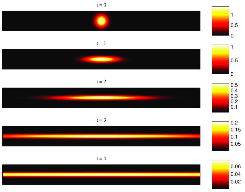
Figure 1: A patch of dye in a uniform straining flow. The amplitude of the concentration field decreases exponentially with time. The length of the filament increases exponentially, whilst its width is stabilised at $\ell=\sqrt{\kappa/\lambda}$.

2.3 Shear Dispersion in 2D

So far we have only considered case (2a) in (16). For case (2b), we have from (17)

$$\mathcal{T}^{(2b)}_{t}\cdot{\bm{k}}_{0}=\left({k_{0}}_{1},{k_{0}}_{2}-U^{\prime}t\,{k_{0}}_{1}\right)$$

with norm

$$\bigl{(}\mathcal{T}^{(2b)}_{t}\cdot{\bm{k}}_{0}\bigr{)}^{2}={k_{0}}_{1}^{2}+\left({k_{0}}_{2}-U^{\prime}t\,{k_{0}}_{1}\right)^{2}\,.$$ (34)

Inserting (34) in (14), we have

$$\theta({\bm{x}},t)=\int\hat{\theta}_{0}({\bm{k}}_{0})\,{\mathrm{e}}^{\mathrm{i}{\bm{k}}(t)\cdot{\bm{x}}}\exp\left\{-\kappa\int_{0}^{t}\bigl{(}{k_{0}}_{1}^{2}+\left({k_{0}}_{2}-U^{\prime}s\,{k_{0}}_{1}\right)^{2}\bigr{)}\,{\mathrm{d}}s\right\}\!\,{\mathrm{d}}^{2}k_{0}\,.$$

We can then explicitly do the time integral in the exponential,

$$\theta({\bm{x}},t)=\int\hat{\theta}_{0}({\bm{k}}_{0})\,{\mathrm{e}}^{\mathrm{i}{\bm{k}}(t)\cdot{\bm{x}}}\\ \times\exp\left\{-\kappa\,{k_{0}}_{1}^{2}\,t-\frac{\kappa}{3U^{\prime}{k_{0}}_{1}}\,\bigl{(}\left(U^{\prime}t\,{k_{0}}_{1}-{k_{0}}_{2}\right)^{3}+{k_{0}}_{2}^{3}\bigr{)}\right\}\!\,{\mathrm{d}}^{2}k_{0}\,.$$ (35)

The enhancement to diffusion in this case is reflected in the cubic power of time in the exponential. This is not as strong as the exponential enhancement of case (2a), but is nevertheless very significant. This phenomenon is known as shear dispersion or Taylor dispersion. The mechanism is often called the venetian blind effect. Assuming the initial distribution $\theta_{0}$ depends only on ${k_{0}}_{1}$, then lines of constant concentration which are initially vertical are tilted by the shear flow, in a manner reminiscent of venetian blinds. The distance between the lines of constant concentration decreases with time as $(U^{\prime}t)^{-1}$, which gives an effective enhancement to diffusion. The time required to overcome a weak diffusivity is thus

$$U^{\prime}t\gtrsim({k_{0}}_{1}^{2}\,\kappa/U^{\prime})^{-1/3}.$$ (36)

If we use ${k_{0}}_{1}^{-1}$ as a length scale and $U^{\prime}$ as a time scale, we can define a Péclet number $\mathrm{Pe}\mathrel{\raisebox{0.29707pt}{:}\!\!=}U^{\prime}/({k_{0}}_{1}{}^{2}\,\kappa)$ and rewrite (36) as

$$U^{\prime}t\gtrsim\mathrm{Pe}^{1/3}$$ (37)

which should be compared to (23), the corresponding expression for the case (2a). Here there is a power law dependence on the Péclet number, rather than logarithmic, so we may have to wait a long time for diffusion to become important. This makes the linear velocity field approximation more likely to break down.

Let us consider the time-asymptotic limit $U^{\prime}t\gg 1$: we might then be tempted to neglect everything but the $U^{\prime}t\,{k_{0}}_{1}$ term in the argument of the exponential in (35). However, this would be a mistake. To see more clearly what happens, define the dimensionless time $\tau\mathrel{\raisebox{0.29707pt}{:}\!\!=}U^{\prime}t$ and the length $\chi^{2}=\kappa/U^{\prime}$. Equation (35) then becomes

$$\theta({\bm{x}},t)=\int\hat{\theta}_{0}({\bm{k}}_{0})\,{\mathrm{e}}^{\mathrm{i}{\bm{k}}(t)\cdot{\bm{x}}}\\ \times\exp\left\{-\chi^{2}\left({k_{0}}_{1}^{2}\tau+{k_{0}}_{2}^{2}\tau+\tfrac{1}{3}{k_{0}}_{1}^{2}\tau^{3}-{k_{0}}_{1}{k_{0}}_{2}\tau^{2}\right)\right\}\!\,{\mathrm{d}}^{2}k_{0}\,.$$ (38)

The first two terms in the exponential are just what is expected of regular diffusion in the absence of flow. The next term is the enhancement to diffusion along the $x_{1}$ direction: it will force the modes ${k_{0}}_{1}\sim\tau^{-3/2}$ to be dominant, since everything else will be damped away. Similarly, the last term forces ${k_{0}}_{2}\sim\tau^{-1/2}$. Assuming these scalings, the only term that can be neglected for $\tau\gg 1$ is the very first one, ${k_{0}}_{1}^{2}\tau$.

We make the change of variable ${{\widetilde{k}}_{0}{}}_{1}=\tau^{3/2}{k_{0}}_{1}$, ${{\widetilde{k}}_{0}{}}_{2}=\tau^{1/2}{k_{0}}_{2}$ in (38),

$$\theta({\bm{x}},t)=\tau^{-2}\int\hat{\theta}_{0}({{\widetilde{k}}_{0}{}}_{1}\,\tau^{-3/2}\,,\,{{\widetilde{k}}_{0}{}}_{2}\,\tau^{-1/2})\,{\mathrm{e}}^{\mathrm{i}(\tau^{-3/2}x_{1}-\tau^{-1/2}x_{2}){{\widetilde{k}}_{0}{}}_{1}+\mathrm{i}\tau^{-1/2}x_{2}{{\widetilde{k}}_{0}{}}_{2}}\\ \times\exp\left\{-\chi^{2}\left({{\widetilde{k}}_{0}{}}_{2}^{2}+\tfrac{1}{3}{{\widetilde{k}}_{0}{}}_{1}^{2}-{{\widetilde{k}}_{0}{}}_{1}{{\widetilde{k}}_{0}{}}_{2}\right)\right\}\!\,{\mathrm{d}}{{\widetilde{k}}_{0}{}}_{1}\,{\mathrm{d}}{{\widetilde{k}}_{0}{}}_{2}\,.$$ (39)

If we approximate $\hat{\theta}_{0}({{\widetilde{k}}_{0}{}}_{1}\,\tau^{-3/2}\,,\,{{\widetilde{k}}_{0}{}}_{2}\,\tau^{-1/2})\simeq\hat{\theta}_{0}(0,0)$, we can do the integrals in (39) and find

$$\theta({\bm{x}},t)\simeq 2\sqrt{3}\pi\,\chi^{-2}\,\tau^{-2}\,\hat{\theta}_{0}(0,0)\,\exp\left\{-\frac{3x_{1}^{2}-3x_{1}x_{2}\tau+x_{2}^{2}\tau^{2}}{\chi^{2}\tau^{3}}\right\}.$$ (40)

For moderate values of $x_{1}$ ($x_{1}\ll\chi\tau$), we have

$$\theta({\bm{x}},t)\simeq 2\sqrt{3}\pi\,\chi^{-2}\,\tau^{-2}\,{\mathrm{e}}^{-x_{2}^{2}/\chi^{2}\tau}\,\hat{\theta}_{0}(0,0).$$ (41)

The width in the $x_{2}$ direction of an initial distribution thus increases as $\chi\tau^{1/2}=\sqrt{\kappa\,t}$. This is independent of $U^{\prime}$ and is exactly the same as expected from pure diffusion. The width in the $x_{1}$ direction in (40) increases as $\chi\tau^{3/2}=U^{\prime}t\sqrt{\kappa\,t}$ (see Fig. 2).

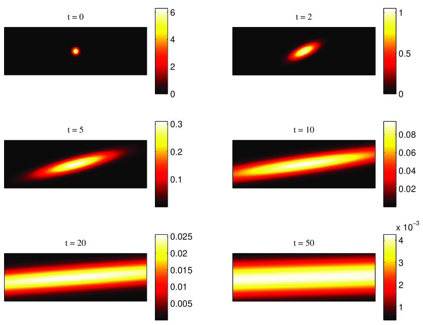
Figure 2: A patch of dye in a uniform shearing flow. The amplitude of the concentration field decreases algebraically with time as $t^{-2}$. The length of the filament increases as $t^{3/2}$, whilst its width increases as $t^{1/2}$.

2.4 Three Dimensions

In three dimensions, there are three basic forms for the matrix $\sigma$:

$$\sigma^{\text{(3a)}}=\begin{pmatrix}\lambda_{1}&0&0\\ 0&\lambda_{2}&0\\ 0&0&-\lambda_{1}-\lambda_{2}\end{pmatrix}\ \text{;}\quad\sigma^{\text{(3b)}}=\begin{pmatrix}0&0&0\\ U^{\prime}&0&0\\ 0&U^{\prime}&0\end{pmatrix}\ \text{;}\quad\sigma^{\text{(3c)}}=\begin{pmatrix}\lambda&0&0\\ U^{\prime}&\lambda&0\\ 0&0&-2\lambda\end{pmatrix},$$

with corresponding fundamental matrices

$$\mathcal{T}^{\text{(3a)}}=\begin{pmatrix}{\mathrm{e}}^{-\lambda_{1}t}&0&0\\ 0&{\mathrm{e}}^{-\lambda_{2}t}&0\\ 0&0&{\mathrm{e}}^{(\lambda_{1}+\lambda_{2})t}\end{pmatrix}\ \text{;}\quad\mathcal{T}^{\text{(3b)}}=\begin{pmatrix}0&0&0\\ -U^{\prime}t&0&0\\ \tfrac{1}{2}(U^{\prime}t)^{2}&-U^{\prime}t&0\end{pmatrix}\ \text{;}$$ (42)

$$\mathcal{T}^{\text{(3c)}}=\begin{pmatrix}{\mathrm{e}}^{-\lambda t}&0&0\\ -U^{\prime}t\,{\mathrm{e}}^{-\lambda t}&{\mathrm{e}}^{-\lambda t}&0\\ 0&0&{\mathrm{e}}^{2\lambda t}\end{pmatrix}.$$ (43)

We can assume without loss of generality that $\lambda_{1}\geq 0$, $\lambda_{1}\geq\lambda_{2}$, and $U^{\prime}>0$, but the sign of $\lambda_{2}$ and $\lambda$ is arbitrary; however, we must have $\lambda_{3}=-\lambda_{1}-\lambda_{2}\leq 0$. The case of greatest interest to us is (3a). The relevant ${\bm{k}}(t)$, corresponding to (18), is

$$\mathcal{T}^{(3a)}_{t}\cdot{\bm{k}}_{0}=\left({\mathrm{e}}^{-\lambda_{1}t}\,{k_{0}}_{1}\,,\,{\mathrm{e}}^{-\lambda_{2}t}\,{k_{0}}_{2}\,,\,{\mathrm{e}}^{\lvert\lambda_{3}\rvert t}\,{k_{0}}_{3}\right)\,,$$ (44)

which is used in (14) to give

$$\theta({\bm{x}},t)=\int\hat{\theta}_{0}({\bm{k}}_{0})\,{\mathrm{e}}^{\mathrm{i}{\bm{k}}(t)\cdot{\bm{x}}}\exp\Bigl{\{}-\tfrac{1}{2}\kappa\Bigl{(}\lambda_{1}^{-1}\left(1-{\mathrm{e}}^{-2\lambda_{1}t}\right){k_{0}}_{1}^{2}\\ +\lambda_{2}^{-1}\left(1-{\mathrm{e}}^{-2\lambda_{2}t}\right){k_{0}}_{2}^{2}+\lvert\lambda_{3}\rvert^{-1}\left({\mathrm{e}}^{2\lvert\lambda_{3}\rvert t}-1\right){k_{0}}_{3}^{2}\Bigr{)}\Bigr{\}}\,{\mathrm{d}}^{3}k_{0}\,.$$ (45)

What happens next depends on the sign of $\lambda_{2}$: the question is whether ${\mathrm{e}}^{-2\lambda_{2}t}$ grows or decays for $t\gg\lvert\lambda_{2}\rvert^{-1}$. If $\lambda_{2}>0$, then we have

$$\theta({\bm{x}},t)\simeq\int\hat{\theta}_{0}({\bm{k}}_{0})\,{\mathrm{e}}^{\mathrm{i}{\bm{k}}(t)\cdot{\bm{x}}}\exp\Bigl{\{}-\tfrac{1}{2}\kappa\Bigl{(}\lambda_{1}^{-1}{k_{0}}_{1}^{2}\\ +\lambda_{2}^{-1}{k_{0}}_{2}^{2}+\lvert\lambda_{3}\rvert^{-1}\,{\mathrm{e}}^{2\lvert\lambda_{3}\rvert t}\,{k_{0}}_{3}^{2}\Bigr{)}\Bigr{\}}\,{\mathrm{d}}^{3}k_{0}\,,$$ (46)

whilst for $\lambda_{2}<0$

$$\theta({\bm{x}},t)\simeq\int\hat{\theta}_{0}({\bm{k}}_{0})\,{\mathrm{e}}^{\mathrm{i}{\bm{k}}(t)\cdot{\bm{x}}}\exp\Bigl{\{}-\tfrac{1}{2}\kappa\Bigl{(}\lambda_{1}^{-1}{k_{0}}_{1}^{2}\\ +\lvert\lambda_{2}\rvert^{-1}{\mathrm{e}}^{2\lvert\lambda_{2}\rvert t}{k_{0}}_{2}^{2}+\lvert\lambda_{3}\rvert^{-1}\,{\mathrm{e}}^{2\lvert\lambda_{3}\rvert t}{k_{0}}_{3}^{2}\Bigr{)}\Bigr{\}}\,{\mathrm{d}}^{3}k_{0}\,.$$ (47)

Both approximations are valid when $t\gg\max(\lambda_{1}^{-1}\,,\,\lvert\lambda_{2}\rvert^{-1})$. For $\lambda_{2}=0$ the situation is similar to the two-dimensional case (2a):

$$\theta({\bm{x}},t)\simeq\int\hat{\theta}_{0}({\bm{k}}_{0})\,{\mathrm{e}}^{\mathrm{i}{\bm{k}}(t)\cdot{\bm{x}}}\exp\Bigl{\{}-\frac{\kappa}{2\lambda_{1}}\Bigl{(}{k_{0}}_{1}^{2}+{\mathrm{e}}^{2\lambda_{1}t}{k_{0}}_{3}^{2}\Bigr{)}\Bigr{\}}\,{\mathrm{d}}^{3}k_{0}\,,$$

valid when $t\gg\lambda_{1}^{-1}$.

The rest of the calculation is very similar to the two-dimensional case (2a), in going from (24) to (32). In both (46) and (47) the $x_{3}$ direction is stabilised, that is we need to blow up the ${k_{0}}_{3}$ integral to remove the time dependence from the exponential, and find that the integral is dominated by ${k_{0}}_{3}\simeq 0$. The $x_{2}$ direction is also stabilised in (47), so we can set ${k_{0}}_{2}\simeq 0$. We thus find for $\lambda_{2}\geq 0$,

$$\theta({\bm{x}},t)\simeq{\mathrm{e}}^{-\lvert\lambda_{3}\rvert t}\,G\bigl{(}x_{3};\ell_{3}\bigr{)}\int\theta_{0}({\mathrm{e}}^{-\lambda_{1}t}x_{1},{\mathrm{e}}^{-\lambda_{2}t}x_{2},\tilde{}x_{3})\,{\mathrm{d}}\tilde{}x_{3}\,,$$ (48)

and for $\lambda_{2}<0$,

$$\theta({\bm{x}},t)\simeq{\mathrm{e}}^{-(\lvert\lambda_{2}\rvert+\lvert\lambda_{3}\rvert)t}\,G\bigl{(}x_{2};\ell_{2}\bigr{)}\,G\bigl{(}x_{3};\ell_{3}\bigr{)}\int\theta_{0}({\mathrm{e}}^{-\lambda_{1}t}x_{1},\tilde{}x_{2},\tilde{}x_{3})\,{\mathrm{d}}\tilde{}x_{2}\,{\mathrm{d}}\tilde{}x_{3}\,,$$ (49)

where $\ell_{i}\mathrel{\raisebox{0.29707pt}{:}\!\!=}\sqrt{\kappa/\lvert\lambda_{i}\rvert}$. Contracting directions have their spatial dependence given by a time-independent Gaussian, with an overall exponential decay; stretching directions do just that: they stretch the initial distribution, with no diffusive effect. Solutions of the form (48) are called pancakes, and those of the form (49) are called ropes or tubes.

There is another way of thinking about the asymptotic forms (32), (48), and (49) Balkovsky1999 : contracting directions are stabilised near some constant width $\ell_{j}$, and expanding directions lead to exponential growth of the width of an initial distribution along the direction. Thus, the volume of the initial distribution grows exponentially at a rate given by the sum of $\lambda_{i}$’s associated with stretching directions, but the total amount of $\theta$ remains fixed (the mean is conserved). Hence, the concentration at a point should decay inversely proportional to the volume, which is exactly what (32), (48), and (49) predict.

3 Random Strain Models

In Section 2 we analysed the deformation of a patch of concentration field (a ‘blob’) in a linear velocity field. Though this is interesting in itself, it is a far cry from reality. We will now inch slightly closer to the real world by giving a random time dependence to our velocity field.

3.1 A Single Blob

Consider a single blob in a two-dimensional linear velocity field of the type we treated in Section 2.2 (case (2a)). Now assume the orientation and stretching rate $\lambda$ of the straining flow change randomly every time $\tau$. This situation is depicted schematically in Figure 3.

\psfrag{e1}{${\mathrm{e}}^{-\lambda^{(1)}\tau}$}\psfrag{e2}{${\mathrm{e}}^{-\lambda^{(2)}\tau}$}\psfrag{e3}{${\mathrm{e}}^{-\lambda^{(3)}\tau}$}\psfrag{e4}{${\mathrm{e}}^{-\lambda^{(4)}\tau}$}\psfrag{e5}{${\mathrm{e}}^{-\lambda^{(5)}\tau}$}\psfrag{e6}{${\mathrm{e}}^{-\lambda^{(6)}\tau}$}\includegraphics[width=303.53267pt]{figs/randomstrainblob.eps}

Figure 3: A single blob being stretched for a time $\tau$ by successive random straining flows. The amplitude of the concentration field decays by $\exp(-\lambda^{(i)}\tau)$ at each period.

We assume that the time $\tau$ is much larger than a typical stretching rate $\lambda$, so that there is sufficient time for the blob to be deformed into its asymptotic form (32) at each period, which predicts that at each period the concentration field will decrease by a factor $\exp(-\lambda^{(i)}\tau)$, where $\lambda^{(i)}$ is the stretching rate at the $i$th period. The concentration field after $n$ periods will thus be proportional to the product of decay factors,

$$\theta \sim{\mathrm{e}}^{-\lambda^{(1)}\tau}{\mathrm{e}}^{-\lambda^{(2)}\tau}\cdots{\mathrm{e}}^{-\lambda^{(n)}\tau},$$

$$={\mathrm{e}}^{-(\lambda^{(1)}+\lambda^{(2)}+\cdots+\lambda^{(n)})\,\tau}.$$ (50)

We may rewrite this as

$$\theta\sim{\mathrm{e}}^{-\Lambda_{n}t},$$ (51)

where $t=n\tau$, and

$$\Lambda_{n}\mathrel{\raisebox{0.29707pt}{:}\!\!=}\frac{1}{n}\sum_{i=1}^{n}\lambda^{(i)}$$

is the ‘running’ mean value of the stretching rate at the $n$th period. As we let $n$ become large, how de we expect the concentration field to decay? We might expect that it would decay at the mean value $\bar{\lambda}$ of the stretching rates $\lambda^{(i)}$. This is not the case: the running mean (51) does not converge to the mean $\bar{\lambda}$. Rather, by the central limit theorem its expected value is $\bar{\lambda}$, but its fluctuations around that value are proportional to $1/\sqrt{t}$. These fluctuations have an impact on the decay rate of $\theta$.

The ensemble of variables $\lambda^{(i)}$ is known as a realisation. Now let us imagine performing our blob experiment several times, and averaging the resulting concentration fields: this is known as an ensemble average over realisations. Ensemble-averaging smooths out fluctuations present in each given realisation. We may then replace the running mean $\Lambda_{n}$ by a sample-space variable $\Lambda$, together with its probability distribution $P(\Lambda,t)$. The mean (expected value) of the $\alpha$th power of the concentration field is then proportional to

$$\overline{\theta^{\alpha}}\sim\int_{0}^{\infty}{\mathrm{e}}^{-\alpha\Lambda t}\,P(\Lambda,t)\,{\mathrm{d}}\Lambda\,.$$ (52)

The overbar denotes the expected value. The factor ${\mathrm{e}}^{-\alpha\Lambda t}$ gives the amplitude of $\theta^{\alpha}$ given that the mean stretching rate at time $t$ is $\Lambda$, and $P(\Lambda,t)$ measures the probability of that value of $\Lambda$ occuring at time $t$.

The form of the probability distribution function (PDF) $P(\Lambda,t)$ is given by the central limit theorem:

$$P(\Lambda,t)\simeq G\bigl{(}\Lambda-\bar{\Lambda};\sqrt{\beta/t}\bigr{)},$$ (53)

that is, a Gaussian distribution (31) with mean $\bar{\Lambda}$ and standard deviation $\sqrt{\beta/t}$. The quantity $\beta$ is a measure of the nonuniformity (or fluctuations) of stretching in the flow, both spatially and temporally. The decrease of the standard deviation $\sqrt{\beta/t}$ with time reflects the convergence of the average stretching rate to the Lyapunov exponent $\bar{\Lambda}$. I will say more about $\beta$ in Section 4.1, when we look at a practical example.

Actually, the central limit theorem only applies to values of $\Lambda$ that do not deviate too much from the mean. The theorem understimates the probability of rare events; a more general form of the PDF of $\Lambda$ comes from large deviation theory Ellis ; ShwartzWeiss ,

$$P(\Lambda,t)\simeq\sqrt{\frac{t\,\mathcal{S}^{\prime\prime}(0)}{2\pi}}\,{\mathrm{e}}^{-t\mathcal{S}(\Lambda-\bar{\Lambda})}.$$ (54)

(A derivation of (54) is given in Appendix 7.) The function $\mathcal{S}(x)$ is known as the rate function, the entropy function, or the Cramér function, depending on the context (that is, which literature one is reading). It is a time-independent convex function with a minimum value of $0$ at $0$: $\mathcal{S}(0)=\mathcal{S}^{\prime}(0)=0$. If $\Lambda$ is near the mean, we have

$$\mathcal{S}(\Lambda-\bar{\Lambda})\simeq\tfrac{1}{2}\,\mathcal{S}^{\prime\prime}(0)(\Lambda-\bar{\Lambda})^{2},$$ (55)

which recovers the Gaussian result (53) with $\beta=1/\mathcal{S}^{\prime\prime}(0)$. Both (53) and (54) are only valid for large $t$ (which in our case means $t\gg\tau$, or equivalently $n\gg 1$).

We can now evaluate the integral (52) with the PDF (54),

$$\overline{\theta^{\alpha}}\sim\int_{0}^{\infty}{\mathrm{e}}^{-tH(\Lambda)}\,\,{\mathrm{d}}\Lambda\sim{\mathrm{e}}^{-\gamma_{\alpha}t}\,,$$ (56)

where we have omitted the nonexponential prefactors, and defined

$$H(\Lambda)\mathrel{\raisebox{0.29707pt}{:}\!\!=}\alpha\Lambda+\mathcal{S}(\Lambda-\bar{\Lambda}).$$

Since $t$ is large, the integral is dominated by the minimum value of $H(\Lambda)$: this is the perfect setting for the well-known saddle-point approximation. The minimum occurs at $\Lambda_{\mathrm{sp}}$ where $H^{\prime}(\Lambda_{\mathrm{sp}})=\alpha+\mathcal{S}^{\prime}(\Lambda_{\mathrm{sp}}-\bar{\Lambda})=0$, and is unique because $\mathcal{S}$ is convex and has a unique minimum. The decay rate is then given by

$$\gamma_{\alpha}=H(\Lambda_{\mathrm{sp}}),\quad\text{with\quad}H^{\prime}(\Lambda_{\mathrm{sp}})=0.$$ (57)

There’s a caveat to this: for $\alpha$ large enough the saddle point $\Lambda_{\mathrm{sp}}$ is negative. This is not possible: the stretching rates are defined to be nonnegative (the integral (56) involves only nonnegative $\Lambda$). Hence, the best we can do is to choose $\Lambda_{\mathrm{sp}}=0$—the integral (56) is dominated by realisations with no stretching. Thus, in that case $\gamma_{\alpha}=H(0)$, or

$$\gamma_{\alpha}=\mathcal{S}(-\bar{\Lambda}).$$ (58)

We re-emphasise: for small enough $\alpha$, the saddle point is positive and the decay rate is given by (57). Beyond that, we must choose zero as the saddle point and the decay rate is given by (58). To find the critical value $\alpha_{\mathrm{crit}}$ where we pass from (57) to (58), observe that this happens as the saddle point nears zero. Thus, we may solve our saddle point equation $H^{\prime}(\Lambda_{\mathrm{sp}})=0$ by Taylor expansion,

$$H^{\prime}(\Lambda_{\mathrm{sp}})\simeq\alpha_{\mathrm{crit}}+\mathcal{S}^{\prime}(-\bar{\Lambda})+\Lambda_{\mathrm{sp}}\,\mathcal{S}^{\prime\prime}(-\bar{\Lambda})=0.$$ (59)

But the saddle point will not be small unless the first terms cancel in (59), that is $\alpha_{\mathrm{crit}}=-\mathcal{S}^{\prime}(-\bar{\Lambda})$. We may thus recapitulate the result for the decay rate,

$$\gamma_{\alpha}=\begin{cases}\alpha\Lambda_{\mathrm{sp}}+\mathcal{S}(\Lambda_{\mathrm{sp}}-\bar{\Lambda}),\qquad&\alpha<-\mathcal{S}^{\prime}(-\bar{\Lambda});\\[6.0pt] \mathcal{S}(-\bar{\Lambda}),\qquad&\alpha\geq-\mathcal{S}^{\prime}(-\bar{\Lambda}).\end{cases}$$ (60)

Clearly $\gamma_{\alpha}$ is continous, and it can be easily shown that $d\gamma_{\alpha}/d\alpha$ is also continuous.

As an illustration, we use the Gaussian approximation (55) for the Cramér function, with $\beta=1/\mathcal{S}^{\prime\prime}(0)$. The critical $\alpha$ is $\alpha_{\mathrm{crit}}=-\mathcal{S}^{\prime}(-\bar{\Lambda})=\bar{\Lambda}/\beta$. The saddle point is positive for $\alpha<\bar{\Lambda}/\beta$, so from (60) we get

$$\gamma_{\alpha}=\begin{cases}\alpha\left(\bar{\Lambda}-\tfrac{1}{2}\,\alpha\beta\right),\qquad&\alpha<\bar{\Lambda}/\beta;\\[6.0pt] \bar{\Lambda}^{2}/2\beta,\qquad&\alpha\geq\bar{\Lambda}/\beta.\end{cases}$$ (61)

This is plotted in Figure 4.

\psfrag{alpha}{\hskip 10.00002pt\raisebox{-3.00003pt}{$\alpha$}}\psfrag{alphac}{\raisebox{1.99997pt}{$\alpha_{\mathrm{crit}}$}}\psfrag{gamma}{\hskip 8.00003pt\raisebox{3.99994pt}{$\gamma_{\alpha}$}}\includegraphics[width=346.89731pt]{figs/gammablob.eps}

Figure 4: Decay rate (61) for the concentration of a blob in a Gaussian random stretching flow (solid curve). The dashed line is for a fixed, nonrandom flow as in Section 2.2. Here $\bar{\Lambda}=1$, $\beta=1/4$, so $\alpha_{\mathrm{crit}}=\bar{\Lambda}/\beta=4$.

Notice that the solid curve (for a random flow) lies below the dashed line (for a nonrandom flow). This is a general result: if $f(x)$ is a convex function and $x$ a random variable, Jensen’s inequality says that

$$\overline{f(x)}\geq f(\overline{x}).$$ (62)

Now, ${\mathrm{e}}^{-\alpha t\Lambda}$ is a convex funtion of $\Lambda$, so we have

$$\overline{{\mathrm{e}}^{-\alpha t\Lambda}}\geq{\mathrm{e}}^{-\alpha t\overline{\Lambda}},$$

which means that the rate of decay satisfies

$$\gamma_{\alpha}\leq\alpha\,\bar{\Lambda},$$

which is exactly what is seen in Figure 4. Thus, fluctuations in $\Lambda$ inevitably lead to a slower decay rate $\gamma_{\alpha}$.

Stronger fluctuations also means that the decay rate $\gamma_{\alpha}$ saturates more quickly with $\alpha$. Clearly, in the absence of fluctuations we recover the nonrandom result: $\bar{\Lambda}/\beta$ is infinite and only the $\alpha<\bar{\Lambda}/\beta$ case is needed in Eq. (61). If there are lots of fluctuations, $\bar{\Lambda}/\beta$ is small, and there is a greater probability of obtianing a realisation with no stretching. For large enough fluctuations this exponentially-decreasing probability dominates, and we obtain the second case in (60).

3.2 Many Blobs

In Section 3.1 we considered the evolution of the concentration of a single blob of concentration in a random straining field. Now we turn our attention to a large number of blobs, homogeneously and isotropically distributed, with random concentrations. We assume that the mean concentration over all the blobs is zero. A simplified view of this initial situation is depicted in Figure 5(a), with shades of gray indicating different concentrations.

\psfrag{(a)}{(a)}\psfrag{(b)}{(b)}\psfrag{(c)}{(c)}\psfrag{(d)}{(d)}\includegraphics[width=346.89731pt]{figs/overlapblobs.eps}

Figure 5: (a) An initial distribution of blobs with random concentrations (b) are stretched by a constant strain (c) until they reach the diffusive limit in the contracting direction and begin to overlap. (d) Finally, they combine into one very long blob with the average concentration of all the blobs.

If we now apply a uniform straining flow of the type (2a) (see Section 2.2), the blobs are all stretched horizontally (the $x_{1}$ direction) and contracted in the vertical ($x_{2}$) direction, as shown in Figure 5(b). They are pressed together in the $x_{2}$ direction until diffusion becomes important (Figure 5(c)). The effect of diffusion is to homogenise the concentration field until it reaches a value which is the average of the concentration of the individual blobs. This is depicted by the long gray blob in Figure 5(d), which will itself keep contracting until it reaches the diffusive length $\ell$.

Of course, here the initial concentration field $\theta_{0}$ represents the concentration of all the homogeneously-distributed blobs together, so it does not decay at infinity: we must thus use Eq. (30) rather than (32). The summing (and hence averaging) over blobs is manifest in Eq. (30), which contains an integral over the initial distribution $\theta_{0}$ in the $x_{2}$ direction, windowed by a Gaussian.

In practice, this implies that the expected value of the concentration at a point ${\bm{x}}$ on the gray filament is given by

$$\left\langle\theta({\bm{x}},t)\right\rangle_{\mathrm{blobs}}\sim{\mathrm{e}}^{-\Lambda t}\sum_{i}^{N}\overline{\theta_{0}^{(i)}}\longrightarrow 0\,,$$ (63)

where $\theta_{0}^{(i)}$ is the initial concentration of the $i$th blob, and $\left\langle\cdot\right\rangle_{\mathrm{blobs}}$ denotes the expected value of the sum over the overlapping blobs at point ${\bm{x}}$ (not the same as spatial integration $\left\langle\cdot\right\rangle$). We assume that $N\gg 1$ blobs have overlapped. Equation (63) gives the concentration at a point, summed over $N$ overlapping blobs. Of course, Eq. (63) converges to zero for large $N$, because the blobs average out. Not so for the fluctuations at that point: by the central limit theorem, we have

$$\left\langle\theta^{2}({\bm{x}},t)\right\rangle_{\mathrm{blobs}}\sim{\mathrm{e}}^{-2\Lambda t}\sum_{i}^{N}\overline{{\theta_{0}^{(i)}}^{2}}=N{\mathrm{e}}^{-2\Lambda t}\,\,\overline{\theta_{0}^{2}}\,,$$ (64)

since the initial blobs have identical distributions. The blob-summed fluctuation amplitude $\left\langle\theta^{2}\right\rangle_{\mathrm{blobs}}$ is thus proportional to the number $N$ of overlapping blobs. But the number of overlapping blobs is proportional to ${\mathrm{e}}^{\Lambda t}$: as time increases more and more blobs converge to a given ${\bm{x}}$ in the contracting direction and overlap diffusively (this can be seen in Eq. (30): the width of the windowing region grows as ${\mathrm{e}}^{\lambda t}$). Assuming the variance of $\theta_{0}^{(i)}$ is finite, we conclude from (64) that

$$\left\langle\theta^{2}({\bm{x}},t)\right\rangle_{\mathrm{blobs}}^{1/2}\sim{\mathrm{e}}^{-\Lambda t/2}\,.$$ (65)

Compare this to (51) for the single-blob case: the overlap between blobs has led to an extra square root. Thus, the ensemble averages $\overline{\left\langle\theta^{2}({\bm{x}},t)\right\rangle^{\alpha}}_{\!\!\!\mathrm{blobs}}$ for the overlapping blobs are computed exactly as in Section 3.1, resulting in (60). Because of the assumption of homogeneity, the point-average is the same as the average over the whole domain (see Section 4 for more on this), and we have

$$\left\langle\theta^{2}\right\rangle^{\alpha}=\overline{\left\langle\theta^{2}({\bm{x}},t)\right\rangle^{\alpha}}_{\!\!\!\mathrm{blobs}}\sim{\mathrm{e}}^{-\gamma_{\alpha}t}\,,$$ (66)

with $\gamma_{\alpha}$ given by (60). (In (66) the angle brackets denote spatial averaging, not spatial integration, because the total variance is infinite in this case.)

3.3 Three Dimensions

In three dimensions, we will only treat Case (3a) (a purely straining flow) of Section 2.4. For $\lambda_{2}<0$, where the asymptotic concentration is given by (49) (ropes), the situation is basically identical to the 2D case of Sections 3.1–3.2: the statistics of the stretching direction $\lambda_{1}$ determine $\gamma_{\alpha}$ from (60). The contracting directions $x_{2}$ and $x_{3}$ are stabilised by diffusion.

For $\lambda_{2}\geq 0$, the asymptotic concentration is given by (48) (pancakes). We have two fluctuating quantities to worry about ($\lambda_{1}$ and $\lambda_{2}$). But since the decay rate in (48) only depends on $\lambda_{3}$, we can instead focus on its fluctuations only. For a single blob, the average (52) is then replaced by

$$\overline{\theta^{\alpha}}\sim\int_{0}^{\infty}{\mathrm{e}}^{-\alpha\lvert\Lambda_{3}\rvert t}\,P_{3}(\lvert\Lambda_{3}\rvert,t)\,{\mathrm{d}}\lvert\Lambda_{3}\rvert\sim{\mathrm{e}}^{-\gamma_{\alpha}t}\,,$$ (67)

where of course $\Lambda_{3}$ is the average of $\lambda_{3}$. This PDF achieves a distribution of the large-deviation form (54). The analysis thus follows exactly as in Sections 3.1 and 3.2, except the Cramér function for $\lvert\Lambda_{3}\rvert$ must be used.

4 Practical Considerations

One may rightly wonder if the blobs in a random uniform straining flow depicted in Section 3 bear any resemblance to reality. The single-blob scenario doesn’t, but the many-blobs scenario has a fighting chance, as we will try to justify here. There are two important considerations: where does the ensemble-averaging come from, and what are the stretching rates given by?

The decay rate (60) depends crucially on ensemble-averaging: with that averaging the decay rate fluctuates wildly for a given realisation. At the end of Section 3.2 we assumed that homogeneity allowed us to generalise from the average at a point to the average over the whole domain. But the average over the whole domain can actually do a lot more for us: it can provide the ensemble of blobs that we need for averaging! Thus, we can forget about speaking of realisations as if we were running many parallel experiments, and instead speak of the moments of the concentration field as given by an average over randomly-distributed blobs. The decay rate will then be naturally smoothed-out over blobs experiencing different stretching histories. The saturation of the decay rate with $\alpha$ in Eq. (60) is due to $\overline{\theta^{2\alpha}}$ being dominated by the fraction of blobs that have experienced no stretching.

What about the stretching rates $\lambda$? Luckily, it is not them but their time-average $\Lambda$ that matters. If we imagine following a blob as it moves through the flow, we can see that this time-averaged stretching rate is nothing but the finite-time Lyapunov exponent associated with this blob and its particular initial condition. A given blob will be constantly reoriented as it moves along in the flow, so its finite-time Lyapunov exponent is not just the average of the stretching rates (in fact, it must be strictly less than this average). But in a chaotic system we are guaranteed that, on average, these reorientations do not lead to a vanishing (infinite-time) Lyapunov exponent. This is guaranteed by the celebrated Oseledec multiplicative theorem for random matrices Oseledec1968 . We may thus use for $P(\Lambda,t)$ the distribution of finite-time Lyapunov exponents, which is well-known to have the large-deviation form (54) Ott .

The result of these considerations is the local theory of passive scalar decay. It is called local because of the reliance of such a local concept as the finite-time Lyapunov exponents, which come from a linearisation near fluid element trajectories. In Section 4.1 we discuss a specific example. We postpone a discussion of the validity of the local theory until Section 4.2, but for now we point out that it is known to be exact at least in some simple model flows Fouxon1998 ; Balkovsky1999 .

The derivation presented in this Section was based on the work of Balkovsky and Fouxon Balkovsky1999 , who used a slightly more rigorous approach. Son Son1999 also obtained the decay rate (60) using path-integral methods. Earlier, Antonsen et al. Antonsen1996 derived the decay rate for the second moment $\left\langle\theta^{2}\right\rangle$ in terms of the Cramér function, using a different (and not quite equivalent) approach, though they did not allow for the second case in (60).

4.1 An Example: Flow in a Microchannel

We illustrate how to compute the decay rates $\gamma_{\alpha}$ with a practical problem. Specifically, we will use a three-dimensional model of a microchannel. The system is shown in Figure 6.

\psfrag{x}[c][c]{\Large{$x$}}\psfrag{y}[c][c]{\Large{$y$}}\psfrag{z}[c][c]{\Large{$z$}}\psfrag{0}[c][c]{\Large{$0$}}\psfrag{h}[c][c]{\Large{$h$}}\psfrag{-l/2}[c][c]{\large{$-\frac{\ell}{2}$}}\psfrag{l/2}[c][c]{\large{$\frac{\ell}{2}$}}\includegraphics[width=303.53267pt]{figs/herring3D.eps}

Figure 6: Microchannel with a periodic patterned electro-osmotic potential at the bottom. The arrows indicate the direction of fluid motion at the bottom. The width of the channel is about $100\,\mu$m and its height $10$–$50\,\mu$m, and the period of the pattern is $L$. A typical mean fluid velocity is $10^{2}$–$10^{3}\,\mu\mathrm{m}/\mathrm{s}$.

It consists of a narrow channel, roughly $100\,\mu\mathrm{m}$ wide and slightly shallower. These types of channel are widely used in microfluidics applications (“lab-on-a-chip”), and often one wants to achieve good mixing in the lateral cross-section of the channel. This is difficult, since the Reynolds number of the flow varies between $0.1$ and $100$—far from turbulent. Clever techniques have to be used to induce chaotic motion of the fluid particle trajectories in order to enhance mixing. Stroock et al. Stroock2002 used patterned grooves at the bottom of the channel to induce vortical motions, and found that the mixing efficiency was dramatically increased. Here we use a variation on this where the bottom is pattern with an electro-osmotic coating, which induces fluid motion near the wall HongIMECE2003 . The effect of the electro-osmotic coating is well-approximated by a moving wall boundary condition. The pattern is chosen in a so-called herringbone pattern to maximise the mixing efficiency (though not in a staggered herringbone, which is even better but is more difficult to model). Rather than solving the full equations numerically, we adopt here an analytical model based on Stokes flow in a shallow layer EwartThiffeaultPreprint . The longitudinal ($x$) direction is taken to be periodic. The flow is steady, but because it is three-dimensional it can still exhibit chaos.

Figure 7 shows two Poincaré sections for the flow. These are taken at two constant $x$ planes, one at $x=0$ and the other at the mipoint of the $x$-periodic pattern. The two colours represent two trajectories that have periodically punctured those planes many times over.

\psfrag{y}[c][c]{\raisebox{-6.45831pt}{$y$}}\psfrag{z}[c][c]{\raisebox{3.87495pt}{$z$}}\psfrag{Section a3b5, a=0, U0=5, Lx0.000}[c][c]{Section at $x=0$}\psfrag{Section a3b5, a=0, U0=5, Lx0.500}[c][c]{Section at midpoint $x=L/2$}\includegraphics[width=303.53267pt]{figs/sect_a3b5_a=0_U0=5_Lx0.000.eps}

\psfrag{y}[c][c]{\raisebox{-6.45831pt}{$y$}}\psfrag{z}[c][c]{\raisebox{3.87495pt}{$z$}}\psfrag{Section a3b5, a=0, U0=5, Lx0.000}[c][c]{Section at $x=0$}\psfrag{Section a3b5, a=0, U0=5, Lx0.500}[c][c]{Section at midpoint $x=L/2$}\includegraphics[width=303.53267pt]{figs/sect_a3b5_a=0_U0=5_Lx0.500.eps}

Figure 7: Poincaré sections for the microchannel. The red and blue dots represent the same trajectory periodically puncturing two vertical planes many times over (blue if in the same direction as the flow, red otherwise). The green and yellow dots show two trajectories in regular, nonmixing regions.

It is clear from the Figures that the flow contains large chaotic regions, as well as smaller regular regions (known as islands). We focus here on the chaotic regions.

Now that we have established (or at least strongly suspect) the existence of chaotic regions, we can compute the distribution of finite-time Lyapunov exponents. There are many ways of doing this: because we are not interested in exetremely long times, the most direct route may be used. We have an analytical form for the velocity field, so the velocity gradient matrix is easily computed. This allows us to linearise about trajectories in the standard manner Eckmann1985 ; Ott . Each trajectory will thus have a finite-time Lyapunov exponent associated with it, which shows the tendency of infinitesimally close trajectories to diverge exponentially. This is then repeated over many different trajectories within the same chaotic region, and a histogram is made of the finite-time Lyapunov exponents. This histogram changes with time, as shown in Figure 8.

\psfrag{PDF of FTLEs}{\raisebox{5.0pt}{\tiny PDF of FTLEs}}\psfrag{FTLEs}{\hskip 10.00002pt\raisebox{-5.0pt}{\tiny FTLEs}}\psfrag{U0=5 with 20 modes}{\raisebox{2.5pt}{\hskip 5.0pt$t=19\,\mathrm{s}$}}\includegraphics[width=346.89731pt]{figs/Lyapdist_alpha=3_beta=5_t=18.9_U0=5_N=20.eps}

\psfrag{PDF of FTLEs}{\raisebox{5.0pt}{\tiny PDF of FTLEs}}\psfrag{FTLEs}{\hskip 10.00002pt\raisebox{-5.0pt}{\tiny FTLEs}}\psfrag{U0=5 with 20 modes}{\raisebox{2.5pt}{\hskip 5.0pt$t=38\,\mathrm{s}$}}\includegraphics[width=346.89731pt]{figs/Lyapdist_alpha=3_beta=5_t=37.8_U0=5_N=20.eps}

\psfrag{PDF of FTLEs}{\raisebox{5.0pt}{\tiny PDF of FTLEs}}\psfrag{FTLEs}{\hskip 10.00002pt\raisebox{-5.0pt}{\tiny FTLEs}}\psfrag{U0=5 with 20 modes}{\raisebox{2.5pt}{\hskip 5.0pt$t=57\,\mathrm{s}$}}\includegraphics[width=346.89731pt]{figs/Lyapdist_alpha=3_beta=5_t=56.7_U0=5_N=20.eps}

\psfrag{PDF of FTLEs}{\raisebox{5.0pt}{\tiny PDF of FTLEs}}\psfrag{FTLEs}{\hskip 10.00002pt\raisebox{-5.0pt}{\tiny FTLEs}}\psfrag{U0=5 with 20 modes}{\raisebox{2.5pt}{\hskip 5.0pt$t=76\,\mathrm{s}$}}\includegraphics[width=346.89731pt]{figs/Lyapdist_alpha=3_beta=5_t=75.6_U0=5_N=20.eps}

Figure 8: Evolution of the distribution of finite-time Lyapunov exponents for the microchannel. The average crossing time for particles in the channel is $L/U$.

For these relatively early times, it changes dramatically and does not show a self-similar form.

The evolution of the mean and standard deviation of the distribution is shown in Figure 9. The mean is converging to a constant $\bar{\Lambda}\simeq 0.116$, and the standard deviation is decreasing as $\sqrt{\beta/t}$, with $\beta\simeq 0.168$.

\psfrag{Mean}{\raisebox{5.0pt}{Mean}}\psfrag{Time}{\raisebox{-6.00006pt}{$t$}}\psfrag{Mean of 1st Lyapunov Exponent vs Time}{}\includegraphics[width=190.79385pt]{figs/Lyap_1_mean_vs_t.eps}

\psfrag{Standard Deviation}{\raisebox{5.0pt}{Standard Deviation}}\psfrag{1/sqrt(Time)}{\raisebox{-6.00006pt}{$1/\sqrt{t}$}}\psfrag{Standard Deviation of Lyapunov Exponent vs 1/sqrt(Time)}{}\includegraphics[width=190.79385pt]{figs/Lyap_SD_vs_1_sqrtt.eps}

Figure 9: (a) Evolution of the mean $\bar{\Lambda}$ of the distribution of Lyapunov exponents. The mean converges to $\bar{\Lambda}\simeq 0.116\,\,{\mathrm{s}}^{-1}$. (b) Standard deviation of the distribution of Lyapunov exponents versurs $1/\sqrt{t}$. The straight line represents $\sqrt{{\beta}/{t}}$, with $\beta\simeq 0.168\,\,{\mathrm{s}}^{-1}$.

(Both $\bar{\Lambda}$ and $\beta$ are fitted values, and arise from the complicated nonlinear nature of fluid particle trajectories—they cannot be predicted or calculated from first principles except in the simplest cases.) These facts taken together are strongly indicative that the distribution is converging to a Gaussian of the form (53). This is easily confirmed by plotting the PDFs at different times and rescaling the horizontal axis by $\sqrt{t}$, as shown in Figure 10.

\psfrag{Shifted Lyapunov Exponents with 20 Fourier Modes}{}\psfrag{$LyapunovExponent-Mean$ * sqrt$Time$}{\hskip 57.50008pt\raisebox{-5.0pt}{$\sqrt{t}\,(\Lambda-\bar{\Lambda})$}}\psfrag{Normalised PDF}{\raisebox{2.5pt}{Normalised PDF}}\includegraphics[width=303.53267pt]{figs/Lyap_sqrtt_t=201.6-504_U0=5_N=20.eps}

Figure 10: Rescaled distribution of finite-time Lyapunov exponents at different times. The dashed line is the Gaussian form (53), with parameters as in the caption for Figure 9.

Note that this case exhibits a particularly nice Gaussian form, which is not necessarily the norm for all chaotic flows.

Using the values for $\bar{\Lambda}$ and $\beta$ we just obtained, we can calculate the decay rates $\gamma_{\alpha}$ with the Gaussian approximation. The ratio $\bar{\Lambda}/\beta$ is $0.69$, so the change in character in (61) occurs at $\alpha\geq 0.69$. Since from (66) the decay of $\left\langle\theta^{2}\right\rangle^{\alpha}$ is given by $\gamma_{\alpha}$, this means that moments of order $2\alpha\geq 1.38$ will decay at the same rate. This includes the variance $\left\langle\theta^{2}\right\rangle$, so we have from (66)

$$\left\langle\theta^{2}\right\rangle\sim{\mathrm{e}}^{-\gamma_{1}t},\quad\text{with}\quad\gamma_{1}=\bar{\Lambda}^{2}/2\beta\simeq 0.040\,\,{\mathrm{s}}^{-1}.$$

The mixing time is thus $\gamma_{1}^{-1}\simeq 25$ seconds. This is about a factor of four improvement over the purely diffusive time for, say, DNA molecules ($\kappa\simeq 10^{-10}\,\,\mathrm{m^{2}\,s}^{-1}$). This is not spectacular, but can be greatly increased by staggering the herringbone pattern. The mixing time assuming the decay proceeds at the rate of the mean Lyapunov exponent $\bar{\Lambda}$ is roughly $9$ seconds, so that the fluctuations multiply this by a factor of three!

Of course, we do not know if this is actually a good estimate for the mixing time, since we haven’t directly solved the advection–diffusion equation numerically: this is prohibitive in a three-dimensional domain for such a small diffusivity. This is one of the advantages of the local theory: it is usually less expensive to compute the distribution of finite-time Lyapunov exponents than it is to solve the advection–diffusion equation equation directly. We will say more on the validity of the local theory in Section 4.2.

4.2 Limitations of the Local Theory

So is this local theory of mixing correct? Well, certainly not always, even in the Batchelor regime. There are many assumptions underlying the model, some of them difficult to verify. (Do blobs really undergo a series of stretching events as described here? Do correlations between these events matter?) My feeling is that sometimes it will, but most of the time it won’t. More experiments and numerical simulations are needed to get to the bottom of this. For a detailed discussion of possible problems with the local theory, see Fereday and Haynes Fereday2004 . They make a good case that the theory must break down for long times: the blobs discussed here meet the boundaries of the fluid domain and must begin to fold. The folding forces them to interact with themselves in a correlated fashion. We enter the regime of the strange eigenmode Pierrehumbert1994 , which has received a lot of attention lately Rothstein1999 ; Fereday2002 ; Sukhatme2002 ; Wonhas2002 ; Pikovsky2003 ; Thiffeault2003d ; Fereday2004 ; Liu2004 ; Thiffeault2004b ; Schekochihin2004 . Maybe we’ll hear more about that in ten years….

5 The Advection–Diffusion Equation in a Comoving Frame

We start from the advection–diffusion equation (1) and derive its form (8) for a linearised velocity field. We want to transform from the fixed spatial coordinates ${\bm{x}}$ to coordinates $\bm{r}$ measured from a reference fluid trajectory ${\bm{x}}_{0}(t)$. The coordinates $\bm{r}$ are not quite material (Lagrangian) coordinates, since we follow the trajectory of only one fluid element.

We thus let

$${\bm{x}}={\bm{x}}_{0}(t)+\bm{r},\qquad\frac{d{\bm{x}}_{0}(t)}{dt}={\bm{v}}({\bm{x}}_{0}(t),t),$$ (68)

and write the concentration field as

$$\theta({\bm{x}},t)=\tilde{\theta}(\bm{r},t).$$

The time derivative of $\theta$ can be written

$${\left.\frac{\partial}{\partial t}\right\rvert}_{{\bm{x}}}\theta({\bm{x}},t)={\left.\frac{\partial}{\partial t}\right\rvert}_{\bm{r}}\tilde{\theta}(\bm{r},t)+\nabla_{\bm{r}}\tilde{\theta}\cdot{\left.\frac{\partial\bm{r}}{\partial t}\right\lvert}_{{\bm{x}}},$$ (69)

where $\partial/\partial t\rvert_{{\bm{x}}}$ denotes a derivative with ${\bm{x}}$ held constant. Now from (68)

$${\left.\frac{\partial\bm{r}}{\partial t}\right\lvert}_{{\bm{x}}}=-\frac{d{\bm{x}}_{0}}{dt}=-{\bm{v}}({\bm{x}}_{0}(t),t).$$

Spatial derivatives are unchanged by (68): $\nabla_{{\bm{x}}}\theta=\nabla_{\bm{r}}\tilde{\theta}$. Hence, inserting (69) into (1), we find

$${\left.\frac{\partial}{\partial t}\right\rvert}_{\bm{r}}\tilde{\theta}+\{{\bm{v}}({\bm{x}}_{0}(t)+\bm{r},t)-{\bm{v}}({\bm{x}}_{0}(t),t)\}\cdot\nabla_{\bm{r}}\tilde{\theta}=\kappa\,\nabla^{2}_{\bm{r}}\tilde{\theta}\,.$$ (70)

We Taylor expand the velocity field in (70) to get

$${\left.\frac{\partial}{\partial t}\right\rvert}_{\bm{r}}\tilde{\theta}+\bm{r}\cdot\sigma(t)\cdot\nabla_{\bm{r}}\tilde{\theta}=\kappa\,\nabla^{2}_{\bm{r}}\tilde{\theta}\,,\qquad\sigma(t)\mathrel{\raisebox{0.29707pt}{:}\!\!=}\nabla{\bm{v}}({\bm{x}}_{0}(t),t),$$ (71)

where we neglected terms of order $\lvert\bm{r}\rvert^{2}$. This is only valid if the velocity field changes little over the region we consider (i.e., if it is smooth enough), which is true for large Schmidt number. Equation (71) is the same as (8), and tells us how to find $\sigma(t)$.

6 Volume Preservation

It is useful to know how to prove that a divergence-free vector field will lead to volume-preservation of a small blob of integrated trajectories. Mathematically, we want to go from (11) to (12). We start from the definition of the determinant of a $d$-dimensional matrix,

$$\det\mathcal{T}=\sum_{i_{1}\cdots i_{d}}\sum_{j_{1}\cdots j_{d}}\frac{1}{d!}\,\epsilon_{i_{1}\cdots i_{d}}\,\epsilon_{j_{1}\cdots j_{d}}\,\mathcal{T}_{i_{1}j_{1}}\cdots\mathcal{T}_{i_{d}j_{d}}$$ (72)

where we have dropped the ‘$t$’ subscript from $\mathcal{T}$ for this section, and $\epsilon$ is the fully-antisymmetric Levi-Civita symbol. Taking a time derivative of (72),

$$\partial_{t}\det\mathcal{T}=\sum_{i_{1}\cdots i_{d}}\sum_{j_{1}\cdots j_{d}}\frac{1}{(d-1)!}\,\epsilon_{i_{1}\cdots i_{d}}\,\epsilon_{j_{1}\cdots j_{d}}\,\partial_{t}\mathcal{T}_{i_{1}j_{1}}\cdots\mathcal{T}_{i_{d}j_{d}}$$ (73)

since the $d$ terms obtained after using the product rule for derivatives are the same. We use the equation of motion (11) for $\mathcal{T}$,

$$\partial_{t}\det\mathcal{T}=-\sum_{i_{1}\cdots i_{d}}\sum_{j_{1}\cdots j_{d}}\sum_{\ell}\frac{1}{(d-1)!}\,\epsilon_{i_{1}\cdots i_{d}}\,\epsilon_{j_{1}\cdots j_{d}}\,\sigma_{i_{1}\ell}\,\mathcal{T}_{\ell j_{1}}\,\mathcal{T}_{i_{2}j_{2}}\cdots\mathcal{T}_{i_{d}j_{d}}\,.$$

We rearrange the sums on the right,

$$\partial_{t}\det\mathcal{T}=-\sum_{i_{1},j_{1},\ell}\sigma_{i_{1}\ell}\,\mathcal{T}_{\ell j_{1}}\,\left(\sum_{i_{2}\cdots i_{d}}\sum_{j_{2}\cdots j_{d}}\frac{1}{(d-1)!}\,\epsilon_{i_{1}\cdots i_{d}}\,\epsilon_{j_{1}\cdots j_{d}}\,\mathcal{T}_{i_{2}j_{2}}\cdots\mathcal{T}_{i_{d}j_{d}}\right)$$

and recognise that, up to a factor of $\det\mathcal{T}$, the term in the parentheses is the cofactor representation of the inverse of $\mathcal{T}$:

$$\partial_{t}\det\mathcal{T}=-\sum_{i_{1},j_{1},\ell}\sigma_{i_{1}\ell}\,\mathcal{T}_{\ell j_{1}}\,(\mathcal{T}^{-1})_{j_{1}i_{1}}\,\det\mathcal{T}=-\sum_{i_{1},\ell}\sigma_{i_{1}\ell}\,\delta_{\ell i_{1}}\,\det\mathcal{T}$$

so that finally

$$\partial_{t}\det\mathcal{T}=-(\operatorname{Tr}\sigma)\,\det\mathcal{T}\,.$$

We conclude that if $\operatorname{Tr}\sigma=0$ then the determinant of $\mathcal{T}$ is constant. Since its initial condition is unity (from Eq. (11)), then it must remain so for all time.

7 Large Deviation Theory

In this Appendix we will justify the large-deviation form of the PDF, Eq. (54), assuming little prior knowledge of probability theory.

First, we define the characteristic function ${\mathrm{e}}^{-s(k)}$ of a random variable $x$ by

$${\mathrm{e}}^{-s(k)}=\int p(x)\,{\mathrm{e}}^{-\mathrm{i}\,kx}\,\,{\mathrm{d}}x\,,$$

that is, the characteristic function is simply the Fourier transform of the PDF of $x$. We have $s(0)=0$, $\bar{x}=-\mathrm{i}\,s^{\prime}(0)$, and $\overline{x^{2}}-{\bar{x}}^{2}=s^{\prime\prime}(0)$. Now define the random variable $X$ to be the mean of $n$ variables,

$$X_{n}=\frac{1}{n}\,\sum_{i=1}^{n}x_{i}$$

where the $x_{i}$ are independent and identically distributed with PDF $p(x_{i})=p(x)$. How do we find the PDF $P(X_{n})$ of $X_{n}$, in the limit where $n$ is large? First observe that (from here on we drop the subscript on $X_{n}$)

$$P(X)=\int p(x_{1})\cdots p(x_{n})\,\,\delta\left(\frac{x_{1}+\cdots+x_{n}}{n}-X\right)\!\,{\mathrm{d}}x_{1}\cdots\,{\mathrm{d}}x_{n}$$

since the joint PDF $p(x_{1},\ldots,x_{n})=p(x_{1})\cdots p(x_{n})$ by independence of the $x_{i}$. The characteristic function ${\mathrm{e}}^{-S(k)}$ for $P(X)$ is then

$${\mathrm{e}}^{-S(k)} =\int P(X)\,{\mathrm{e}}^{-\mathrm{i}kX}\,{\mathrm{d}}X$$

$$=\int p(x_{1})\cdots p(x_{n})\,\delta\!\left(\frac{x_{1}+\cdots+x_{n}}{n}-X\right)\!{\mathrm{e}}^{-\mathrm{i}kX}\,{\mathrm{d}}x_{1}\cdots\,{\mathrm{d}}x_{n}\,{\mathrm{d}}X$$

We do the $X$ integral, and then observe that we get a product of $n$ identical $x_{i}$ integrals, each of which is equal to ${\mathrm{e}}^{-s(k/n)}$:

$${\mathrm{e}}^{-S(k)}=\int p(x_{1})\cdots p(x_{n})\,\,{\mathrm{e}}^{-\mathrm{i}(k/n)(x_{1}+\cdots+x_{n})}\,{\mathrm{d}}x_{1}\cdots\,{\mathrm{d}}x_{n}={\mathrm{e}}^{-ns(k/n)}\,.$$

Thus the characteristic function for $X$ is the $n$th power of the characteristic function for $x$. We can invert the Fourier transform to find the PDF $P(X)$:

$$P(X)=\frac{1}{2\pi}\int{\mathrm{e}}^{-S(k)}\,{\mathrm{e}}^{\mathrm{i}\,kX}\,{\mathrm{d}}k=\frac{n}{2\pi}\int{\mathrm{e}}^{-n(s(K)-\mathrm{i}\,KX)}\,{\mathrm{d}}K$$ (74)

where $K=k/n$. We let

$$H(K,X)=s(K)-\mathrm{i}\,KX\,;$$

For large values of $n$ the integral in (74) is dominated by the stationary points $K_{\mathrm{sp}}(X)$ of $H(K,X)$ (saddle-point approximation):

$$K_{\mathrm{sp}}(X)\quad\text{such that}\quad\frac{\partial H}{\partial K}(K_{\mathrm{sp}},X)=s^{\prime}(K_{\mathrm{sp}})-\mathrm{i}\,X=0.$$ (75)

(I will often leave out the $X$ dependence of $K_{\mathrm{sp}}(X)$ to shorten the expressions.) In that case we can approximate the integrand in (74) using

$$H(K,X)=H(K_{\mathrm{sp}},X)+\tfrac{1}{2}\,s^{\prime\prime}(K_{\mathrm{sp}})(K-K_{\mathrm{sp}})^{2}+\mathcal{O}\!\left((K-K_{\mathrm{sp}})^{3}\right)$$

which allows us to do the integral explicitly:

$$P(X)=\sqrt{\frac{n}{2\pi\,s^{\prime\prime}(K_{\mathrm{sp}}(X))}}\,\,{\mathrm{e}}^{-nH(K_{\mathrm{sp}}(X),X)}$$ (76)

where $K_{\mathrm{sp}}(X)$ is given by (75). As a final step, let us calculate the mean of $X$ using this PDF:

$$\overline{X}=\int XP(X)\,{\mathrm{d}}X=\int X\sqrt{\frac{n}{2\pi\,s^{\prime\prime}(K_{\mathrm{sp}}(X))}}\,\,{\mathrm{e}}^{-nH(K_{\mathrm{sp}}(X),X)}\,{\mathrm{d}}X\,.$$ (77)

Again, for large $n$ we can use the saddle-point method to evaluate this integral. The important observation is that the saddle-point $X_{\mathrm{0}}$ of $H_{\mathrm{sp}}(K(X),X)$ satisfies

$$\frac{dH}{dX}(K_{\mathrm{sp}}(X_{\mathrm{0}}),X_{\mathrm{0}})=\frac{\partial H}{\partial K}(K_{\mathrm{sp}}(X_{\mathrm{0}}),X_{\mathrm{0}})\,\frac{dK_{\mathrm{sp}}}{dX}(X_{\mathrm{0}})-\mathrm{i}\,K_{\mathrm{sp}}(X_{\mathrm{0}})=0.$$

The $\partial H/\partial K$ term vanishes because it is evaluated at $K_{\mathrm{sp}}$; hence, $K_{\mathrm{sp}}(X_{\mathrm{0}})=0$, which implies $H(K_{\mathrm{sp}}(X_{\mathrm{0}}),X_{\mathrm{0}})=0$. Inserting this into the integral (77), we find $\overline{X}=X_{\mathrm{0}}$: the mean of $X$ and the minimum of $H$ coincide. This means that it makes sense to define

$$\mathcal{S}(X-\overline{X})\mathrel{\raisebox{0.29707pt}{:}\!\!=}H(K_{\mathrm{sp}}(X),X),\quad\text{with }\mathcal{S}(0)=0\text{ and }\mathcal{S}^{\prime}(0)=0,$$ (78)

which is the sought-after Cramér function. Note also that $\mathcal{S}^{\prime\prime}(X-\overline{X})=1/s^{\prime\prime}(K_{\mathrm{sp}}(X))$, and that for large $n$ the non-exponential coefficient in (76) can thus be approximated by evaluating it at the saddle-point $K_{\mathrm{sp}}(\overline{X})=0$, with $s^{\prime\prime}(0)=1/\mathcal{S}^{\prime\prime}(0)$. The final form of our large-deviation result is thus

$$P(X)=\sqrt{\frac{n\,\mathcal{S}^{\prime\prime}(0)}{2\pi}}\,\,{\mathrm{e}}^{-n\mathcal{S}(X-\overline{X})}$$ (79)

which is the same as Eq. (54).

As a simple example (treated in every textbook, see for example ShwartzWeiss ), consider a random variable $x$ with PDF

$$p(x)=(1-\varepsilon)\,\delta(x-x_{+})+\varepsilon\,\delta(x-x_{-}),$$ (80)

where $x_{+}>x_{-}$ are constants—this is a binomial distribution (or Bernoulli distribution in this case). If we take the mean $X$ of $n$ such variables, what is the PDF of $X$ for large $n$? First, we compute the characteristic function for $x$,

$${\mathrm{e}}^{-s(k)} =\int\left\{(1-\varepsilon)\,\delta(x-x_{+})+\varepsilon\,\delta(x-x_{-})\right\}{\mathrm{e}}^{-\mathrm{i}\,kx}\,{\mathrm{d}}x$$

$$=(1-\varepsilon)\,{\mathrm{e}}^{-\mathrm{i}\,kx_{+}}+\varepsilon\,{\mathrm{e}}^{-\mathrm{i}\,kx_{-}}\,.$$ (81)

We take the logarithm to obtain $s(k)$ and find $K_{\mathrm{sp}}(X)$ by solving the saddle-point equation (75),

$$\frac{\partial H}{\partial K}=s^{\prime}(K_{\mathrm{sp}})-\mathrm{i}\,X=0\quad\Longleftrightarrow\quad K_{\mathrm{sp}}(X)=\frac{1}{\mathrm{i}\Delta}\,\log\left(\frac{1-\varepsilon}{\varepsilon}\,\frac{x_{+}-X}{X-x_{-}}\right),$$

where $\Delta\mathrel{\raisebox{0.29707pt}{:}\!\!=}x_{+}-x_{-}$ and we restrict $x_{-}\leq X\leq x_{+}$. Inserting this into $H(K_{\mathrm{sp}}(X),X)$, we find from (78)

$$\mathcal{S}(X-\overline{X})=-\frac{X-x_{-}}{\Delta}\,\log\left(\frac{1-\varepsilon}{\varepsilon}\,\frac{x_{+}-X}{X-x_{-}}\right)+\log\left(\frac{x_{+}-X}{\varepsilon\Delta}\right).$$

It is easy to verify that, since $\overline{X}=(1-\varepsilon)x_{+}+\varepsilon\,x_{-}$, we have $\mathcal{S}(0)=\mathcal{S}^{\prime}(0)=0$ and $\overline{X^{2}}-{\overline{X}}^{2}=1/\mathcal{S}^{\prime\prime}(0)=\varepsilon(1-\varepsilon)\,\Delta^{2}$.

The binomial distribution (80) is a useful model of stretching of an infinitesimal line segment by a uniform incompressible straining flow in two dimensions, assuming the straining axes of the flow change direction randomly at regular intervals $\tau$. If we set $x_{\pm}=\pm\lambda\tau=\pm\beta$, where $\lambda$ is the strain rate, then $X$ is the averaged logarithm of the length $\ell$ of the segment, i.e. $\ell={\mathrm{e}}^{nX}$. Thus, the $m$th power of the length of the segment will on average grow as

$$\overline{\ell^{m}}=\overline{{\mathrm{e}}^{mnX}}={\mathrm{e}}^{-S(\mathrm{i}\,mn)}={\mathrm{e}}^{-ns(\mathrm{i}\,m)}=\left\{(1-\varepsilon)\,{\mathrm{e}}^{\beta m}+\varepsilon\,{\mathrm{e}}^{-\beta m}\right\}^{n}\,.$$ (82)

We know that $\overline{\ell^{-2}}$ must be constant in a 2D incompressible flow Falkovich2001 , so that the term in braces in (82) must be unity. We use this to solve for $\varepsilon$,

$$\varepsilon=(1+{\mathrm{e}}^{2\beta})^{-1},$$

which then allows us to use (82) to write the growth rate $\chi_{m}$ of line segments as

$$\chi_{m}=\frac{1}{\tau\,n}\log\overline{\ell^{m}}=\frac{1}{\tau}\log\left(\frac{\cosh(m+1)\beta}{\cosh\beta}\right)$$

The Lyapunov exponent, which is given by $d\chi_{m}/dm$ at $m=0$, has a value of $\lambda\tanh\beta$ for this flow: it is less than for a uniform straining flow because of the time taken for the segment to realign with the new straining axis when its direction changes.

References

- (1) G. K. Batchelor, “Small-scale variation of convected quantities like temperature in turbulent fluid: Part 1. General discussion and the case of small conductivity,” J. Fluid Mech. 5, 134 (1959).
- (2) R. H. Kraichnan, “Small-scale structure of a scalar field convected by turbulence,” Phys. Fluids 11, 945 (1968).
- (3) R. H. Kraichnan, “Convection of a passive scalar by a quasi-uniform random straining field,” J. Fluid Mech. 64, 737 (1974).
- (4) Y. B. Zeldovich, A. A. Ruzmaikin, S. A. Molchanov, and D. D. Sokoloff, “Kinematic dynamo problem in a linear velocity field,” J. Fluid Mech. 144, 1 (1984).
- (5) E. Ott and T. M. Antonsen, Jr., “Fractal measures of passively convected vector fields and scalar gradients in chaotic fluid flows,” Phys. Rev. A 39, 3660 (1989).
- (6) T. M. Antonsen, Jr. and E. Ott, “Multifractal power spectra of passive scalars convected by chaotic fluid flows,” Phys. Rev. A 44, 851 (1991).
- (7) T. M. Antonsen, Jr., Z. Fan, and E. Ott, “ spectrum of passive scalars in Lagrangian chaotic fluid flows,” Phys. Rev. Lett. 75, 1751 (1995).
- (8) T. M. Antonsen, Jr., Z. Fan, E. Ott, and E. Garcia-Lopez, “The role of chaotic orbits in the determination of power spectra,” Phys. Fluids 8, 3094 (1996).
- (9) B. I. Shraiman and E. D. Siggia, “Lagrangian path integrals and fluctuations in random flow,” Phys. Rev. E 49, 2912 (1994).
- (10) M. Chertkov, G. Falkovich, I. Kolokolov, and V. Lebedev, “Statistics of a passive scalar advected by a large-scale two-dimensional velocity field: Analytic solution,” Phys. Rev. E 51, 5609 (1995).
- (11) M. Chertkov, I. Kolokolov, and M. Vergassola, “Inverse cascade and intermittency of passive scalar in one-dimensional smooth flow,” Phys. Rev. E 56, 5483 (1997).
- (12) B. I. Shraiman and E. D. Siggia, “Scalar turbulence,” Nature 405, 639 (2000).
- (13) G. Falkovich, K. Gawȩdzki, and M. Vergassola, “Particles and fields in turbulence,” Rev. Mod. Phys. 73, 913 (2001).
- (14) J.-L. Thiffeault, “The strange eigenmode in Lagrangian coordinates,” Chaos 14, 531 (2004).
- (15) E. Balkovsky and A. Fouxon, “Universal long-time properties of Lagrangian statistics in the Batchelor regime and their application to the passive scalar problem,” Phys. Rev. E 60, 4164 (1999).
- (16) R. S. Ellis, Entropy, Large Deviations, and Statistical Mechanics (Springer-Verlag, New York, 1985).
- (17) A. Schwartz and A. Weiss, Large Deviations for Performance Analysis (Chapman & Hall, London, 1995).
- (18) V. I. Oseledec, “A multiplicative theorem: Lyapunov characteristic numbers for dynamical systems,” Trans. Moscow Math. Soc. 19, 197 (1968).
- (19) E. Ott, Chaos in Dynamical Systems (Cambridge University Press, Cambridge, U.K., 1994).
- (20) A. Fouxon, “Evolution of a scalar gradient’s probability density function in a random flow,” Phys. Rev. E 58, 4019 (1998).
- (21) D. T. Son, “Turbulent decay of a passive scalar in the Batchelor limit: Exact results from a quantum-mechanical approach,” Phys. Rev. E 59, R3811 (1999).
- (22) A. D. Stroock, S. K. W. Dertinger, A. Ajdari, I. Mezić, H. A. Stone, and G. M. Whitesides, “Chaotic mixer for microchannels,” Science 295, 647 (2002).
- (23) S. Hong, J.-L. Thiffeault, L. Fréchette, and V. Modi, in International Mechanical Engineering Congress & Exposition, Washington, D.C. (American Society of Mechanical Engineers, New York, 2003).
- (24) M. A. Ewart and J.-L. Thiffeault, “A simple model for a microchannel mixer,” (2005), unpublished.
- (25) J.-P. Eckmann and D. Ruelle, “Ergodic theory of chaos and strange attractors,” Rev. Mod. Phys. 57, 617 (1985).
- (26) D. R. Fereday and P. H. Haynes, “Scalar decay in two-dimensional chaotic advection and Batchelor-regime turbulence,” Phys. Fluids 16, 4359 (2004).
- (27) R. T. Pierrehumbert, “Tracer microstructure in the large-eddy dominated regime,” Chaos Solitons Fractals 4, 1091 (1994).
- (28) D. Rothstein, E. Henry, and J. P. Gollub, “Persistent patterns in transient chaotic fluid mixing,” Nature 401, 770 (1999).
- (29) D. R. Fereday, P. H. Haynes, A. Wonhas, and J. C. Vassilicos, “Scalar variance decay in chaotic advection and Batchelor-regime turbulence,” Phys. Rev. E 65, 035301(R) (2002).
- (30) J. Sukhatme and R. T. Pierrehumbert, “Decay of passive scalars under the action of single scale smooth velocity fields in bounded two-dimensional domains: From non-self-similar probability distribution functions to self-similar eigenmodes,” Phys. Rev. E 66, 056032 (2002).
- (31) A. Wonhas and J. C. Vassilicos, “Mixing in fully chaotic flows,” Phys. Rev. E 66, 051205 (2002).
- (32) A. Pikovsky and O. Popovych, “Persistent patterns in deterministic mixing flows,” Europhys. Lett. 61, 625 (2003).
- (33) J.-L. Thiffeault and S. Childress, “Chaotic mixing in a torus map,” Chaos 13, 502 (2003).
- (34) W. Liu and G. Haller, “Strange eigenmodes and decay of variance in the mixing of diffusive tracers,” Physica D 188, 1 (2004).
- (35) A. Schekochihin, P. H. Haynes, and S. C. Cowley, “Diffusion of passive scalar in a finite-scale random flow,” Phys. Rev. E 70, 046304 (2004).
- (36) Y.-K. Tsang, T. M. Antonsen, Jr., and E. Ott, “Exponential decay of chaotically advected passive scalars in the zero diffusivity limit,” Phys. Rev. E 71, 066301 (2005).
- (37) P. H. Haynes and J. Vanneste, “What controls the decay of passive scalars in smooth flows?” Phys. Fluids 17, 097103 (2005).