Emergence of multiple time scales in coupled oscillators with plastic frequencies

Abstract

A coupled-phase oscillator model where each oscillator has an angular velocity that varies due to the interaction with other oscillators is studied. This model is proposed to deepen the understanding of the relationship between the coexistence and the plasticity of time scales in complex systems. It is found that initial conditions close to a one cluster state self-organize into multiple clusters with different angular velocities. Namely, hierarchization of the time scales emerges through the multi-clustering process in phases. Analyses for the clusters solution, the stability of the solution and the mechanism determining the time scales are reported.

Recently, dynamical phenomena with wide ranges of time scales are attracting much attention as these play important roles in many observed complex systems in Physics, Chemistry, and especially BiologyBD04 ; KS98 . For example, reflection, adaptation and memorization of reaction behaviors in biological organisms are identified with different characteristic time scales whose correlation gives rise to unified responses of individuals. Since the time scale diversity is observed not only in higher organisms with advanced neural systems but also in single cell organisms such as bacteria Kor04 and paramecia Nak82 , it is thought to be an essential property for all living organisms. There is few frameworks to discuss the correlation over wide variety of time scales. The development of theoretical approaches for multiple time scale systems very much remains a topic of current interest FK03 .

Another remarkable phenomenon related to multiple time scales in biological systems is the plasticity of time scales. For example, some types of neurons have variable spiking frequencies that are thought to be important for characterizing the dynamics of neural systems BD04 ; Ego02 . Additionally, oscillations of metabolic reactions have also been reported to display widely changing frequencies Shi95 . It can be expected, therefore, that the plasticity of the time scales has a direct impact on the diversity in these systems.

Since the time scales in biological systems are often strongly correlated with concentrations that can be modeled as simple variables, it is appropriate that the plasticity of time scales is described as the change of dynamical variables in models. For example, an enzyme concentration regulates the reaction rate in a Michaelis-Menten type reaction. Additionally, the bursting rates of some neuron cells are controlled by calcium concentrations in the cells Ego02 . Therefore, large networks of enzyme reactions or assemblies of neurons can be studied based on the plasticity of the time scales. For a practical example, a model treating frequencies as variables dependent on a metabolite accurately reproduces certain behaviors of the true slime mold Tak97 .

In this paper, we present a mechanism that can generate a wide variety of time scales based on time scale plasticity. The multiplicity of the time scales is not provided a priori, and it is assumed that the plasticity of the characteristic time scales depends on the state of the system. In the context of dynamical systems modeling, this means that variables need to be introduced which represent the characteristic time scales, and that the hierarchy of the time scales is supposed to be generated through a self-organizing process NP77 .

We focus on models of coupled oscillators which have the fruitful behavior in dynamics such as entrainment, phase locking, clustering and so on Win67 , and introduce plastic frequencies (i.e. time scales) on them. The realization with phase oscillators, as one of the simplest case, is given by

$$\left\{\begin{array}[]{ll}\displaystyle\dot{\theta_{i}}=w_{i}\\ \displaystyle\dot{w_{i}}=\frac{1}{N}\sum^{N}_{j=1}\left(1-\cos(\theta_{i}-\theta_{j})\right)-\alpha w_{i}\end{array}\right.$$ (3)

where the angular velocity $w_{i}$ of oscillator $i$ denotes the inverse of the time scale and is a variable that is varied based on the phase differences ($\theta_{i}-\theta_{j}$) in an all-to-all coupling scheme. Increasing the phase differences lead to an acceleration of the oscillators, while global synchronization stops them. The parameter $\alpha$ is set to $0.1$ in order to assure that the variance ratio of $w$ is smaller than that of $\theta$.

This model shows multiple clusters states in which clusters with different number of oscillators have different frequencies. Namely, the hierarchical structures in the frequency space emerge through the clustering process of oscillators in phases. When such a hierarchy of clusters exists, the dynamics of even widely separated time scales are essentially correlated for the reason that the stability of each cluster is maintained by its interaction with other clusters.

Here, we present our numerical results for equation (3). In Fig. 1, it is shown that when taking a set of $w_{i}$ and $\theta_{i}$ near the one-cluster state as initial conditions, the emergence of a hierarchy in the time scales can be observed in a form of symmetry breaking. Typically the system evolves over time as follows. First, the frequencies (angular velocities $w_{i}$) of all oscillators approach zero coherently while the phases are synchronized. Second, a few oscillators separate from the cluster and start to oscillate rapidly (oscillator $1$ and $18$ in Fig. 1). Then, the oscillators in the remaining cluster attain a uniform frequency and phase-synchronization, i.e. a stable cluster is formed. The fraction of the size of the largest cluster is shown in Fig. 2.

The oscillators separated from the one cluster state, in some cases, form smaller clusters to be multiple clusters states, or oscillate independently in other cases. While the one cluster state is unstable and splits spontaneously, the clusters in the split states are robust against small perturbations by noise, and thus the multiple clusters states are attractors.

Here we note on a two clusters state which contains $n$ and $m$ oscillators $(n>m,~{}n+m=N)$ as a specific case. It is numerically observed to fulfill a relation for the averaged frequencies of these clusters ($\overline{w}_{n},\overline{w}_{m}$) and the number oscillators

$$\frac{\overline{w}_{n}}{\overline{w}_{m}}=\frac{m}{n}.$$ (4)

As a result, this very simple model generates the robust structures of hierarchical frequencies which fulfill the simple relation.

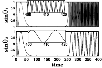
Figure 1: Top: Time series of $w_{1}$ (dotted line), $w_{18}$ (dashed line) and $w_{{\rm others}}$ (slid line). Middle & Bottom: Time series of $\sin(\theta_{1})$ and $\sin(\theta_{2})$. $N=20,\alpha=0.1$. Oscillator 1 and 18 separate to form a smaller cluster, thus a 2:18 clustering state emerges. The convergence ratio of $w_{i}$ between the clusters agrees with the inverse of the ratio of oscillators numbers (4).

Figure 2: The size of the largest cluster is plotted as a function of the variance of the initial conditions. The variance of $\theta$ is fixed to $10^{-2}$ and the variance of $w$ is bounded by $10^{-4}\leq\sigma_{w}\leq 10^{-1.5}$ . 1000 samples are tested for each value. The numbers in the figure represent the cluster-sizes obtained and, as can be seen, initial conditions closer to the one-cluster state yield larger uniform clusters, broadening the spread of the time scales.

The properties of the model can be summarized as follows; (i) a single coherent state is unstable and splits into some groups, (ii) clusters in split states are stable, (iii) the fraction of frequencies fulfills the condition (4) which generates the hierarchy of time scales from multi-clusters structures.

Since the interacting term only affects the variance of $w_{i}$, items (i) and (ii) concerning the coherence in $\theta_{i}$ reveal nontrivial properties. These are discussed in detail below. First, however, let us consider item (iii) which has a clear mechanism.

The frequencies of the clusters in a steady state are regulated by the states themselves. Since the couplings among synchronized oscillators have no effect, the $w_{i}$ of an oscillator that joins a cluster is activated by oscillators that don’t join the cluster. As $\alpha$ is set to $0.1$ and the variation of $w_{i}$ is slower than that of $\theta_{i}$, the effect of the coupling $1-\cos(\theta_{i}-\theta_{j})$ is averaged over time, and the averaged frequencies are proportional to the number of oscillators that do not join the clusters. Therefore, when two clusters with $n$ and $m$ oscillators coexist, the ratio of the averaged frequencies ($\overline{w}_{n}/\overline{w}_{m}$) fulfills the condition (4). Applying this discussion to multi-clusters states, where there are $l$ clusters with $n_{1},\cdots,n_{l}$ oscillators respectively ($\sum n_{i}=N$), the relation between averaged frequencies is

$$\frac{\overline{w}_{n_{i}}}{\overline{w}_{n_{j}}}=\frac{N-n_{i}}{N-n_{j}}.$$ (5)

Thus, multi-clusters states leads to multi-frequencies.

In order to analyze how the one cluster state becomes unstable and how the multi-clusters states emerge, corresponding to (i) and (ii), we now introduce a reduced description of the system.

To investigate the stability of the one cluster state, we take a two-cluster state as the initial condition,

$$\left\{\begin{array}[]{l}w_{i}=w_{f},~{}~{}\theta_{i}=\theta_{f}~{}~{}~{}~{}i=1,\dots,m\\ w_{j}=w_{s},~{}~{}\theta_{j}=\theta_{s}~{}~{}~{}~{}j=m+1,\dots,N\end{array}\right\}$$ (8)

$$(N=m+n,~{}~{}~{}n>m)~{}~{}~{}~{}~{}~{}~{}~{}$$

so that the system reduces to four variables. If we then introduce the relative coordinate

$$\omega=w_{i}-w_{j},~{}~{}~{}~{}\xi=\theta_{i}-\theta_{j},$$ (9)

the description can be further reduced to only two variables in cylindrical phase space,

$$\left\{\begin{array}[]{ll}\dot{\xi}=\omega\\ \dot{\omega}=A\{1-\cos(\xi)\}-\alpha\omega\end{array}\right.$$ (12)

$$A\equiv\frac{n-m}{N}.~{}~{}~{}~{}~{}~{}~{}~{}~{}~{}~{}~{}~{}~{}~{}~{}~{}~{}$$ (13)

The phase space of the $(\xi,\omega)$ system and the null cline are shown in Fig. 3, where the origin corresponds to the one cluster state .

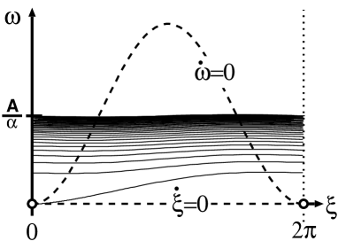
Figure 3: Phase space of the two clusters description in relative coordinates. Open circles denote the one cluster state, and the dotted line ($\xi=2\pi$) coincides with the line $\xi=0$ to form the cylindrical phase space. Null clines (dashed lines) and typical orbits separating from the one cluster state (thin solid lines) are also plotted . The orbit converges around $\omega=A/\alpha$.

Expanding equation (12) at the origin, we obtain

$$\left\{\begin{array}[]{l}\dot{\xi}=\omega\\ \dot{\omega}=-\alpha\omega+A\xi^{2}+O(\xi^{4})\end{array}\right..$$ (16)

The vector field at the origin has a zero and a negative eigenvalue, but when considering the second order we find that the origin, the one cluster state, is unstable.

The stable solution of the two clusters state $\overline{\omega}=\omega_{\alpha}(\xi)$, which is a limit cycle circling around the cylinder, is calculated as follows: When averaging $\cos(\xi)$ in (12), a limit cycle exists around the averaged line $\overline{\omega}=\frac{A}{\alpha}$, and $d\omega/d\xi\sim\alpha\ll\overline{\omega}$ indicates that the variation from the average is small (see Fig. 3). Then, by substituting the solution expanded in $\alpha$ into $d\omega/d\xi=\dot{\omega}/\dot{\xi}$ and by comparing the both sides, we obtain

$$\omega=\frac{A}{\alpha}-\alpha\sin(\xi)+O(\alpha^{3}).$$ (17)

which is in fairly good accordance with the numerical simulation.

In order to discuss the stability of the clusters in the two clusters state, we divide a cluster of them virtually and again describe the displacements with relative coordinates. Suppose a cluster containing $n$ oscillators is divided into two clusters with $n_{1},~{}n_{2}$ oscillators ($n=n_{1}+n_{2}$). Let $\epsilon$ and $\delta$ be the differences of the phases and the frequencies between the clusters respectively. Because our concern is the linear stability of the cluster, we focus on the region with sufficiently small $\epsilon$ and $\delta$. The previously employed coordinates $(\xi,\omega)$ are then naturally defined as the differences between the center of the divided clusters and the other cluster,

$$\left\{\begin{array}[]{l}\dot{\xi}=\omega\\ \dot{\omega}=A\left\{1-\cos(\xi)\cos(\frac{\delta}{2})\right\}\\ ~{}~{}~{}~{}~{}+B\sin(\xi)\sin(\frac{\delta}{2})-\frac{n}{2N}\{1-\cos(\delta)\}-\alpha\omega\\ \end{array}\right.$$ (21)

$$\left\{\begin{array}[]{l}\dot{\delta}=\epsilon\\ \dot{\epsilon}=-\frac{2m}{N}\sin(\xi)\sin(\frac{\delta}{2})+B\{1-\cos(\delta)\}-\alpha\epsilon\end{array}\right.$$ (24)

$$B\equiv\frac{n_{2}-n_{1}}{N}$$ (25)

The origin of the $(\delta,\epsilon)$ plane corresponds to the two clusters state. The region $|\delta|,|\epsilon|\ll 1$ is considered, and the behaviors of $\xi$ and $\omega$ are approximated by the solution of (17). Linearizing (24) at the origin, we obtain

$$\left\{\begin{array}[]{l}\dot{\delta}=\epsilon\\ \dot{\epsilon}=-\frac{m}{N}\sin(\xi)\delta-\alpha\epsilon\end{array}\right..$$ (28)

Here, $\sin(\xi)$ can be treated as a forced oscillation term that is approximated as

$$\xi \simeq \frac{A}{\alpha}t+\frac{\alpha^{2}}{A}\cos\left(\frac{A}{\alpha}t\right)$$

$$\sin(\xi) \simeq \frac{\alpha^{2}}{2A}+\sin\left(\frac{A}{\alpha}t\right)+\frac{\alpha^{2}}{2A}\cos\left(\frac{2A}{\alpha}t\right),$$ (29)

where $\dot{\xi}=\omega\simeq\frac{A}{\alpha}-\alpha\sin(\xi)$ is integrated by using successive approximations.

If a normal averaging method is applied, only the first constant term in (29) is taken to estimate the stability of (28). However, the amplitude of the oscillation in second term is much larger than that of the first term (in the order of the square of $\alpha$), and hence both terms should be included. Thus equations (28) can be expressed as

$$\ddot{\delta}+\alpha\dot{\delta}+\frac{m}{N}\left(\frac{\alpha^{2}}{2A}+\sin(\frac{A}{\alpha}t)\right)\delta=0.$$ (30)

Setting $\delta=R(t)\exp\{-\frac{\alpha}{2}t\}$, we obtain the Mathieu equation,

$$\ddot{R}+(p-2q\sin(2t))R=0$$ (31)

$$\left\{\begin{array}[]{l}p=\frac{\alpha^{4}}{A^{2}}\left(\frac{2m}{AN}-1\right)\\ q=\frac{2\alpha^{2}m}{A^{2}N}\end{array}\right.$$ (34)

Here, $p=O(\alpha^{4})\ll 1,~{}q=O(\alpha^{2})\ll 1$ is in the area of Mathieu’s parameters where $R=0$ is stable. Since $\delta$ is the product of $R$ and the exponential decay term $\exp\{-\frac{\alpha}{2}t\}$, $\delta$ is not destabilized by the $O(\alpha^{2})$ perturbation which is omitted to approximate $\sin(\xi)$. Therefore the clusters in the two clusters state can be concluded to be stable.

In the present paper we introduce a novel type of coupled oscillator model where the time scales occur as variables. It is shown that multiple clusters with different time scales emerge through a self-organization process based on time scale plasticity. This process is characterized by symmetry breaking due to separation from the one-cluster state.

Though we introduce our model (3) as one of the simplest model to discuss time scale plasticity, which is also derived from a limit-cycle model with some assumptions, Suppose we have globally coupled limit cycles of normal form type in polar coordinates

$$\left\{\begin{array}[]{l}\dot{\theta_{i}}=b(1-r_{i}^{2})+\frac{1}{N}\sum\frac{r_{j}}{r_{i}}\sin(\theta_{j}-\theta_{i})\\ \dot{r_{i}}=ar_{i}(1-r_{i}^{2})+\frac{1}{N}\sum\left(\cos(\theta_{j}-\theta_{i})r_{j}-r_{i}\right),\end{array}\right.$$ (37)

where the coordinate is chosen that the angular velocity becomes zero at the limit cycle. Then we assume $b\gg a\gg D$, transform $r_{i}=1-O(D/a)\equiv 1-w_{i}$ and omit the terms of $O(D/b)$ and $O(D^{2}/a^{2})$,

$$\left\{\begin{array}[]{l}\dot{\theta_{i}}=-2bw_{i}\\ \dot{w_{i}}=-2aw_{i}+\frac{D}{N}\sum\left(1-\cos(\theta_{j}-\theta_{i})\right)\end{array}\right.$$ (40)

is obtained. Lastly with appropriate transformations, equation (3) is derived. In this setup, the time scale of the each oscillator diverges at the limit cycle, and the plasticity results from the steep gradient of frequencies ($b\gg D$) around the cycle. In this way, such singular properties can also lead the plastic time scales Tac03 .

Figure 4: Time series data of $\omega_{i}$ from a highly spread initial condition. Neither a large cluster nor large differences between $w_{i}$ emerge and the whole system continues to be chaotic.

Another type of multiple frequency behavior in coupled oscillators is studied in the context of antenna and radar systems in In03 where the hierarchy is characterized by a discrete symmetry group of the system. Although those hierarchies and the ones reported here have different mechanisms, a unified explanation should be developed for these structures. Since we use the simplest oscillator as the dynamical element, a hierarchy with only a few layers is observed. In more complex systems of chaotic oscillators, multiple layers can be self-organized (to be reported in a forthcoming paper FT04 ). In this study, the initial conditions are restricted to the vicinity of the one-cluster state. When we choose more scattered out initial conditions, coherent structures do not emerge, chaotic behaviors persist and large time scale differences are not generated (Fig. 4). This implies the importance initial condition selection, a requirement common to many self-organization phenomena in highly complex systems FK00 .

The authors are grateful to A. Awazu, H. Daido, T. Ikegami, K. Kaneko, S. Sasa, F. H. Willeboordse and H. Yamada for useful discussions. This work is supported by a Grant-in-Aid for Scientific Research from the Ministry of Education, Science, and Culture of Japan.

References

- (1) G. Buzsaki and A. Draguhn, Science, 304, 1926 (2004).
- (2) J. Keener and J Sneyd, Mathematical Physiology, (Springer-Verlag, 1998); D. Fell, Understanding the Control of Metabolism, (Portrand Press, 1997).
- (3) E. Korobkova et al., Nature, 428, 574, (2004).
- (4) Y. Nakaoka et al., Proc. Jpn. Acad., 58, 213 (1982).
- (5) K. Fujimoto and K. Kaneko, Physica D 180, 1 (2003); K. Fujimoto and K. Kaneko, Chaos 13, 1041 (2004).
- (6) A. V. Egorov et al., Nature, 420, 173 (2002).
- (7) T Shinjo et al., Physica D, 84, 212 (1995); Y. Adachi et al., J. Immunol, 163, 4367 (1999); A. J. Rosenspire et al., Biophys. J., 79, 3001, (2000); L. B. Dale et al., J. Biol. Chem. 276, 35900, (2001); L. F. Olsen et al., Biophys. J., 84, 69, (2003).
- (8) A. Takamatsu et al., J. Phys. Soc. Jpn. 66 1638 (1997).
- (9) G. Nicolis and I. Prigogine, Self- organization in nonequilibrium systems, (New York: John Wiley & Sons, 1977).
- (10) A. T. Winfree, The Geometry of Biological Time, (Springer, New York, 1980); Y. Kuramoto, Chemical Oscillations, Waves, and Turbulence, (Springer, Berlin, 1984); K. Kaneko and I. Tsuda, Complex Systems : Chaos and Beyond (Springer, Tokyo, 2001).
- (11) M. Tachikawa, Prog. Theor. Phys., 109, 133 (2003).
- (12) V. In et al., PRL, 91, 244101 (2003).
- (13) K. Fujimoto and M. Tachikawa, in preparation.
- (14) C. Furusawa and K. Kaneko, J. Theor. Biol., 209, 395, (2001).