Spectral fluctuations and 1/f noise in the order-chaos transition regime

Abstract

Level fluctuations in quantum system have been used to characterize quantum chaos using random matrix models. Recently time series methods were used to relate level fluctuations to the classical dynamics in the regular and chaotic limit. In this we show that the spectrum of the system undergoing order to chaos transition displays a characteristic $f^{-\gamma}$ noise and $\gamma$ is correlated with the classical chaos in the system. We demonstrate this using a smooth potential and a time-dependent system modeled by Gaussian and circular ensembles respectively of random matrix theory. We show the effect of short periodic orbits on these fluctuation measures.

Quantum chaos, the study of quantum analogues of classically chaotic systems, is characterized by the fluctuation properties of the spectrum of its Hamiltonian operator. For quantum systems with regular classical dynamics the spectral fluctuations are Poisson distributed bt , i.e, the eigenvalues tend to cluster together. On the other hand, one of the remarkable results established by Bohigas et al is that the level fluctuation properties of quantum systems, whose classical limit is chaotic, are identical to those of an appropriate ensemble from random matrix theory (RMT) boh1 . This is the level repulsion regime where the eigenvalues tend to repel one another. In this sense, characterizing quantum chaos in terms of presence or absence of level repulsion requires invoking the spectral properties of random matrix ensembles. Recently, in analogy with time series, a method has been proposed to characterize spectral fluctuations using inherent properties of the spectrum rel1 . If the eigenvalues of Hamiltonian operators could be thought of as a time series and its index the time in some units, then the methods of traditional time series analysis can be applied to it. It was shown that the ensemble averaged power spectrum $\langle S(f)\rangle$ of the fluctuations in the cumulative level density, goes as $1/f$ or $1/f^{2}$ depending on whether the system is classically chaotic or regular rel2 . This work also showed examples of atomic level sequences displaying $1/f$ noise. Thus, atomic levels join the host of other systems and phenomena that display $1/f$ noise lending strength to the well known cliché that $1/f$ noise is ubiquitous in nature obf .

In this paper, we study the transition from regularity to chaos in the mixed systems. In such systems the regular and chaotic motion coexist and this is a generic feature. For instance, the entire class of atoms in strong fields and the range of problems involving atoms in time-varying fields belong to this class. We study a smooth Hamiltonian system, the quartic oscillator and a time dependent system, the kicked top. In both these systems, a single parameter that controls the classical chaos can be varied to get a smooth transition from regular to predominantly chaotic dynamics. It is well known that the level fluctuations in these systems can be modelled by RMT boh1 . From an RMT point of view, these models possess symmetries (time-reversal invariance without spin-1/2 interactions) such that the kicked top is part of the circular orthogonal ensemble whereas the coupled oscillator falls in the Gaussian orthogonal ensemble (GOE) of RMT rmt . Based on the numerical evidence from these models we show that $\langle S(f)\rangle\;\varpropto f^{-\gamma}$, where $\gamma$ depends on the degree of their classical chaos. This correlation between $\gamma$ and the classical chaos parameter is established using semi-empirical level spacing distributions studied in the context of RMT to model the transition region.

In semiclassical systems of the type we consider here, periodic orbits via the Gutzwiller formalism play an important role in determining the quantum spectrum rmt . As pointed out by Berry ber1 , the properties of the spectrum on a scale of mean level spacing are determined by long time period orbits and in a sense both of them display universality; the RMT type universality in the spectrum and classical universality embodied in the Hannay-Ozorio sum rule hor . However, long range spectral properties are determined by the short time periodic orbits which are system specific and are not universal. This manifests itself in the power spectrum as deviations from the $f^{-\gamma}$ behavior. We show the effect of short time periodic orbits in the coupled oscillator, where scarring or the density enhancements in the vicinity of certain periodic orbits hell is a prominent feature due to these orbits.

The Hamiltonian for the coupled quartic oscillator is,

$$H_{1}=p^{2}_{1}+p^{2}_{2}+q_{1}^{4}+q_{2}^{4}+\alpha~{}q_{1}^{2}q_{2}^{2}.$$ (1)

This system is classically integrable for $\alpha=0,2,6$ and the phase space is predominantly chaotic for $\alpha>6$. This has been extensively studied as a model for chaotic dynamics in a smooth potential qo ; eck . The Hamiltonian is quantized by solving the corresponding Schrödinger equation in the basis of the eigenfunctions corresponding to $\alpha=0$. Then, the matrix elements of Hamiltonian operator $\widehat{H}_{1}$ is computed in this basis and the matrix of order 13000 is diagonalized to obtain about 2000 converged eigenvalues. This system possesses $C_{4v}$ point group symmetry. We symmetry decompose the spectrum and study the levels from only the $A_{1}$ irreducible representation.

The quantum top top1 is characterized by an angular momentum vector ${\bf J}$, whose components $(J_{x},J_{y},J_{z})$ obey the usual commutation relations and ${\bf J^{2}}=j(j+1),j=\frac{1}{2},1,\frac{3}{2}$,……, is conserved. The dynamics of the top is governed by the Hamiltonian top1 , $H_{2}(t)=\frac{\pi}{2}J_{y}+\frac{k}{2j}J_{z}^{2}\sum_{n}\delta(t-n)$. The first term describes the precession around the $y$ axis with angular frequency $\pi/2$ and the second term kicks in periodically with $\delta$-function kicks of strength $k$. Each kick can be thought of as an impulsive rotation about $z$-axis by an angle $kJ_{z}/2j$. The time evolution operator in between consecutive kicks is,

$$U=\exp\left(-i\frac{k}{2j}J_{z}^{2}\right)\exp\left(-i\frac{\pi}{2}J_{y}\right).$$ (2)

If $e^{i\phi}$ are the eigenvalues of $U$, then the power spectrum is computed from the quasienergy $\phi$. In the limit $j\rightarrow\infty$, we can derive a classical map whose dynamics depends on the parameter $k$ top1 . At $k=0$ it is integrable and becomes increasingly chaotic for $k>0$.

We denote the eigenvalues of the appropriate operator described above by $E_{i}$, $i=1,2,\dots,n+1$. The integrated level density, that counts the number of levels below a given $E$, can be decomposed into an average and an oscillating part, $N(E)=\overline{N}(E)+N_{osc}(E)$. In order to compare the fluctuations from various systems it is customary to unfold the spectrum by a transformation $\lambda_{i}=\overline{N}(E_{i})$, such that the mean level density of the transformed levels is unity. All further analysis is carried out using the sequence $\{\lambda\}$. For instance, the spacing is $s_{i}=\lambda_{i+1}-\lambda_{i},i=1,2,\dots,n$. In this paper, we will work with the statistic given by,

$$\delta_{m}=\sum_{i=1}^{m}(s_{i}-\langle s\rangle)\equiv-N_{osc}(E_{m+1})\;\;\;\;\;\;m=1,2,...n$$ (3)

Once the unfolding is performed, on an average, a unit interval of the spectrum will have one level. Hence, $\delta_{m}$ represents the cumulative deviation until $m$th level, of the $i$th unfolded level from $i$. This quantity has a formal analogy with a time series. If the index $i$ represents the (scaled) time, then $(s_{i}-\langle s\rangle)$ represents the actual value assumed by the series at the $i$th time instant. Following Ref. rel1 , we take the power spectrum of $\delta_{m}$ as,

$$S(f)=|\widehat{\delta}_{f}|^{2}=\left|\frac{1}{\sqrt{n+1}}\sum_{m}\delta_{m}\exp\left(\frac{-2\pi ifm}{n+1}\right)\right|^{2}$$ (4)

where $f=1,2,\dots,n;\,\,\widehat{\delta}_{f}$ is the Fourier transform of $\delta_{m}$. Now, we will present results to infer that $\langle S(f)\rangle\varpropto f^{-\gamma}$ and $\gamma$ depends on the degree of chaos in the system.

Before we plunge into the results, we show the statistic $\delta_{m}$ for our models. For the quartic oscillator, using the results in Refs. mart we symmetry decompose the level density to obtain the asymptotic integrated level density for the $A_{1}$ representation,

$$\begin{split}\overline{N}_{A_{1}}(E)&\approx\frac{1}{8}\left[\frac{E^{3/2}}{6}F\left(\frac{1}{2},\frac{1}{2};1;\frac{2-\alpha}{4}\right)\right.\\ +&\left.\frac{\Gamma(5/4)E^{3/4}}{\Gamma(7/4)\sqrt{\pi}2^{7/4}}+\frac{E^{3/4}}{\Gamma(7/4)\sqrt{2\pi}(2+\alpha)}+\frac{3}{4}\right]\end{split}$$ (5)

where $F(.)$ is the Gauss’ Hypergeometric function. We use this expression to unfold the quartic oscillator levels.

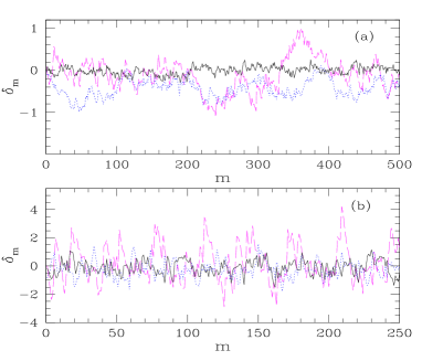
Figure 1: (Color online) $\delta_{m}-m$ curve for (a) kicked top and (b) quartic oscillator. The solid curve corresponds to chaotic case $(k=7,\alpha=20)$ and the dotted curve to the intermediate region $(k=3,\alpha=12)$, and the dashed curve to regular limit $(k=1,\alpha=0)$.

Fig. 1 displays $\delta_{m}-m$ for the quartic oscillator and the kicked top for a choice of 3 parameters in the regular, chaotic and the transition region. In Fig. 1(a) for the kicked top, the dashed curve corresponding to nearly the Poisson spectrum ($k=1$) differs markedly from the solid curve for almost the GOE $(k=7)$ limit. We also plot an intermediate case (dotted curve) to show the transition taking place from Poisson to GOE type spectrum. This intermediate case at $k=3$ is also qualitatively different. Each series displays slightly different memory effects corresponding to various shades of anti-persistent time series. In fact, such time series are known to display $f^{-\gamma}$ noise and we expect similar result based on this analogy. We observe similar features for the quartic oscillator in Fig. 1(b) for $\alpha=6,11.5,19.5$, as reported in an earlier work of Bohigas boh2 .

In Figs. 2 and 3, we display the ensemble averaged power spectrum of $\delta_{m}$. Ensemble averaging is done as follows : for each $\alpha$ of the quartic oscillator we obtain 2000 levels. After leaving out the first 200 levels, we create 3 sequences of 600 levels each. We further obtain similar sequences from more values of $\alpha$ separated by $\delta\alpha=0.1$. For instance, $\alpha=11.5$ in Fig. 3(b) corresponds to ensemble average in the range $\alpha=11.2-11.8$ in steps of 0.1. Hence, the results (except for the integrable case in Fig. 3(a)) represent an average over 21 level sequences of length 600 each. For the integrable case, the ensemble consists 9 level sequences (3 from each of $\alpha=0,2$ and 6) of length 600 each. Similar averaging is done for the kicked top with 11 level sequences of length 800 each.

Figure 2: Power spectrum of $\delta_{n}$ for kicked top at (a) $k=1$, (b)$k=2.0$, (c) $k=3.0$ and (d) $k=7.0$. The solid line is the least squares fit. The slope $\gamma$ is indicated in each graph.

For the regular and chaotic limits shown in Figs. 2(a,d) and 3(a,d), there is a good agreement with the predicted slopes of $\gamma=2,1$ respectively rel2 . There are deviations for $f<f_{\mbox{\small min}}$ due to the effect of short periodic orbits with scaled time period $f_{\mbox{\small min}}$. The deviation for large $f$ arises, partly, from approaching the Nyquist frequency at $f=(n+1)/2$. It is clear from Figs. 2,3(b,c) that as the oscillator and the top explore the intermediate region between the regular and the chaotic limits, the slope $\gamma$ smoothly changes from 2 to 1. Intuitively, we can expect this because other statistic’ in the transition regime, e.g, spacing distribution, generally vary smoothly too in this regime.

Figure 3: Power spectrum of $\delta_{m}$ for quartic oscillator at (a) $\alpha$=0, 2,6 (b) $\alpha$=7.5 (c) $\alpha$=11.5 and (d) $\alpha$=19.5 . The solid lines are the least squares fit with intercept shifted for clarity. The slope $\gamma$ is indicated in each graph. The arrows in (b-d) indicate $\log f_{\mbox{\small min}}$, the time period of the short periodic orbit.

In order to obtain a global picture, we compute the exponent $\gamma$ for a range of parameter values of $\alpha$ and $k$ in the order-chaos transition region. In RMT, this transition is described by a semi-empirical spacing distribution $P(s;\beta)$ characterised by the parameter $\beta$. As $\beta$ is varied from 0 to 1, $P(s;\beta)$ changes smoothly from Poisson to GOE, reflecting the change in classical dynamics from regularity to chaos. Here, we use the distribution $P_{T}(s;\beta)$ due to Izrailev izr . For $\beta=0$, $P_{T}(s;\beta)$ gives a Poissonian form (integrable limit) and for $\beta=1$ it closely approximates the GOE distribution (chaotic limit). The intermediate values, $0<\beta<1$, correspond to order-chaos transition. Fig. 4(a,b) shows that the series of $\beta$ and $\gamma$ display similar trends and are strongly correlated for both the top and the oscillator. It is known that the fraction of regular regions in phase space is correlated with a parameter like $\beta$ that characterizes the change in spacing distribution zimm . Hence we infer that the exponent $\gamma$ in the power spectrum reflects the qualitative trends in the classical dynamics of the system. In general, we have shown that $\langle S(f)\rangle\varpropto f^{-\gamma}$, where the value of $1\leq\gamma\leq 2$ relates to the nature of classical dynamics for the oscillator and the top.

As opposed to purely random matrices, the semiclassical systems deviate from $f^{-\gamma}$ scaling rel2 for $f<f_{\mbox{\small min}}$, where $f_{\mbox{\small min}}$ is the period $t_{\mbox{\small min}}$ of the shortest periodic orbit (PO) scaled by the Heisenberg time $(t_{H}=2\pi\hbar)$ ber1 , i.e, $f_{\mbox{\small min}}=(n+1)t_{\mbox{\small min}}/t_{H}$. This corresponds to short POs being system specific features and in the corresponding large energy scales universality breaks down leading to deviations from RMT based results ber1 . Since the spectral form factor is linear only for times $t/t_{H}<1$, which is necessary to realise $1/f$ noise rel2 , the actual range of scaling is restricted to $f_{\mbox{\small min}}\ll f\ll f_{H}$. Since all times are scaled by $t_{H}$, at $t=t_{H}$, we have $f_{H}=(n+1)$. The short PO in the quartic oscillator is the ‘channel orbit’, as it is referred to in the literature, with the initial condition $(q_{1}=0,q_{2},p_{1}=0,p_{2})$. This can be identified by taking discrete Fourier transform of the scaled energies of the oscillator boh2 . The period of this orbit is $t(E)=E^{-1/4}\frac{\sqrt{\pi}\Gamma(1/4)}{2\;\Gamma(3/4)}$. Among all the sequence of levels that form the ensemble let the largest level be $E=E^{\prime}$. Then, the period of the short PO is $t_{min}=t(E^{\prime})$. For instance, at $\alpha=11.5$, we have $E^{\prime}=2579.05$ ($\hbar=1$) and $n=600$ and this provides the theoretical bounds for scaling to be $\log(f_{min})=1.54$ and $\log(f_{H})=2.77$, as indicated in Fig. 3(c). It is evident from Fig. 3(b-d) that $\langle S(f)\rangle\varpropto f^{-\gamma}$ in almost the entire theoretically expected range $f_{\mbox{\small min}}\ll f\ll f_{H}$. This scaling range can be increased by probing deep in the semiclassical ($\hbar\to 0$) regime, since $t_{H}\backsim\hbar^{-1}\backsim E^{3/4}$ for the quartic oscillator. But this leads to large eigenvalue problems that may not be computationally feasible at present.

Figure 4: The parameter $\beta$ (squares) in $P_{T}(s)$ as a function of chaos parameter for (a) the kicked top and (b) quartic oscillator. Also plotted is the shifted slope $2-\gamma$ (circles) of the power spectrum $\langle S(f)\rangle$. The slope is shifted such that $y-$axis lies in the range 0 to 1.

In Fig. 5, we show the effect of short periodic orbits on the power spectrum of $\delta_{m}$. Note that for the quartic oscillator at $\alpha=20$, $\gamma=1.073$ whereas for $\alpha=30$ we have $\gamma=1.322$ and $\beta$ also shows a similar trend (see Fig 4). In general, we would expect that as $\alpha$ increases monotonically, chaos also increases and hence agreement with RMT should get better. But numbers quoted above show that, roughly speaking, chaos at $\alpha=20$ is more than at $\alpha=30$. This ‘anomalous’ feature is the effect of oscillating stability of the short PO. At $\alpha=20,30$ the short PO undergoes an anti-pitchfork and a pitchfork bifurcation respectively accompanied by local changes in the phase space structure mss2 . This, in turn, affects the spectral levels. It is known that the short POs influence a series of eigenstates, called the localized or sometimes the scarred states, in the quartic oscillator spectrum and they deviate strongly from RMT for eigenvector statistics eck ; san ; mss . If we remove the spacings that involve localized states, then we might expect the resulting distribution to show a better agreement with RMT. This is like removing the effect of short POs in the spectrum. The dotted line in Fig. 5 is the usual power spectrum and the solid line is the one whose spacings involving localised states are removed. In this example the ensemble has just 3 sequences of 600 levels each which is reflected in large amplitude of fluctuations. The power spectrum changes character for $f<f_{\min}$ and the range of validity of power law gets better. This is a manifestation of the effect of short POs in the spectrum.

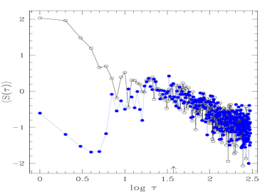
Figure 5: (Color online) The effect of short periodic orbits in the spectrum. $\langle S(f)\rangle$ for quartic oscillator at $\alpha=30$ including the localized states (dotted). The arrow indicates $f_{\mbox{\small min}}$. The solid line is the power spectrum after localized states are removed.

In summary, we have shown that the spectral fluctuations in the quartic oscillator and the kicked top display $f^{-\gamma}$ noise, where the value of $\gamma$ within the limits $1\leq\gamma\leq 2$ reflects the underlying nature of classical dynamics, namely, regular or chaotic or a mixture thereof. We show the effect of short POs on the spectral fluctuations. We expect $f^{-\gamma}$ type noise in the level fluctuations to be an inherent characteristic of quantum systems.

- (1) M. V. Berry and M. Tabor, Pro. R. Soc. Lond. A 356, 375 (1977).
- (2) O. Bohigas et. al., Phys. Rev. Lett. 52, 1 (1984).
- (3) A. Relao et. al., Phys. Rev. Lett. 89, 244102 (2002); S. N. Evangelou et. al., Phys. Lett. A 334 331 (2005).
- (4) E. Faleiro et. al., Phys. Rev. Lett. 93, 244101 (2004).
- (5) Bruce J. West and M. F. Shlesinger, American Scientist 78, 40 (1990).
- (6) F. Haake, Quantum Signatures of Chaos, 2nd ed. (Springer-Verlag, Berlin, 2000).
- (7) M. V. Berry, Proc. R. Soc. Lond. A 422, 7 (1989).
- (8) J. H. Hannay and A. M. O. de Almeida, J. Phys. A 17, 3429 (1984).
- (9) E. Heller, Phys. Rev. Lett. 53, 1515 (1984).
- (10) O. Bohigas et al, Phys. Rep. 223, 43 (1993).
- (11) B. Eckhardt et al, Phys. Rev. A 39, 3776 (1989).
- (12) F. Haake et al, Z. Phys. B 65, 381 (1987).
- (13) S. G. Matinyan and Y. Jack Ng, J. Phys. A 36, L417 (2003); N. D. Whelan J. Phys. A 30, 533 (1997).
- (14) O. Bohigas in Chaos and Quantum Physics, eds. M.-J. Giannoni et al, (North-Holland, 1991).
- (15) F. M. Izrailev, Phys. Lett. A 134, 13 (1988); J. Phys. A 22, 865 (1989); G. Casati et al, J. Phys. A 24, 4755 (1991).
- (16) Th. Zimmermann et. al., Phys. Rev. A. 33, 4334 (1986).
- (17) H. Yoshida, Cell. Mech. 31 363 (1983) ; M. Brack et al, J. Phys. A 36, 1095 (2003); M. S. Santhanam et al, Phys. Rev. Lett. 76 396 (1996).
- (18) M. S. Santhanam et al, Phys. Rev. E 57, 345 (1998).
- (19) M. S. Santhanam et al, Pramana 48, 439 (1997).
- (20) J. M. G. Gomez et al, cond-mat/0502130.