Discrete peakons

Abstract

We demonstrate the possibility for explicit construction in a discrete Hamiltonian model of an exact solution of the form $\exp(-|n|)$, i.e., a discrete peakon. These discrete analogs of the well-known, continuum peakons of the Camassa-Holm equation [Phys. Rev. Lett. 71, 1661 (1993)] are found in a model different from their continuum siblings and from earlier studies in the discrete setting [Phys. Rev. Lett. 83, 248 (1999)]. Namely, we observe discrete peakons in Klein-Gordon-type and nonlinear Schrödinger-type chains with long-range interactions. The interesting linear stability differences between these two chains are examined numerically and illustrated analytically. Additionally, inter-site centered peakons are also obtained in explicit form and their stability is studied. We also prove the global well-posedness for the discrete Klein-Gordon equation, show the instability of the peakon solution, and the possibility of a formation of a breathing peakon.

I Introduction

In the last two decades, intrinsic localized modes (ILMs), also termed discrete breathers (DBs), have become a topic of intense theoretical and experimental investigation; see, e.g., review for a number of recent reviews on the topic. Per their inherent ability to bottleneck and potentially transport the energy in a coherent fashion, such exponentially localized in space and periodic in time entities have come to be of interest in a variety of contexts. These range from nonlinear optics and arrays of waveguides mora to Bose-Einstein condensates (BECs) inside optical lattice potentials tromb and from prototypical models of nonlinear springs pesa to Josephson junctions alex and dynamical models of the DNA double strand Peybi .

The ubiquitous nature of nonlinear lattice systems (i.e., arrays of coupled nonlinear oscillators) has prompted the examination of the behavior of nonlinear waves in these systems, particularly for the waves that are well-known and understood in the continuum analogs of these equations i.e., in nonlinear partial differential equations. In this direction of activity, many of the coherent, nonlinear wave structures that have previously been discovered in continuum settings such as regular solitons malomed , compactons rosenau , shock waves shocks or gap solitons chen have been recently examined in the discrete setting; see, e.g., the works of review for regular solitary waves, johan for discrete compactons, konotop for discrete shock waves or andrey for lattice gap solitons.

On the other hand, a continuum nonlinear wave that was recently obtained in the context of shallow water wave equations, namely the peakon (a peaked soliton solution with a discontinuity in the first derivative at its peak) only very recently started to be considered in the discrete contextoster . Peakons were given their name (in the context of the so-called Camassa-Holm equation, which is a dispersive, integrable model ch1 ; ch2 ) due to their discontinuous derivative at peak amplitude. It is worth noting, however, that such “sharply pointed” structures were also obtained much earlier in the context of nonlocal models for plasmas (see, e.g., litvak ). While, at first glance, it may not appear particularly natural to have discrete analogs of these solutions, as derivatives are not, strictly speaking, defined in the context of the spatial lattice, our aim in the present work is to examine the “discrete peakon”. This will be a lattice profile in the form (in fact, exactly) $\sim\exp(-a|n|)$ that in the continuum limit will asymptotically approach the continuum peakon solution.

A number of twists accompany this discrete peakon solution introduced here. In the discussion, we will illustrate that glimpses of solutions that can be categorized under this new “species” may have already appeared in a somewhat generalized form in earlier works. We hope this may initiate a more general examination of the presently suggested lattice peakons. We believe that we have encapsulated the key mechanisms whose interplay can give rise to the existence of peakons (in both the discrete and the continuum setting) in a model of the Klein-Gordon (KG) variety and its nonlinear-Schrödinger (NLS) type analog. It is interesting to note that both the dispersive and the nonlinear terms that we have combined in the present setting have appeared previously in diverse contexts (that will be mentioned below); however, they were never combined to allow for the existence of peakons. Another intriguing bit concerns the stability properties of the peakons which are also examined in what follows. We find that the peakons, while unstable in the KG variant of our model, become stable in its NLS version. This is because the negative energy direction present the former model is prohibited by the charge conservation in the latter model. In the KG case, discrete breathing peakons are possible instead. Interestingly, such solutions were also identified earlier in closed form in a class of models very different than the ones examined herein [more specifically in a class of homogeneous, nearest neighbor, Klein-Gordon Hamiltonians] in flach . Finally, it is remarkable that the presently examined class of models and its stability features can be treated by methods available for the continuous nonlinear field equations as illustrated below.

Our presentation will be structured as follows. In Section II, we will discuss the model and its motivation. In Section III, the numerical results will be presented for site-centered, as well as for inter-site centered peakons. In Section IV, we will examine the stability of such structures through analytical considerations based on constrained energy minimization, as well as on functional analytic arguments. In Section V, the existence of discrete breathing peakons is discussed. Finally, in Section VI, we will summarize our findings and present our conclusions, as well as some open questions for future studies.

II Model and Motivation

Examining the peakon from the “reverse engineering” (or the inverse problem) point of view, we would like to use the properties of a solution of the form $u(x)\sim\exp(-|x|)$, to construct a (continuum as well as a) discrete lattice with dynamics that supports such peaked solutions. Adopting this viewpoint, some of the key properties of $u(x)=\exp(-|x|)$ are that

$$u^{\prime}(x)=-u(x){\rm sgn}(x),$$ (1)

$$(1-\partial_{x}^{2})u(x)=2\delta(x)u(x).$$ (2)

This second property (cf. also ch1 ) justifies why a strongly localized impurity (of the form of a $\delta$-function) may be a relevant context in which such peaked solutions could arise. We will return to this point in Section VI.

Another, perhaps more interesting for our purposes, property is the result of convolution of such a peaked function with a Kac-Baker exponential interaction kernel $J(|x-y|)=\exp(-|x-y|)$ kac ; baker . The convolution yields:

$$J\star u\equiv\int_{-\infty}^{\infty}\exp\left(-|x-y|\right)\exp(-|y|)dy=\left(1+|x|\right)\exp\left(-|x|\right).$$ (3)

This suggests immediately from a mathematical perspective a Klein-Gordon (KG), as well as a nonlinear Schrödinger (NLS) model with long-range interactions that would support exact peakon solutions of the form $u(x)=A\exp(-a|x|)$. In particular the KG model would read:

$$u_{tt}=a\int_{-\infty}^{\infty}\exp(-a|x-y|)u(y)dy-\left(1-\frac{1}{2}\ln\left(\frac{u^{2}}{A^{2}}\right)\right)u.$$ (4)

The peakons in this case would represent static solutions of the KG equation. The corresponding NLS model would be of the form

$$iu_{t}=-a\int_{-\infty}^{\infty}\exp(-a|x-y|)u(y)dy-\frac{1}{2}\ln\left(\frac{|u|^{2}}{A^{2}}\right)u,$$ (5)

wherein the peakons correspond to standing wave solutions of the form $u(x)=A\exp(it)\exp(-a|x|)$.

Continuing along this lane of reverse construction (the motivation for each of the relevant terms will be given below), we now explain that an interesting feature of the above considerations is that they can also be carried through in the discrete setting. In particular, for $u_{n}=\exp(-a|n|)$, we sum up the geometric series establishing that:

$$\sum_{m\in{\mathbb{Z}}}\exp(-a|n-m|)u_{m}=\left(\frac{\exp(2a)+1}{\exp(2a)-1}+|n|\right)u_{n}.$$ (6)

Consequently, for the discrete Kac-Baker interaction kernel

$$J_{nm}=\exp(-|n-m|),$$ (7)

we can devise a discrete KG, as well as a discrete NLS model that have discrete analogs of peaked solutions. The discrete KG model is of the form:

$$\ddot{u}_{n}=\sum_{m\in{\mathbb{Z}}}J_{nm}u_{m}-\left[\frac{\exp(2a)+1}{\exp(2a)-1}-\frac{1}{2a}\ln\left(\frac{u_{n}^{2}}{A^{2}}\right)\right]u_{n},$$ (8)

with the exact discrete peakon solution $\pi_{n}=A\exp(-a|n|)$, while the corresponding discrete NLS chain can be formulated as:

$$i\dot{u}_{n}=-\sum_{m\in{\mathbb{Z}}}J_{nm}u_{m}+\left[\frac{2}{\exp(2a)-1}-\frac{1}{2a}\ln\left(\frac{|u_{n}|^{2}}{A^{2}}\right)\right]u_{n},$$ (9)

where a discrete peakon given by the standing wave $\exp(it)\pi_{n}$ is the exact solution of the model.

It is these latter equations [Eqs. (8) and (9)] and their dependence on the parameter $a$ that determines the interaction “range” that we plan on investigating in what follows. Notice that $a$ can be considered as a natural spacing parameter.

It is interesting to note as a side remark (to which we will return in later sections) that this model not only supports an exact “on-site” discrete peakon solution such as the one given above, but additionally supports exact “inter-site” peakon solutions of the form: $u_{n}=B\exp(-|n-1/2|)$ for the Klein Gordon (in the DNLS case it is $u_{n}=B\exp(it)\exp(-|n-1/2|)$). The value of the prefactor $B$ is given by the relation

$$\ln(B/A)=a\left[\frac{(\exp(a)-1)}{2(\exp(a)+1)}\right].$$ (10)

Such explicit solutions (especially inter-site ones) are rarely available in non-integrable discrete models. Inter-site solutions are typically less stable than their on-site siblings ijmpb . In the present setting, we will study in detail the behavior of such two-site peakons numerically as well as analytically.

In motivating the model, aside from its intrinsic mathematical interest due to the existence of the peaked solutions (both in the discrete case and in the continuum limit), we should remark that both the dispersive and the nonlinear terms included here have appeared in a variety of settings before. The Kac-Baker type kernel kac ; baker , aside from its relevance in models of statistical physics, has been used quite extensively in recent nonlinear studies of lattice models emulating biopolymer dynamics including DNA; see, e.g., gaid1 ; gaid2 ; gaid3 ; gaid4 ; gaid5 ; gaid6 . Hence, this type of interaction is rather ubiquitous and can be controllably tuned (depending on the value of $a$), to be practically nearest neighbor (for large $a$) or much longer range (for $a\rightarrow 0$). Let us note also that in the past and in the framework of continuum equations similar forms of this kernel had been examined in the work of witham (but in a rather different dynamical model, namely one of the KdV type) wherein it was found that traveling waves acquired a peaked waveform. In contexts more closely related to the ones of the present work, let us also mention that “cusp solitons” (i.e., peakons) were also found in continuum models of the NLS type with Kac-Baker interactions in ybg (however, they were unstable) and in the case of a nonlocal Klein-Gordon field theory in egor .

The logarithmic nonlinearity in nonlinear model equations was originally introduced in the context of quantum field theory rosen . It reappeared in bb , where it was proposed as an equation for generalized quantum mechanics. Later in ms6 , it was suggested as a description for extended objects in nuclear matter, while more recently it was examined in the context of a scalar field model in inflationary cosmology cosmol . These studies have also triggered a more mathematically oriented interest in this nonlinearity and the properties of the solutions of the corresponding nonlinear wave equations maslov . Perhaps, most closely to the purposes of interest to this study, this type of logarithmic field theory has appeared in saturable nonlinear optical media. The initial investigations of sny in the latter context, in the framework of the “mighty morphing” spatial solitons, were later placed in a more physically realistic framework in connection with photorefractive materials in christo . The work of christo suggests that for the nonlinear waveguide evolution, the logarithmic nonlinearity provides an accessible model that offers valuable insight, while maintaining the characteristic features of the underlying physical process. A note of caution should however be made in this connection in that the nonlinearity of Eqs. (8)-(9) should be viewed as a more reasonable physical model for larger amplitudes (where it can be considered as an approximation of a more physical nonlinear term such as ${\rm ln}(1+|u_{n}|^{2})$). For amplitudes tending to $0$, the divergence of ${\rm ln}(|u_{n}|^{2})$ appears to be somewhat unphysical and leads to the absence of a small amplitude excitation (so-called “phonon”) spectrum.

The combination of the features of the dispersive interaction (its controllable range and wide applicability) and of the logarithmic nonlinearity (an accessible one representing adequately a number of physical processes) renders our model a possibly good playground to study, e.g., an array of coupled saturable nonlinear (logarithmic) waveguides. Both the potential relevance of our results in this context, as well as their inherent mathematical interest in establishing the discrete properties and behavior of the peaked solutions, lead us to examine Eqs. (8) and (9) in what follows.

III Numerical Results

III.1 General Setup

The equations that we will examine can be re-written in a more general form:

$$\ddot{u}_{n}-\sum_{m\in{\mathbb{Z}}}J_{nm}u_{m}+F(u_{n})=0$$ (11)

for the KG lattice and

$$i\dot{u}_{n}=-\sum_{m\in{\mathbb{Z}}}J_{nm}u_{m}+G(u_{n},u_{n}^{\star})$$ (12)

for the DNLS chain; recall that $J_{nm}$ is given by Eq. (7). For Eqs. (8) and (9), the respective on-site terms are:

$$F(u_{n})=\left[\frac{\exp(2a)+1}{\exp(2a)-1}-\frac{1}{2a}\ln\left(\frac{u_{n}^{2}}{A^{2}}\right)\right]u_{n},$$ (13)

$$G(u_{n},u_{n}^{\star})=\left[\frac{2}{\exp(2a)-1}-\frac{1}{2a}\ln\left(\frac{u_{n}u_{n}^{\star}}{A^{2}}\right)\right]u_{n}.$$ (14)

Without loss of generality, we set $A=1$. The exact solutions of interest for Eq. (11) are of the familiar peakon form mentioned previously:

$$\pi_{n}=\exp(-a|n|).$$

We examine the linear stability of these solutions by using in Eq. (11)

$$u_{n}=\pi_{n}+\epsilon\exp(i\omega t)v_{n},$$ (15)

where $\pi_{n}$ is the original peakon and $\omega$ are the eigenfrequencies of linearization around the solution ($v_{n}$ are the corresponding eigenvectors). The resulting linear stability equation (obtained by using the ansatz of Eq. (15) to O$(\epsilon)$ in Eq. (11)) reads:

$$-\omega^{2}v_{n}=\sum_{m\in{\mathbb{Z}}}J_{nm}v_{m}-F^{\prime}(\pi_{n})v_{n}.$$ (16)

This is an eigenvalue problem for the matrix $J_{nm}-\delta_{nm}F^{\prime}(\pi_{n})$. The discrete peakon is linearly unstable if there are eigenfrequencies $\omega$ with the negative imaginary part. Since the matrix elements $J_{nm}$ are bounded and translation-invariant (only depend on $n-m$) while $F^{\prime}(\pi_{n})$ exponentially decays as $n\to\infty$, one can show that the eigenvalues of the truncated matrix, with $|m|,\,|n|\leq N$, will tend to the eigenvalues of (16) as $N\to\infty$. The eigenvalue for the truncated matrix can easily be solved using numerical linear algebra packages; this gives the approximate eigenfrequencies $\omega$ and the corresponding eigenvectors $v_{n}$.

For the DNLS lattice, the stability can be performed in the “co-rotating” frame aubry1 , using the ansatz

$$u_{n}=\exp(it)\left[\pi_{n}+\epsilon\left(a_{n}\exp(-i\omega t)+b_{n}^{\star}\exp(i\omega^{\star}t)\right)\right].$$ (17)

Then, the resulting linear stability equations will be of the form:

$$\omega\left(\begin{array}[]{c}a_{k}\\ b_{k}^{\star}\\ \end{array}\right)={\bf J}\cdot\left(\begin{array}[]{c}a_{k}\\ b_{k}^{\star}\\ \end{array}\right),\\$$

where ${\bf J}$ is the linear stability (Jacobian) matrix of the form

$${\bf J}=\left(\begin{array}[]{cc}\frac{\partial{{\mathcal{F}}_{i}}}{\partial u_{j}}&\frac{\partial{{\mathcal{F}}_{i}}}{\partial u_{j}^{\star}}\\ -\frac{\partial{{\mathcal{F}}_{i}^{\star}}}{\partial u_{j}}&-\frac{\partial{{\mathcal{F}}_{i}^{\star}}}{\partial u_{j}^{\star}}\\ \end{array}\right),\\$$

and ${\mathcal{F}}_{n}=-\sum_{m\in{\mathbb{Z}}}J_{nm}u_{m}+G(u_{n},u_{n}^{\star})+u_{n}$ (the Jacobian should be evaluated at the peakon profile, $u_{n}=\pi_{n}$).

We now proceed to examine stability and dynamics properties of peakons in Klein-Gordon and DNLS systems.

III.2 Klein–Gordon 1-site peakons

The profile of a peakon is shown in Fig. 1, together with the spectrum of eigenfrequencies of the equation linearized at the peakon. For the KG chain, we find that the solutions are unstable (for all values of $a$). This is because of a negative energy direction that leads to an imaginary pair of eigenfrequencies. The corresponding eigenvector has the same shape as the peakon itself.

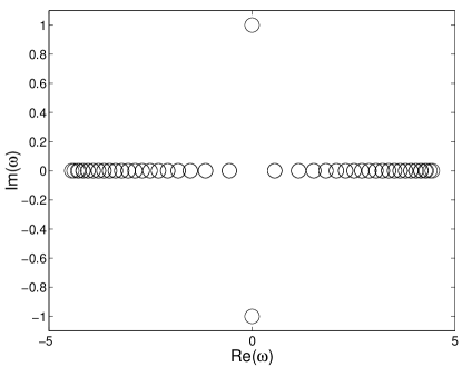
Figure 1: Left panel: Spatial profile of an exact discrete peakon ($a=1$).
Right panel: Spectral plane (Re($\omega$),Im($\omega$)) of the stability matrix for this solution in a Klein–Gordon chain.

This fact can be observed in more detail in Fig. 2, where the dependence of the imaginary part of the unstable eigenvalue of the stability matrix is shown as a function of $a$. This figure also gives the dependence of the energy of the peakon on $a$, which can be analytically calculated: $E(a)=A^{2}\coth(a)/(2a)$. From these figures, it can be deduced that the solution becomes less unstable with (increasing) $a$, or, in other words, when the width of the peakon decreases. This can be equivalently interpreted as a weaker instability as the solution approaches its anti-continuum limit, single-site peakon sibling. This is a rather natural feature of spatial discreteness which typically serves to stabilize coherent structures that are unstable in the continuum limit (e.g., due to collapse) or even ones that do not exist in that limit review .

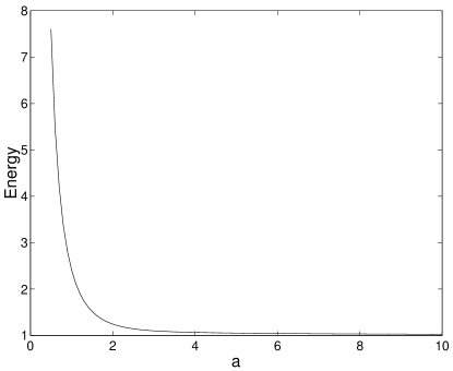
Figure 2: Left panel: Dependence of the maximum imaginary eigenfrequency (i.e., maximum real eigenvalue) of the stability matrix on $a$.
Right panel: Dependence of the energy of the peakon on $a$.

In order to examine the dynamical evolution of the instability of the KG lattice peakon, we used direct numerical simulations, performed with a 5th order Calvo’s symplectic integrator SanzSerna with a time step $\Delta t=0.001$, which preserves the energy up to a factor $10^{-15}$. We introduce a perturbation $\xi_{n}=\varepsilon\pi_{n}$ (to the exact peakon solution $\pi_{n}$) with $\varepsilon=0.1$ to excite the unstable eigendirection. The exponential growth of the peakon instability is shown in the left panel of Fig. 3. If the perturbation were $\xi_{n}=-\varepsilon\pi_{n}$ with $\varepsilon=0.1$ again, the peakon does not grow. Instead, it evolves to a breathing state (see e.g. right panel of Fig. 3), which will be analyzed in Section V.

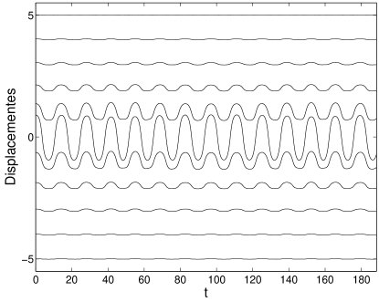
Figure 3: Left panel: Instability evolution of a discrete peakon at different times ($a=1$). Exponential growth can be observed, while the energy of the system is preserved up to a $10^{-15}$ precision. The different snapshots of the solution correspond (from inner to outer) to times 0, 1.8, 2.7 and 3.6.
Right panel: Time evolution of a perturbed peakon that develops into a breathing state. The displacement of the central sites of the peakon are shown as a function of time.

III.3 DNLS 1-site peakons

As explained above, the (spatial dependence of the) profile of a DNLS peakon is the same as that of its Klein-Gordon analog (see Fig. 1). However, in the DNLS setting, the peakon is stable for all values of $a$. This fact has its origin in the gauge invariance of the solutions of DNLS-type equations. In particular, an interesting feature of the discrete peakons is that the $U(1)$ symmetry of the DNLS chain prohibits the single negative energy direction that was present in the KG lattice. Essentially, the unstable direction of the KG lattice is transversal to the same-charge hypersurface in the DNLS case. As a result, perturbations along this potentially unstable direction are banned by the presence of the extra symmetry.

Figure 4 shows the spectral plane for a typical case together with the dependence on $a$ of the charge (also referred to as power in optics) of the peakon. The charge is defined as $Q(u)=\sum_{n}|u_{n}|^{2}/2$ and it can be observed that its value decreases with $a$ and tends to $Q=1/2$ (as should be expected as $a\rightarrow\infty$). This dependence can be analytically calculated: $Q(a)=A^{2}\coth(a)/2$.

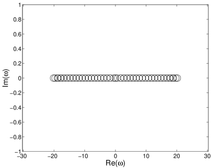
Figure 4: Left panel: Spectral plane of the stability matrix for the peakon of Fig. 1 in the case of the DNLS chain.
Right panel: Dependence of the peakon charge (power) $Q=\sum_{n}\pi_{n}^{2}/2$ as a function of $a$.

The stability of the solution can be verified in the time evolution numerical experiment shown in Fig. 5, which has been performed through a 4th order Runge-Kutta integrator with time step $\Delta t=0.01$. The phase space plot at the central site shows that a randomly perturbed solution remains orbitally close to the exact discrete peakon solution.

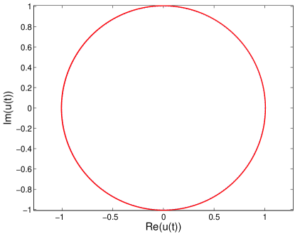
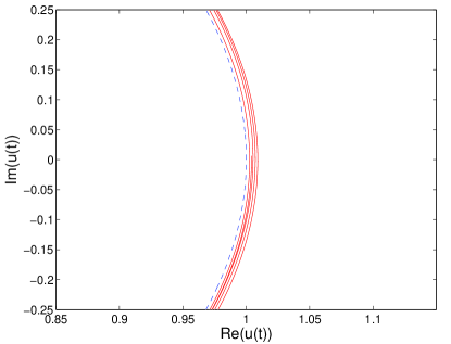
Figure 5: Left panel: Phase space diagram of the central site of a perturbed (full line) and an unperturbed (dashed line) DNLS peakon.
Right panel: A blow-up of the left panel that illustrates the orbital stability of the peakon solution (since the perturbed solution remains in its vicinity).

III.4 2-site Peakons

We now examine the behavior of two-site (i.e., inter-site) peakons, both in the KG, as well as in the DNLS chain.

The energy and charge of 2-site peakons can be analytically calculated as $E(a)=B^{2}/(4a\sinh(a))$ and $Q(a)=B^{2}/(2\sinh(a))$.

Contrary to their single site counterparts, two-site solutions are unstable (also in the DNLS model). In this case, two negative energy directions and hence two imaginary eigenfrequencies could be identified in the spectral plane of the linearization eigenfrequencies in the case of the KG lattice, while one such eigenfrequency was present in the DNLS setting (see Fig. 6). The eigenmode corresponding to the KG case is antisymmetric.

We also simulated the dynamical development of these instabilities, observing that KG two-site peakons are completely destroyed (as their one-site counterparts are also not stable). For the two-site DNLS peakons excited with the perturbation $\epsilon\delta_{n,0}$ with $\epsilon\sim 10^{-4}$, the solution oscillates between the one-site and two-site peakons. These results are shown on Fig. 7.

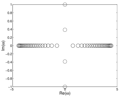
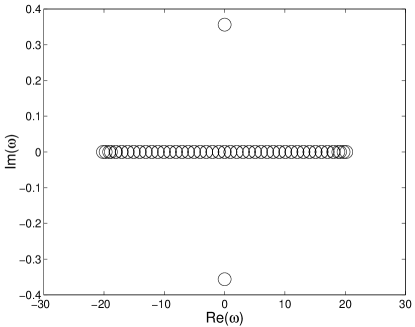
Figure 6: Spectral plane of a the two-site peakon (with $a=1$).
Left panel: KG peakon.
Right panel: DNLS peakon.

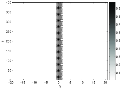
Figure 7: Time evolution of the two-site peakon in the DNLS chain (with $a=1$) induced by perturbing the central particle.
Left panel: The full line represents $|u_{0}|^{2}$, the dashed line represents $|u_{1}|^{2}$.
Right panel: Charge density in space-time.

IV Analytical Results

The above results motivate us to examine the stability of the Klein-Gordon and DNLS peakons from an analytical perspective and, in particular, using energetic considerations. We now proceed to study the stability of the uniform steady state (“vacuum”) and of one-site peakons in each of these settings. The conclusions about stability or instability do not depend on the values of $A$ and $a$, so we set

$$A=1,\qquad a=1,$$

so that the peakon profile is given by

$$\pi_{n}=\exp(-|n|).$$

IV.1 Klein-Gordon

IV.1.1 Hamiltonian formulation.

We can rewrite the Klein-Gordon equation (11) as

$$\ddot{u}_{n}+\partial_{u_{n}}T(u)+\partial_{u_{n}}W(u)=0$$ (18)

where

$$T(u)=-\frac{1}{2}\sum_{(n,m)\in{\mathbb{Z}}^{2}}e^{-|n-m|}u_{n}u_{m},$$ (19)

$$W(u)=\sum_{n\in{\mathbb{Z}}}\left(\left(\frac{\Lambda}{2}+\frac{1}{4}\right)u_{n}^{2}-\frac{1}{4}u_{n}^{2}\ln u_{n}^{2}\right).$$ (20)

Above, $\Lambda$ is a positive constant taken to be

$$\Lambda=(\pi,\pi)=\sum_{n\in{\mathbb{Z}}}e^{-2|n|}=\frac{e^{2}+1}{e^{2}-1},$$ (21)

where $(u,u)=\sum_{n\in{\mathbb{Z}}}u_{n}^{\star}u_{n}$ (in the Klein-Gordon case, we assume that the components $u_{n}$ are real-valued).

Remark 1

Later we will show that the Klein-Gordon equation (18) is globally well-posed in $l^{2}({\mathbb{Z}})\times l^{2}({\mathbb{Z}})$: if both $u(0)$ and $\dot{u}(0)$ belong to $l^{2}({\mathbb{Z}})$, then there is a global solution $u(t)$ with $\|u(t)\|_{l^{2}}<\infty$, $\|\dot{u}(t)\|_{l^{2}}<\infty$ for $0\leq t<\infty$. See Theorem 4. At the same time, the norms $\|u(t)\|_{l^{2}}$, $\|\dot{u}(t)\|_{l^{2}}$ could grow unboundedly large with time.

We can rewrite (18) as

$$\ddot{u}+T^{\prime}(u)+W^{\prime}(u)=0,$$ (22)

where $T^{\prime}(u)$, $W^{\prime}(u)$ may be interpreted as variational derivatives with respect to $u$ of the functionals $T$ and $W$.

The value of the energy functional

$$E_{KG}(u,\dot{u})=\sum_{n\in{\mathbb{Z}}}\frac{\dot{u}_{n}^{2}}{2}+T(u)+W(u)$$ (23)

is conserved along the trajectories of (22).

IV.1.2 Stability of vacuum.

First, let us notice that the zero solution is stable with respect to $l^{2}$-perturbations of the initial data. We bound $T(u)$ by

$$|T(u)|\leq\frac{1}{2}\left|\sup_{n}\sum_{m\in{\mathbb{Z}}}e^{-|n-m|}\right|(u,u)\leq\frac{1}{2}\frac{e+1}{e-1}(u,u).$$ (24)

This inequality is due to the Schur test applied to the matrix $J_{nm}=e^{-|n-m|}$, which yields

$$\|Ju\|_{l^{2}}\leq\left(\sup_{n\in{\mathbb{Z}}}\sum_{m\in{\mathbb{Z}}}|J_{nm}|\right)^{\frac{1}{2}}\left(\sup_{m\in{\mathbb{Z}}}\sum_{n\in{\mathbb{Z}}}|J_{nm}|\right)^{\frac{1}{2}}\|u\|_{l^{2}}=\frac{e+1}{e-1}\|u\|_{l^{2}}.$$ (25)

In the expression (20) for $W(u)$, the first term is $(\frac{\Lambda}{2}+\frac{1}{4})(u,u)$. When the amplitude of $u$ is small, the main contribution in (20) comes from the last term and is of positive sign; thus, for $\|u\|_{l^{\infty}}\equiv\sup_{m}|u_{m}|\leq\epsilon$,

$$E_{KG}(u)\geq\left(-\frac{e+1}{2(e-1)}+\frac{\Lambda}{2}+\frac{1}{4}\right)(u,u)+\frac{1}{4}(u,u)\ln\frac{1}{\epsilon^{2}},$$ (26)

which is positive for $\epsilon$ sufficiently small. Thus, the zero solution minimizes the value of the energy functional among perturbations with bounded amplitude. Since

$$\|u\|_{l^{\infty}}=\sup_{n\in{\mathbb{Z}}}|u_{n}|\leq\left(\sum_{n\in{\mathbb{Z}}}|u_{n}|^{2}\right)^{1/2}=\|u\|_{l^{2}},$$ (27)

the zero solution also minimizes the energy among all perturbations with sufficiently small $l^{2}$-norm.

IV.1.3 Instability of one-site peakons.

Now we address the stability of the peakon $\pi_{n}=e^{-|n|}$. Following Derrick all , let us consider the family of vectors $\pi^{(\lambda)}$ with the components $\pi_{n}^{(\lambda)}=\lambda^{1/2}\pi_{n}$, where $\pi_{n}$ is the peakon profile. We have:

$$E_{KG}(\pi^{(\lambda)})=T(\pi^{(\lambda)})+W(\pi^{(\lambda)})=a\lambda-b\lambda\ln\lambda,$$ (28)

with $a=T(\pi)+W(\pi)$ and $b=\frac{1}{4}\sum_{n\in{\mathbb{Z}}}\pi_{n}^{2}>0$.

Since $\pi$ is a stationary solution to (22), so that

$$T^{\prime}(\pi)+W^{\prime}(\pi)=0,$$ (29)

we have:

$$\frac{d}{d\lambda}\biggr{|}_{{}_{\lambda=1}}T(\pi^{(\lambda)})+W(\pi^{(\lambda)})=(a-b(\ln\lambda+1))\biggr{|}_{{}_{\lambda=1}}=a-b=0,$$ (30)

$$\frac{d^{2}}{d\lambda^{2}}\biggr{|}_{{}_{\lambda=1}}T(\pi^{(\lambda)})+W(\pi^{(\lambda)})=-\frac{b}{\lambda}\biggr{|}_{{}_{\lambda=1}}=-b<0,$$ (31)

thus the stationary solution $\pi$ does not minimize the energy.

It is also easy to check directly that perturbations in the direction of the vector $\frac{d}{d\lambda}\big{|}_{\lambda=1}\pi^{(\lambda)}=\frac{1}{2}\pi$ are linearly unstable. For this, let us consider the solution of the form $\pi_{n}+r_{n}(t)$; the linearized equation on $r$ is

$$\ddot{r}_{n}+\sum_{m\in{\mathbb{Z}}}(T^{\prime\prime}(\pi)+W^{\prime\prime}(\pi))_{nm}r_{m}=0,$$

where $(T^{\prime\prime}(\pi)+W^{\prime\prime}(\pi))_{nm}=\frac{\partial^{2}(T+W)}{\partial u_{n}\partial u_{m}}(\pi)$. The matrix $T^{\prime\prime}(\pi)+W^{\prime\prime}(\pi)$ has the eigenvalue $-1$, with the corresponding eigenvector being $\pi$ itself:

$$\sum_{m\in{\mathbb{Z}}}(T^{\prime\prime}(\pi)+W^{\prime\prime}(\pi))_{nm}\pi_{m}=-\pi_{n}.$$

The perturbation in this direction will grow exponentially, in accordance with our numerical results (cf. Figs. 1-3).

According to shatah-strauss , the linear instability in this model gives rise to the dynamic, or nonlinear, instability:

Theorem 1

The stationary peakon solution $u(t)=\pi$ to (22) is unstable with respect to $l^{2}$-perturbations of the initial data.

IV.2 DNLS

IV.2.1 Hamiltonian formulation.

We now turn to the DNLS equation (12), which can be rewritten as:

$$i\dot{u}_{n}=2\partial_{u^{\star}_{n}}E(u,u^{\star}),$$ (32)

where $E(u,u^{\star})=T(u,u^{\star})+V(u,u^{\star})$, with

$$T(u,u^{\star})=-\frac{1}{2}\sum_{(n,m)\in{\mathbb{Z}}^{2}}e^{-|n-m|}u^{\star}_{n}u_{m},$$ (33)

$$V(u,u^{\star})=\sum_{n\in{\mathbb{Z}}}\left(\left(\frac{\Lambda}{2}-\frac{1}{4}\right)|u_{n}|^{2}-\frac{1}{4}|u_{n}|^{2}\ln|u_{n}|^{2}\right).$$ (34)

The value of the energy functional

$$E(u,u^{\star})=T(u,u^{\star})+V(u,u^{\star})$$

is conserved along the trajectories of (32). The value of the charge functional

$$Q(u,u^{\star})=\frac{1}{2}\sum_{n\in{\mathbb{Z}}}u_{n}u^{\star}_{n}=\frac{1}{2}(u,u)$$

is also conserved (due to the $U(1)$-invariance of the system).

IV.2.2 Stability of vacuum.

Stability of the vacuum solution $u=0$ with respect to $l^{2}$-perturbations of the initial data is proved in the same way as in the case of Klein-Gordon equation: The solution $u=0$ delivers the smallest (zero) value to the energy functional among all vectors $\psi$ of sufficiently small $l^{2}$-norm.

IV.2.3 Stability of one-site DNLS peakons.

In the case of DNLS, the perturbation $u\mapsto u+\epsilon u$ would lead to smaller values of the energy functional as in the case of Klein-Gordon equation. However, now this perturbation is prohibited by the charge conservation. Therefore, we expect that the peakons are local minimizers of the energy functional under the charge constraint and hence are orbitally stable.

We will prove the following theorem:

Theorem 2

The standing wave solution $e^{it}\pi$ to (12) is orbitally stable with respect to $l^{2}$-perturbations of the initial data.

Let us remind the definition of the orbital stability (see strauss ):

Definition 1

The $\pi$-orbit $\{e^{is}\pi{\rm;}\ s\in{\mathbb{R}}\}$ is stable if for all $\varepsilon>0$ there exists $\delta>0$ with the following property. If $u_{0}\in l^{2}({\mathbb{Z}},{\mathbb{C}})$ is such that $\|u_{0}-\pi\|_{l^{2}}<\delta$ and $u(t)$ is a solution of Eq. (12) in some interval $[0,t_{1})$, then $u(t)$ can be continued to a solution in $0\leq t<\infty$ and

$$\sup_{0<t<\infty}\inf_{s\in{\mathbb{R}}}\|u(t)-e^{is}\pi\|_{l^{2}}<\varepsilon.$$

Otherwise the $\pi$-orbit is called unstable.

Remark 2

Eq. (12) is locally well-posed in $l^{2}({\mathbb{Z}},{\mathbb{C}})$ since for $u\in l^{2}$ the right-hand side of (12) (where we set $A=1$, $a=1$) is also in $l^{2}$:

$$\left\|-\sum_{m\in{\mathbb{Z}}}J_{nm}u_{m}+\left[\frac{2}{e^{2}-1}-\frac{1}{2}\ln\left(u_{n}u_{n}^{\star}\right)\right]u_{n}\right\|_{l^{2}}\leq\left[\frac{e+1}{e-1}+\frac{2}{e^{2}-1}+\left|\ln\|u\|_{l^{2}}\right|\right]\|u\|_{l^{2}}.$$ (35)

We used inequalities (25) and (27). Hence, for any $u_{0}\in l^{2}({\mathbb{Z}},{\mathbb{C}})$, there exists $\tau>0$ so that there is a unique solution $u(t)$ defined for $0\leq t<\tau$ that satisfies $u(0)=u_{0}$. Due to the conservation of the charge $Q(u)=\|u\|_{l^{2}}^{2}/2$ along the flow of Eq. (12), we conclude that $u(t)$ is defined globally: $u\in C^{1}([0,\infty),l^{2}({\mathbb{Z}},{\mathbb{C}}))$. This settles the question about the global well-posedness for (12) in $l^{2}({\mathbb{Z}},{\mathbb{C}})$ which is a necessary condition for the orbital stability.

According to strauss , we will know the orbital stability of the peakon if we can prove that $H=E^{\prime\prime}(\pi)+Q^{\prime\prime}(\pi)$ defines a quadratic form that is positive-definite on vectors that are tangent to the hypersurface of the same charge and are orthogonal to the orbit spanned by $\pi$.

Remark 3

Once one knows that $H$ defines a positive-definite quadratic form on vectors tangent to same charge hypersurface and orthogonal to the orbit of $\pi$, one proves that there exist $\delta>0$ and $C>0$ such that for any $u$ with $Q(u)=Q(\pi)$ and $\|u-\pi\|_{l^{2}}<\delta$ one has $E(u)-E(\pi)\geq C\inf_{s}\|u-e^{is}\pi\|_{l^{2}}$ (Theorem 3.4 in strauss ) and then the orbital stability follows from Theorem 3.5 in strauss .

We will use the real-valued formulation. For $u(t)=v(t)+iw(t)\in l^{2}({\mathbb{Z}},{\mathbb{C}})$, with $v=\{v_{n}\}$, $w=\{w_{n}\}$ real-valued, we write

$$\bm{u}(t)=\left[\begin{array}[]{c}v(t)\\ w(t)\end{array}\right],\qquad\bm{u}(t)\in l^{2}({\mathbb{Z}},{\mathbb{R}}^{2}).$$

The equation on $\bm{u}$ is

$$\dot{\bm{u}}=JE^{\prime}(\bm{u})=\left[\begin{array}[]{cc}0&1\\ -1&0\end{array}\right]\left[\begin{array}[]{c}\nabla_{v}E\\ \nabla_{w}E\end{array}\right],$$

and the stationary equation on $\bm{\pi}=\left[\begin{array}[]{c}\pi\\ 0\end{array}\right]$ is given by

$$E^{\prime}(\bm{\pi})+Q^{\prime}(\bm{\pi})=0.$$

Let $\psi=\xi+i\eta,$ $\bm{\psi}=\left[\begin{array}[]{c}\xi\\ \eta\end{array}\right].$ The vectors tangent to the same charge hypersurface satisfy

$$\langle Q^{\prime}(\bm{\pi}),\bm{\psi}\rangle=\langle\bm{\pi},\bm{\psi}\rangle=\sum_{n\in{\mathbb{Z}}}\pi_{n}\xi_{n}=0,$$ (36)

while the vectors orthogonal to $\left[\begin{array}[]{c}0\\ \pi\end{array}\right]=-J\bm{\pi}$ (this vector corresponds to $i\pi$, a tangent direction to the orbit spanned by $e^{it}\pi$) satisfy

$$\langle-J\bm{\pi},\bm{\psi}\rangle=-\sum_{n\in{\mathbb{Z}}}\pi_{n}\eta_{n}=0.$$ (37)

As we mentioned in Remark 3, Theorem 2 will be proved if we can show that the quadratic form defined by the Hamiltonian operator

$$H=E^{\prime\prime}(\bm{\pi})+Q^{\prime\prime}(\bm{\pi})$$

is positive-definite on vectors $\bm{\psi}=\left[\begin{array}[]{c}\xi\\ \eta\end{array}\right]$, where both $\xi$ and $\eta$ are orthogonal to $\pi$.

Let us find the explicit expression for $H$. For the second Fréchet derivative of $T$, we compute:

$$\langle T^{\prime\prime}(\bm{\pi})\bm{\psi},\bm{\psi}\rangle=-\sum_{(n,m)\in{\mathbb{Z}}^{2}}e^{-|n-m|}\left(\xi_{n}\xi_{m}+\eta_{n}\eta_{m}\right).$$ (38)

For the “potential” term, we compute

$$\langle V^{\prime\prime}(\bm{\pi})\bm{\psi},\bm{\psi}\rangle=\sum_{n\in{\mathbb{Z}}}\left((\Lambda-1)(\xi^{2}_{n}+\eta^{2}_{n})+|n|(\xi^{2}_{n}+\eta^{2}_{n})-\xi^{2}_{n}\right).$$ (39)

For the charge functional, we have

$$\langle Q^{\prime\prime}(\bm{\pi})\bm{\psi},\bm{\psi}\rangle=\sum_{n\in{\mathbb{Z}}}\left(\xi^{2}_{n}+\eta^{2}_{n}\right).$$ (40)

Hence, the operator $H=E^{\prime\prime}(\bm{\pi})+Q^{\prime\prime}(\bm{\pi})=T^{\prime\prime}(\bm{\pi})+V^{\prime\prime}(\bm{\pi})+Q^{\prime\prime}(\bm{\pi})$ is given by

$$\langle H\bm{\psi},\bm{\psi}\rangle =-\sum_{(n,m)\in{\mathbb{Z}}^{2}}e^{-|n-m|}\left(\xi_{n}\xi_{m}+\eta_{n}\eta_{m}\right)$$

$$\quad\qquad+\sum_{n\in{\mathbb{Z}}}\left(\left(\Lambda-1+|n|\right)(\xi^{2}_{n}+\eta^{2}_{n})+\eta^{2}_{n}\right).$$

We have:

$$\langle H\bm{\psi},\bm{\psi}\rangle=\left[\xi,\eta\right]\left[\begin{array}[]{cc}H^{+}&0\\ 0&H^{-}\end{array}\right]\left[\begin{array}[]{c}\xi\\ \eta\end{array}\right],$$ (42)

where

$$H^{+}_{nm}=-e^{-|n-m|}+\left(\Lambda-1+|n|\right)\delta_{nm}$$ (43)

$$H^{-}_{nm}=-e^{-|n-m|}+\left(\Lambda+|n|\right)\delta_{nm}.$$ (44)

Let us consider the symmetric matrix

$$A_{nm}=-e^{-|n-m|}+|n|\delta_{nm}+\pi_{n}\pi_{m}.$$ (45)

Numerical computations show that this matrix does not have negative eigenvalues and that the dimension of its null space is $\dim N(A)=3$. One can check that $N(A)$ is spanned by the vectors $v^{(+)}$, $v^{(-)}$, and $v^{(0)}$:

$$v^{(+)}_{n}=\theta(n+1/2)e^{-|n|},$$

$$v^{(-)}_{n}=v^{(+)}_{-n}=\theta(-n+1/2)e^{-|n|},$$

$$v^{(0)}_{n}=\delta_{n,0}$$

where $\theta(n)=1$ for $n>0$ and $0$ for $n<0$. In particular,

$$\pi=v^{(+)}+v^{(-)}-v^{(0)}\in N(A).$$

Since $A$ is symmetric, the eigenvectors that correspond to other (positive) eigenvalues of $A$ are orthogonal to $\pi$.

The matrices $H_{nm}^{+}$, $H_{nm}^{-}$ can be expressed as

$$H_{nm}^{+}=A_{nm}-\pi_{n}\pi_{m}+(\Lambda-1)\delta_{nm},$$ (46)

$$H_{nm}^{-}=A_{nm}-\pi_{n}\pi_{m}+\Lambda\delta_{nm}=H_{nm}^{+}+\delta_{nm}.$$ (47)

We have: $H^{+}\pi=A\pi-(\pi,\pi)\pi+(\Lambda-1)\pi=-\pi$, since $(\pi,\pi)=\Lambda$, and $H^{-}\pi=0$. Since $H^{+}$ and $H^{-}$ are symmetric, their other eigenvectors are orthogonal to $\pi$. But then they also have to be the eigenvectors of $A$. The corresponding eigenvalues are those of $A$ shifted to the right by $(\pi,\pi)-1>0$ (for $H^{+}$) and by $(\pi,\pi)$ (for $H^{-}$), and hence are strictly positive.

Remark 4

The important feature of this model that makes the analysis simple is that $H^{+}$ and $H^{-}$ can be diagonalized simultaneously.

Thus, assuming that $\psi=\xi+i\eta\in l^{2}({\mathbb{Z}},{\mathbb{C}})$ satisfies (36) and (37) (both $\xi$ and $\eta$ are orthogonal to $\pi$) and is different from zero, we conclude that $\langle H\bm{\psi},\bm{\psi}\rangle$ is positive-definite:

$$\langle H\bm{\psi},\bm{\psi}\rangle=\sum_{(n,m)\in{\mathbb{Z}}^{2}}\left(H^{+}_{nm}\xi_{n}\xi_{m}+H^{-}_{nm}\eta_{n}\eta_{m}\right)>0$$

and hence the one-site peakon solutions are dynamically stable.

IV.2.4 Two-site DNLS peakons

One can also prove the following theorem:

Theorem 3

The 2-site standing wave solution to (12) is orbitally unstable with respect to $l^{2}$-perturbations of the initial data.

The generalization of the matrices $H^{+}$ and $H^{-}$ given above in Eq. (43) and (44) is given by:

$$H^{+}_{nm}=-e^{-|n-m|}+\left(\Lambda-1-\ln(u_{n})\right)\delta_{nm}$$ (48)

$$H^{-}_{nm}=-e^{-|n-m|}+\left(\Lambda+\ln(u_{n})\right)\delta_{nm}.$$ (49)

In the case of the inter-site solution, known explicitly as

$$u_{n}=\frac{1}{2}\frac{(e-1)}{e+1}e^{it}e^{-|n-1/2|},$$ (50)

the eigenvalues of $H^{+}$, $H^{-}$ can be explicitly computed. As expected, $u_{n}$ is itself an eigenvector with eigenvalue $-1$ (see above), while the second eigenvalue is $\lambda_{2}=-0.149$. However, since the eigenvalues of $H^{-}$ are the ones of $H^{+}$ shifted by $1$, this results in $n(H^{+})-n(H^{-})=2$, where $n(H^{\pm})$ denotes the number of negative eigenvalues of the matrices $H^{\pm}$. From the theory of strauss ; jones ; grillakis (see also the recent work of kapitula ; pelinovsky ), this implies that there is one real eigenvalue in the spectrum of linearization of the DNLS 2-site peakon, in agreement with our numerical observations of Section III. This completes the proof of Theorem 3.

V Breathing peakons in the discrete Klein-Gordon equation

V.1 Existence of Breathing Peakons

We are interested in solutions to the Klein-Gordon equation (18) that have the form

$$u_{n}(t)=g(t)f_{n},$$ (51)

where $g(t)$ is a scalar-valued function.

Trying the peakon profile, $f=\pi$, so that $u_{n}(t)=g(t)e^{-|n|}$, we get the following equation on $g(t)$:

$$\ddot{g}=\frac{1}{2}g\ln g^{2},\qquad g=g(t).$$ (52)

We can integrate Eq. (52), getting

$$\frac{\dot{g}^{2}}{2}+\frac{g^{2}}{4}(1-\ln g^{2})={\mathcal{E}},$$ (53)

where ${\mathcal{E}}\geq 0$ is the “energy of breathing”. The function ${\mathcal{V}}(g)=\frac{g^{2}}{4}(1-\ln g^{2})$ (see Fig. 8) represents the potential in which $g$ lives.

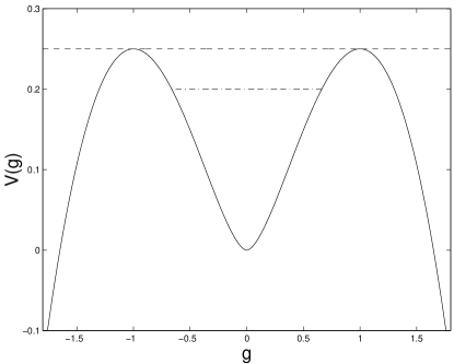
Figure 8: Potential ${\mathcal{V}}(g)$. The (unstable) stationary solutions $g=\pm 1$ correspond to the (unstable) peakons, $u(t)=g(t)\pi=\pm\pi$, while the (stable) stationary solution $g=0$ corresponds to the vacuum (which we know to be stable). There are also oscillating solutions that correspond to breathing oscillations with the energy ${\mathcal{E}}$, $0\leq{\mathcal{E}}<1/4$. A breathing “bound state” at ${\mathcal{E}}=0.2$ is also shown by dash-dotted line.

V.2 Global well-posedness for the discrete Klein-Gordon equation in $l^{2}\times l^{2}$

Before analyzing the stability of the breathing peakons, we need to consider the initial value problem for the equation of the Klein-Gordon lattice (18).

Theorem 4

Eq. (18) is globally well-posed in $l^{2}\times l^{2}$. That is, for any initial data $(u_{0},v_{0})\in l^{2}({\mathbb{Z}})\times l^{2}({\mathbb{Z}})$, there is a unique solution $u(t)$ that satisfies $u(0)=u_{0}$, $\dot{u}(0)=v_{0}$; this solution is defined for all times $t\geq 0$, and moreover $\|u(t)\|_{l^{2}}+\|\dot{u}(t)\|_{l^{2}}$ remains finite for all $t\geq 0$:

$$u\in C^{2}([0,\infty),l^{2}({\mathbb{Z}})).$$

Let us first discuss the local well-posedness of (18) in $l^{2}$. We claim that for any $(u_{0},v_{0})\in l^{2}({\mathbb{Z}})\times l^{2}({\mathbb{Z}})$, there exists $\tau>0$ such that there is a unique solution $u(t)$ defined for $0\leq t<\tau$ with $(u,\dot{u})=(u_{0},v_{0})$ and $u\in C^{1}([0,\tau),l^{2}({\mathbb{Z}}))$. This claim immediately follows from the observation that if $u\in l^{2}({\mathbb{Z}})$, then $\ddot{u}$ given by (18) is also from $l^{2}({\mathbb{Z}})$. This is verified as in (35).

Now we turn to the global well-posedness. Let us prove the boundedness of $L(t)=\|u(t)\|_{l^{2}}^{2}$. Let us derive the equation for $d^{2}L(t)/dt^{2}$. We have:

$$\frac{d^{2}}{dt^{2}}L(t)=2(\dot{u},\dot{u})+2(u,\ddot{u}).$$

The total energy $\frac{1}{2}(\dot{u},\dot{u})+T(u)+W(u)$ is conserved along the flow generated by (18) allowing to express

$$(\dot{u},\dot{u})=2E_{0}-2T(u)-2W(u),$$ (54)

where $E_{0}=(v_{0},v_{0})/2+T(u_{0})+W(u_{0})$ and $(u_{0},v_{0})$ is the initial data that corresponds to the solution $u(t)$.

Thus, we obtain:

$$\frac{d^{2}}{dt^{2}}L(t) = 4E_{0}-4T(u)-4W(u)-2(u,\partial_{u}T)-2(u,\partial_{u}W)$$

$$= 4E_{0}-8T(u)+\sum_{n\in{\mathbb{Z}}}\left(-\left(4\Lambda+1\right)u_{n}^{2}+2u_{n}^{2}\ln u_{n}^{2}\right).$$

Using the straightforward bounds on the terms in the right-hand side, namely

$$-T(u)\leq\frac{e+1}{2(e-1)}L$$ (55)

that follows from (24), and also

$$\sum_{n\in{\mathbb{Z}}}u_{n}^{2}\ln u_{n}^{2}\leq\sum_{n\in{\mathbb{Z}}}u_{n}^{2}\ln\|u\|_{l^{\infty}}^{2}\leq\sum_{n\in{\mathbb{Z}}}u_{n}^{2}\ln L=L\ln L,$$ (56)

where in the second inequality we used relation (27), we conclude that, for some $C=C(E_{0})>0$,

$$\frac{d^{2}}{dt^{2}}L\leq C(1+L+2L\ln L).$$ (57)

For $L\geq 1$, the right-hand side is monotonically increasing (and exceeds its range for $0<L<1$). Therefore, $0\leq L(t)\leq Z(t)$, where $Z(t)$ is a function that satisfies

$$Z^{\prime\prime}(t)=C(1+Z+2Z\ln Z)$$ (58)

and the initial data

$$Z(0)=\max(1,L(0))=\max(1,(u_{0},u_{0})),$$

$$Z^{\prime}(0)=\max\left(1,\frac{dL}{dt}\biggr{|}_{{}_{t=0}}\right)=\max\left(1,2(u_{0},v_{0})\right).$$

We can rewrite (58) as

$$Z^{\prime\prime}+C\partial_{Z}(-Z-Z^{2}\ln Z)=0;$$ (59)

multiplying by $Z^{\prime}$ and integrating in $t$, we get

$$\frac{(Z^{\prime})^{2}}{2}-CZ-CZ^{2}\ln Z=E,$$

where $E=\frac{(Z^{\prime}(0))^{2}}{2}+C(-Z(0)-Z^{2}(0)\ln Z(0))$ is a constant of integration. Expressing $Z^{\prime}$ and separating variables, we get

$$t=\int_{Z(0)}^{Z(t)}\frac{dZ}{\sqrt{E+CZ+CZ^{2}\ln Z}}.$$

Since the integral $\int_{Z(0)}^{\infty}\frac{dZ}{\sqrt{E+CZ+CZ^{2}\ln Z}}$ diverges at the upper limit (as $\ln^{\frac{1}{2}}Z$), we conclude that $Z$ can not become infinite in finite time.

The finiteness of $l^{2}$-norm of $\dot{u}$ follows from relation (54), bounds (55) and (56), and the finiteness of $L=\|u\|_{l^{2}}^{2}$ that we already proved.

This finishes the proof of Theorem 4.

V.3 Linearized stability of Breathing Peakons

We will now analyze the linear stability of the breathing peakon, showing the absence of the exponential instability of small perturbations of the initial data. We rewrite Eq. (18) as the first order system,

$$\left\{\begin{array}[]{l}\dot{u}=v\\ \dot{v}=-\partial_{u}(T(u)+W(u)),\end{array}\right.$$ (60)

and consider the perturbation of the solution $(u_{0}(t),v_{0}(t))=(g(t)\pi,\dot{g}(t)\pi)$ that corresponds to the peakon:

$$u(t)=u_{0}(t+\gamma(t))+\delta u(t),\qquad v(t)=v_{0}(t+\gamma(t))+\delta v(t).$$

The function $\gamma(t)$ adjusts the location of the breather $(g(t)\pi,\dot{g}(t)\pi)$ so that it is closer (in a certain sense) to the perturbed solution $(u(t),v(t))$. We consider the linearization of system (60). For this, we first compute

$$T^{\prime\prime}(g\pi)+W^{\prime\prime}(g\pi)=T^{\prime\prime}(\pi)+W^{\prime\prime}(\pi)-\frac{\ln g^{2}}{2}=H^{+}-\frac{\ln g^{2}}{2},$$ (61)

where $H^{+}$ was introduced in (46), and then we can write

$$\left\{\begin{array}[]{l}g^{\prime}(t+\gamma(t))\dot{\gamma}(t)\pi+\partial_{t}\delta u(t)=\delta v(t),\\ g^{\prime\prime}(t+\gamma(t))\dot{\gamma}(t)\pi+\partial_{t}\delta v(t)=-(H^{+}-\frac{\ln g^{2}}{2})\delta u(t).\end{array}\right.$$ (62)

We split

$$\delta u(t)=a(t)\pi+\phi(t),\qquad\delta v(t)=b(t)\pi+\psi(t),$$

with $\phi$, $\psi\in l^{2}({\mathbb{Z}})$ both orthogonal to $\pi$. Projecting system (62) onto $\pi$, gives the following system:

$$\left\{\begin{array}[]{l}g^{\prime}(t+\gamma(t))\dot{\gamma}(t)+\dot{a}(t)=b(t),\\ g^{\prime\prime}(t+\gamma(t))\dot{\gamma}(t)\pi+\dot{b}(t)=-(-1-\frac{\ln g^{2}}{2})a(t),\end{array}\right.$$ (63)

where we used the fact that $\pi$ is an eigenvector, $H^{+}\pi=-\pi$. Projection of (62) onto the direction normal to $\pi$ gives the following system:

$$\left\{\begin{array}[]{l}\dot{\phi}(t)=\psi(t),\\ \dot{\psi}(t)=-(H^{+}-\frac{\ln g^{2}}{2})\phi(t).\end{array}\right.$$ (64)

The analysis of system (63) is straightforward. We would arrive at this system if we pursued the stability analysis of Eq. (52). At the same time, we could analyze that equation topologically. It corresponds to an unharmonic oscillator; its phase portrait in the $(g,\dot{g})$ plane contains a set of closed trajectories circling around the origin (they correspond to the initial data $(g,\dot{g})$ such that $|g|<1$ and the value of ${\mathcal{E}}$ in (53) is smaller than $1/4$). Each of these closed trajectories is stable with respect to small perturbations of the initial data: There is a neighboring closed trajectory passing through the point that corresponds to the perturbed initial data.

Let us now analyze system (64). We can rewrite it as $\dot{\Phi}={\bf J}{\bf H}\Phi,$ where

$$\Phi=\left[\begin{array}[]{c}\phi\\ \psi\end{array}\right],\quad{\bf J}=\left[\begin{array}[]{cc}0&1\\ -1&0\end{array}\right],\quad{\bf H}=\left[\begin{array}[]{cc}H^{+}-\frac{\ln g^{2}}{2}&0\\ 0&1\end{array}\right],$$

with $\phi$, $\psi$ orthogonal to $\pi$. The matrix $H^{+}$ (see (46) and thereafter) has eigenvalues

$$\sigma(H^{+})=\{-1,\Lambda-1,\dots\},$$

where the only negative eigenvalue $-1$ corresponds to $\pi$ and the next eigenvalue, $\Lambda-1$, is positive. The term $-\frac{\ln g^{2}}{2}$ in (61) further shifts the spectrum upwards as long as $|g|<1$. Therefore, ${\bf H}$ is positive-definite on the space $\pi^{\perp}\times l^{2}({\mathbb{Z}})$. Thus, $\sqrt{{\bf H}}$ is well-defined; the matrix ${\bf J}{\bf H}$ is similar to $\sqrt{{\bf H}}\,{\bf J}\sqrt{{\bf H}}$ and hence has purely imaginary spectrum.

This shows that the breathing peakon solutions $g(t)\pi$ to (18) are spectrally stable.

Remark 5

This linearized approach to the stability does not prove the dynamic orbital stability of the breathing peakons. The nonlinear terms may transfer the energy between “breathing” oscillations in $\pi$-direction and the perturbations in the space $\pi^{\perp}$, pumping the energy from system (63) into (64). It is therefore possible that the energy of the breathing peakon, after a small perturbation, would wind up transferred, partially or completely, into directions orthogonal to $\pi$ (and then maybe back). We do not have a satisfactory description of this process, even though we believe that techniques such as the Hamiltonian dispersive normal forms of SW could be relevant in addressing it. While outside the scope of the present study, this may be an interesting question for future investigations.

V.4 Numerical Results

An orbit of frequency $\omega_{\mathrm{p}}$ for $g(t)$ can be determined by solving Eq. (52). This can be done through a variety of methods such as, e.g., a shooting method in real space or using quadratures. Here we have chosen a Chebyshev quadrature method in order to integrate the equation.

Figure 9 shows the dependence of $g(0)$ and ${\mathcal{E}}$ of the peakon frequency $\omega_{\mathrm{p}}$. It can clearly be observed (see the left end of the graphs) that as $\omega_{\mathrm{p}}\rightarrow 0$, the energy approaches $1/4$ and the amplitude is $1$, hence the solution is very close to the unstable critical point of ${\mathcal{E}}=1/4$ and $g=1$. We can also observe that the peakon frequency can have any value as there do not exist resonances with the continuous spectrum (actually, such small amplitude, extended wave excitations do not exist since ${\mathcal{V}}^{\prime\prime}(0)=\infty$).

Figure 10 shows the time evolution of a breathing peakon. It is worth pointing out that the main difference between DNLS peakons and KG breathing peakons is that, in the first case, only the first Fourier coefficient is different from zero, whereas in the second case, there are more non-zero coefficients.

We have confirmed in the numerical simulations that initial conditions corresponding to a perturbed discrete breathing peakon stays orbitally close to the exact solution. Figure 11 shows the difference between the evolution of the central particle of the peakon in a perturbed and an unperturbed case. The perturbation used is $\xi_{n}=\varepsilon\delta_{n,0}$ with $\varepsilon=0.01$. The perturbed peakon appears to be orbitally stable.

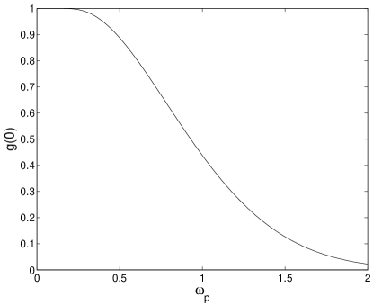
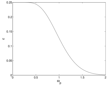
Figure 9: Dependence of $g(0)$ (left) and ${\mathcal{E}}$ with respect to the peakon frequency.

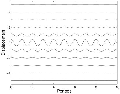
Figure 10: Time evolution of the breathing peakon (the displacement of each of the first few sites is shown as a function of time).

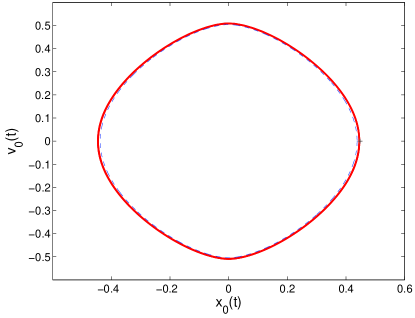
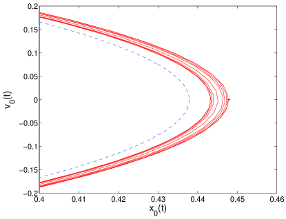
Figure 11: Left panel: Phase space diagram of the central site of a perturbed (full line) and an unperturbed (dashed line) breathing peakon with $\omega_{\mathrm{p}}=1$.
Right panel: Blow-up of the left panel.
The cross indicates the initial point of the simulation.

Contrary to the static case, breathing two-site peakons are not destroyed by perturbations. Instead, the energy density oscillates as shown in Fig. 12.

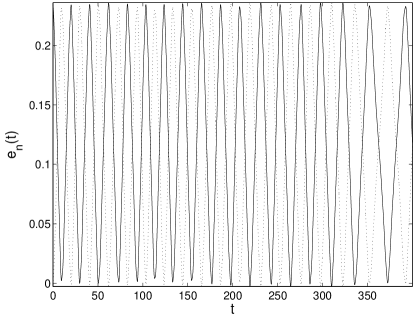
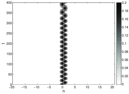
Figure 12: Time evolution of the two-site breathing peakon chain (with $a=1$ and $\omega_{p}=1$) perturbed with the antisymmetric mode.
Left panel: The full line represents $e_{0}$, the dashed line represents $e_{1}$, where $e_{n}$ is the energy density of the $n$-th site.
Right panel: Energy density in the space-time evolution.

VI Discussion

In this paper, we have engineered a mathematical model that has discrete peakons as exact solutions. The continuum version of the model was also given and its ability to support the continuum analog of the solutions was highlighted. Both the dispersive and the nonlinear part of the relevant interactions were connected to earlier works. Furthermore, it was advocated that for suitable choice of the interaction range, this can be a relevant model in nonlinear optics with the characteristic features of photorefractive materials christo , while being a lattice dynamical model of interest in its own right.

We have identified the discrete peakon solutions analogous to their (discontinuous in the first derivative) continuum limit, i.e., $\pi_{n}\sim\exp(-|n|)$, as well as their inter-site siblings. However, a natural question of interest would be whether there is a more general way of defining such solutions in the discrete setting. This is particularly relevant as solutions similar to the ones obtained here have appeared in other contexts. Such examples consist of, e.g., the waveform of Fig. 1 in kovalev (arising from the presence of an impurity) or that of Fig. 7 in gaid6 (arising because of the interplay of nonlinearity with long range interactions, as is the case in this paper). Perhaps, an alternative criterion possibly involving the sign of the second difference close to the center of the wave could be used for a more general definition of the discrete peakon. This would be an interesting topic for future studies.

We have also investigated the stability of such discrete waves and have found discrete peakons to be particularly interesting from this aspect as well. We have numerically observed that in the Klein-Gordon lattice setting such solutions are always unstable; however the negative energy direction responsible for this instability is eliminated due to an additional symmetry (the phase invariance that leads to the $l^{2}$-norm conservation) in the case of the DNLS chain. We showed (using a Derrick-type argument) that the peakon is not a local minimizer of the energy in the Klein-Gordon case and moreover indicated the direction of the perturbation that leads to a linear instability. We also showed that in the $U(1)$-invariant DNLS equation the peakon is a local minimizer of the energy under the charge constraint and hence is orbitally stable. Contrary to their one-site counterparts, two-site peakons proved to be unstable, as was explicitly demonstrated via a well-known functional analytic criterion relevant to DNLS type equations.

Finally, using a separation of variables approach, we were able to show the existence of the exact periodic (breathing) peakon solutions in the Klein-Gordon lattice. The breathing peakons were shown to correspond to the subcritical initial conditions, while supercritical initial conditions lead to the amplitude of the solution tending to infinity (in infinite time), with the unstable static peakon being the separatrix between the two types of behavior. We also systematically tackled the initial value problem for the Klein-Gordon lattice and showed that the finite-time blow-up of the $l^{2}$-norm of the solution is not possible, so that the system is globally well-posed. We then proved the absence of the linear instability of the breathing peakons. Yet, the question of the long-time behavior of perturbed breathing peakons remains open.

It may be interesting to try to extend this class of models to higher dimensional settings and observe how their dynamical behavior is affected by the dimensionality of the underlying lattice.

AC was supported in part by the National Science Foundation grant DMS-0200880 and by the Max Planck Institute, Leipzig. JC acknowledges an FPDI grant from ‘La Junta de Andalucía’ and partial support under the European Commission RTN project LOCNET, HPRN-CT-1999-00163 and the MECD/FEDER project FIS2004-01183. PGK gratefully acknowledges support from NSF-DMS-0204585, the Eppley Foundation for Research and from an NSF-CAREER award. We are thankful to Sergej Flach for bringing Ref. flach to our attention. We are also indebted to an anonymous referee for bringing to our attention a recent paper oster , as well as several earlier relevant works.

References

- (1)
- (2) S. Aubry, Physica 103D, 201 (1997); S. Flach and C.R. Willis, Phys. Rep. 295, 181 (1998); Physica 119D, (1999), special volume edited by S. Flach and R.S. MacKay; focus issue edited by Yu. S. Kivshar and S. Flach, Chaos 13, 586-799 (2003).
- (3) See, e.g., A.A. Sukhorukov et al., IEEE J. Quantum Elect. 39, 31 (2003); U. Peschel et al., J. Opt. Soc. Am. B 19, 2637 (2002).
- (4) A. Trombettoni and A. Smerzi, Phys. Rev. Lett. 86, 2353, (2001); F.Kh. Abdullaev et al., Phys. Rev. A64, 043606 (2001); F.S. Cataliotti et al., Science 293, 843 (2001); A. Smerzi et al., Phys. Rev. Lett. 89, 170402 (2002). G. L. Alfimov, P. G. Kevrekidis, V. V. Konotop, and M. Salerno Phys. Rev. E 66, 046608 (2002).
- (5) E.N. Pelinovsky and S.K. Shavratsky, Physica 3D, 410 (1981).
- (6) P. Binder et al., Phys. Rev. Lett. 84, 745 (2000); E. Trías, J. J. Mazo, and T. P. Orlando, Phys. Rev. Lett. 84, 741 (2000).
- (7) M. Peyrard, and A.R. Bishop, Phys. Rev. Lett., 62, 2755 (1989); T. Dauxois, M. Peyrard and A.R. Bishop, Phys. Rev. E, 47, R44 (1993); T. Dauxois, M. Peyrard and A.R. Bishop, Phys. Rev. E, 47, 684 (1993); M. Peyrard et al., Physica 68D, 104 (1993); A. Campa, and A. Giansanti, Phys. Rev. E, 58, 3585 (1998).
- (8) Y.S. Kivshar and B.A. Malomed Rev. Mod. Phys. 61, 763 (1989).
- (9) P. Rosenau and J.M. Hyman, Phys. Rev. Lett. 70, 564 (1993).
- (10) L.D. Landau and E.M. Lifshitz, Hydrodynamics, 4th ed. (Nauka, Moscow 1988).
- (11) W. Chen and D.L. Mills, Phys. Rev. Lett. 58, 160 (1987).
- (12) P.G. Kevrekidis and V.V. Konotop, Phys. Rev. E 65, 066614 (2002); P.G. Kevrekidis, V.V. Konotop, A.R. Bishop and S. Takeno, J. Phys. A 35, L641-L652 (2002); M. Öster, M. Johansson and A. Eriksson, Phys. Rev. E 67, 056606 (2003).
- (13) V.V. Konotop, Chaos, Solitons and Fractals, 11, 153 (2000).
- (14) A.A. Sukhorukov and Y.S. Kivshar, Opt. Lett. 27, 2112 (2002); P.G. Kevrekidis, B.A. Malomed and Z. Musslimani, Eur. Phys. J. D, 23, 421 (2003); A.V. Gorbach and M. Johansson, Phys. Rev. E 67, 066608 (2003).
- (15) The recent work of M. Öster, Yu.B. Gaididei, M. Johansson and P.L. Christiansen, Physica D 198, 29 (2004) numerically identified discrete peakons in a model with nonlocal and nonlinear dispersion and compared them with quasi-continuous approximations.
- (16) R. Camassa and D.D. Holm, Phys. Rev. Lett. 71, 1661 (1993).
- (17) M.S. Alber, R. Camassa, D.D. Holm and J.E. Marsden, Lett. Math. Phys. 32, 137 (1994).
- (18) A.G. Litvak and A.M. Sergeev, JETP Lett. 27, 517 (1978).
- (19) A.A. Ovchinnikov and S. Flach, Phys. Rev. Lett. 83, 248 (1999).
- (20) P.G. Kevrekidis, K.Ø. Rasmussen and A.R. Bishop, Int. J. Mod. Phys. B 15, 2833 (2001).
- (21) G.A. Baker Jr., Phys. Rev. 122, 1477 (1961).
- (22) A.M. Kac and B.C. Helfand, J. Math. Phys. 4, 1078 (1972).
- (23) S.F. Mingaleev, P.L. Christiansen, Yu.B. Gaididei, M. Johansson and K.Ø. Rasmussen, Jour. Biol. Phys. 25, 41 (1999).
- (24) Yu.B. Gaididei, S.F. Mingaleev and P.L. Christiansen, Phys. Rev. E 62, R53 (2000).
- (25) P.L. Christiansen, Yu.B. Gaididei and S.F. Mingaleev, J. Phys.: Cond. Matt. 13, 1181 (2001).
- (26) S.F. Mingaleev, Yu.B. Gaididei, P.L. Christiansen and Yu.S. Kivshar, Europhys. Lett. 59, 403 (2002).
- (27) S.F. Mingaleev, Yu.B. Gaididei and F.G. Mertens, Phys. Rev. E 58, 3833 (1998).
- (28) P.L. Christiansen, Y.B. Gaididei, F.G. Mertens and S.F. Mingaleev, Eur. Phys. J. B 19, 545 (2001).
- (29) B. Fornberg and G.B. Witham, Philos. Trans. R. Soc. London A 289, 373 (1978).
- (30) Yu.B. Gaididei, S.F. Mingaleev, P.L. Christiansen and K.Ø. Rasmussen, Phys. Lett. A 222. 152 (1996).
- (31) G.L. Alfimov, V.M. Eleonskii and N.V. Mitskevich, Sov. Phys. JETP 76, 563 (1993).
- (32) G. Rosen, Phys. Rev. 183, 1186 (1969).
- (33) I. Bialynicki-Birula and J. Mycielski, Ann. Phys. (N.Y.) 100, 65 (1976).
- (34) E.F. Hefter, Phys. Rev. A 32, 1201 (1985).
- (35) J.D. Barrow and P. Parsons, Phys. Rev. D 52, 5576 (1995).
- (36) E.M. Maslov and A.G. Shagalov, Phys. Lett. A 224, 277 (1997).
- (37) A.W. Snyder and D.J. Mitchell, Opt. Lett. 22, 16 (1997).
- (38) D.N. Christodoulides, T.H. Coskun, M. Mitchell and M. Segev, Phys. Rev. Lett. 80, 2310 (1998).
- (39) J.M. Sanz Serna and M.P. Calvo, Numerical Hamiltonian problems. Chapman and Hall, 1994.
- (40) M. Johansson and S. Aubry, Phys. Rev. E 61, 5864 (2000).
- (41) P.G. Kevrekidis, Yu.S. Kivshar and A.S. Kovalev, Phys. Rev. E 67, 046604 (2003).
- (42) G.H. Derrick, J. Math. Phys. 5, 1252 (1964).
- (43) J. Shatah and W. Strauss, Contemp. Math. 255, 189 (2000).
- (44) M. Grillakis, J. Shatah and W. Strauss, J. Funct. Anal. 74, 160 (1987).
- (45) C.K.R.T. Jones, Ergodic Theory and Dynamical Systems 8, 119 (1988).
- (46) M. Grillakis, Comm. Pure Appl. Math. 46, 747 (1988); ibid 43, 299 (1990).
- (47) T. Kapitula, P.G. Kevrekidis and B. Sandstede, Physica D 195, 263 (2004).
- (48) D.E. Pelinovsky, Inertia law for spectral stability of solitary waves in coupled nonlinear Schrödinger equations, Proc. Roy. Soc. Lond. A (in press).
- (49) A. Soffer and M.I. Weinstein, Inventiones Mathematicae 136, 9 (1999).