Spatial vector solitons in nonlinear photonic crystal fibers

Abstract

We study spatial vector solitons in a photonic crystal fiber (PCF) made of a material with the focusing Kerr nonlinearity. We show that such two-component localized nonlinear waves consist of two mutually trapped components confined by the PCF linear and the self-induced nonlinear refractive indices, and they bifurcate from the corresponding scalar solitons. We demonstrate that, in a sharp contrast with an entirely homogeneous nonlinear Kerr medium where both scalar and vector spatial solitons are unstable and may collapse, the periodic structure of PCF can stabilize the otherwise unstable two-dimensional spatial optical solitons. We apply the matrix criterion for stability of these two-parameter solitons, and verify it by direct numerical simulations.

I Introduction

Photonic crystal fibers (PCF) have attracted much interest due to their intriguing properties, many potential applications, as well as the recent development of successful technologies for their fabrication with engineered linear and nonlinear properties Russell2003 ; Knight . Photonic crystal fibers are characterized by a conventional cylindric geometry with a two-dimensional lattice of air-holes running parallel the fiber optical axis. Such PCF structures share the propagation properties of photonic crystals, based on the existence of the frequency gap with the transmission suppressed due to the Bragg scattering, as well as the properties of conventional optical fibers, due to the presence of a defect in the structure acting as a PCF core. Some of the PCF intriguing characteristics include the possibility to design single-moded PCFs independently on the light frequency even for a large core, allowing the guidance of high powers what makes PCFs very suitable for amplifiers or laser cavity applications. On the other hand, there exists an upper cutoff frequency by means of a reduction of the core index, and this also allows a very flexible control on the dispersion properties, supporting large shifts of the zero-dispersion point, and birefringence, which can be made much higher than in conventional fibers by a proper design.

In PCFs, light confinement is restricted to the core of the fiber and therefore nonlinear effects, such as light self-trapping and localization in the form of spatial optical solitons book , may become important. The stabilizing effect of periodic media for optical solitons has been observed in a number of cases. In particular, one-dimensional vector solitons that are unstable in uniform media were made stable in a medium with a periodic modulation of the refractive index Kartashov2004 . Also, discrete vector solitons where experimentally observed in two-dimensional optically-induced photonic lattices Chen2004 . Similar to the case of two-dimensional nonlinear photonic crystals Mingaleev2001 , it has been recently demonstrated numerically that a PCF can support and stabilize both fundamental and vortex spatial optical solitons Ferrando2003 ; Ferrando2004 . In a sharp contrast with an entirely homogeneous nonlinear Kerr medium where spatial solitons are unstable and may collapse, it was shown that the periodic structure of PCF can stabilize the otherwise unstable two-dimensional spatial optical solitons.

In this paper, we make a further step forward in the study of nonlinear effects in PCFs, in comparison with the recent analysis Ferrando2003 ; Ferrando2004 , and analyze the existence and stability of spatial vector solitons in PCFs. In general, vector solitons are defined as two-component mutually trapped localized beams whose properties may differ substantially from the properties of one-component scalar solitons book . In addition, two-dimensional vector solitons are known to be unstable in the nonlinear Kerr medium (see, e.g., Ref. Malmberg2000 ). In contrast, as we show in this paper, the periodic modulation of the refractive index in PCF provides an effective physical mechanism to stabilize the otherwise unstable two-dimensional spatial optical solitons. We study the stability of these two-parameter solitons and apply the matrix stability criterion that is then verified by direct numerical simulations.

The structure of this paper is the following. First, In Sec. II we introduce our physical model that is characterized by an effective potential created by the PCF environment and also describe the nonlinear interaction between the beam components. Then, in Sec. III we introduce our numerical method to find the classes of spatially localized modes existing in the nonlinear core of the PCF. In Section IV we describe the family of two-component spatial solitons. Finally, in Sec. V the stability of both one- and two-component solitons is analyzed.

II Model

We consider a simple model of PCF that describes, at a given frequency, the spatial distribution of light in a nonlinear dielectric material with a triangular lattice of air holes in a circular geometry. We assume that the PCF material possesses a nonlinear Kerr response, and the hole at the center is filled by the same material creating a nonlinear defect, as shown in Fig. 1(a,b). In the substrate material of the fiber, the linear refractive index is $n_{s}$, whereas inside the holes it is $n_{a}$. Air holes have radius $r$. We consider the case when the PCF core guides two modes or two orthogonal polarizations. In the nonlinear regime, the mutual interaction between these two modes is described by the system of coupled equations,

$$\begin{array}[]{l}{\displaystyle i\frac{\partial\psi_{1}}{\partial z}+\Delta\psi_{1}+n_{a}\psi_{1}+V(x,y)(\delta+|\psi_{1}|^{2}+\mu|\psi_{2}|^{2})\psi_{1}=0,}\\[9.0pt] {\displaystyle i\frac{\partial\psi_{2}}{\partial z}+\Delta\psi_{2}+n_{a}\psi_{2}+V(x,y)(\delta+|\psi_{2}|^{2}+\mu|\psi_{1}|^{2})\psi_{2}=0,}\end{array}$$ (1)

where $\psi_{1}$ and $\psi_{2}$ are two components (or two polarizations) of the electric field, $\Delta$ is a transversal Laplace operator in $(x,y)$, $\delta=n_{s}-n_{a}$, and $V(x,y)$ is an effective potential describing the defect and the lattice of holes in the transverse plane $(x,y)$. We normalize $V=1$ in the material outside the holes, and $V=0$ in the holes. The nonlinear incoherent interaction between the components is described by the parameter $\mu$.

To find stationary two-dimensional nonlinear modes of PCF, we look for the solutions in the form

$$\psi_{1}(x,y,z)=u(x,y)e^{i\beta z},\;\psi_{2}(x,y,z)=v(x,y)e^{i\gamma z},$$

and obtain the following coupled system of $z$-independent differential equations:

$$\begin{array}[]{l}{\displaystyle\beta u=\Delta u+n_{a}u+V(x,y)\left(\delta+u^{2}+\mu v^{2}\right)u,}\\[9.0pt] {\displaystyle\gamma v=\Delta v+n_{a}v+V(x,y)\left(\delta+v^{2}+\mu u^{2}\right)v.}\end{array}$$ (2)

The model (2) describes the stationary distribution of a two-component field in an inhomogeneous nonlinear medium, in a planar geometry. Without the external potential, the vector solitons in both one- and two-dimensional cases have been studied earlier book . However, the lattice of air-holes and the central defect break the radial symmetry of the problem, and the corresponding vector solitons are not radially symmetric.

III Numerical method

In order to find the solutions for nonlinear localized modes, we consider a rectangular domain of the $(x,y)$ and apply a finite-difference scheme, taking $n$ and $m$ uniformly distributed samples of the variables $x$ and $y$, respectively, in order to cover all the domain. Denoting those samples as $x_{i},1\leq i\leq n$, and $y_{j},1\leq j\leq m$, at each mapped point $(x_{i},y_{j})$ of the domain we consider the corresponding samples for all the functions defined in the equations: $u_{ij}=u(x_{i},y_{j})$ and, similarly, the second component $v_{ij}$, and the potential $V_{ij}$. Substituting these re-defined variables into the model (2), and imposing homogeneous boundary conditions in all four edges of the domain, we obtain an algebraic nonlinear problem of $2\times n\times m$ equations with the same number of unknowns $u_{ij}$ and $v_{ij}$.

In order to make the notation more compact, the samples corresponding to different functions, which constitute $n\times m$ matrices, are rearranged concatenating the columns of the matrices to produce big column vectors of $N$ rows ($N=n\times m$), $\bf u$, $\bf v$, and $\bf V$. Besides, we compact the vectors corresponding to both field components in a unique field vector, by concatenating one after another: $\mathbf{q}=({\bf u}^{T}|{\bf v}^{T})^{T}$, with $2N$ components $q_{k}$. In that way, the algebraic nonlinear system can be written as $\mathbf{A}\mathbf{q}=0$, where $\mathbf{A}$ is the $2N\times 2N$ matrix which depends on the unknown vector through the nonlinear terms, and we denote as $\mathbf{A}[\mathbf{q}]$, so that the system of equations takes the form,

$$\mathbf{A}[\mathbf{q}]\mathbf{q}=0,$$ (3)

being the rows of the matrix product

$$E_{k}=\Sigma_{j}(\mathbf{A}[\mathbf{q}])_{kj}q_{j},$$ (4)

so that the system is written as $E_{k}=0,\quad k=1,2,\ldots,2N$. The matrix $\mathbf{A}$, even being huge in size, is in practice very sparse, and it differs from zero at the main diagonal, two diagonals next to the main one, and two more at the distance $n$ from the main one (this four diagonals appear due to the coupling terms in the derivatives of the Laplace operator), and also two more diagonals at a distance $N$ from the main one, due to the coupling between both field components.

The nonlinear system of equations (3) can be solved using the standard globally convergent Newton method Dennis1983 ; Press , which builds the solution iteratively from an initial guess $\mathbf{q}^{0}$ in the form $\mathbf{q}^{l}=\mathbf{q}^{l-1}+\delta\mathbf{q},\quad l=1,2,\ldots$, where the calculation of the so-called Newton step $\delta\mathbf{q}$ at each iteration involves the solution of the linear system:

$$\mathbf{J}(\delta\mathbf{q})=-\mathbf{E},$$ (5)

where $\mathbf{E}$ is the vector obtained by substituting the last iterate into Eq. (4), and $\mathbf{J}$ is the Jacobian matrix defined as $J_{ij}=\partial E_{i}/\partial q_{j}$, and also evaluated substituting the last known iterate. The Jacobian matrix presents a similar sparse structure as the matrix $\mathbf{A}$, and it can be calculated analytically. Obviously, due to a huge size of the matrix $\mathbf{J}$, the system (5) can only be solved iteratively. Taking into account that for our particular problem the matrix $\mathbf{J}$ is symmetric, though in general indefinite, the SYMMLQ method Paige1975 proved to be successful.

Some improvements would be possible in the method, taking the advantage of the system symmetries. In fact, due to the hexagonal lattice of holes, the field should be invariant under the rotation by the angles $l(\pi/3)$, where $l$ is an integer. It would make possible to solve the problem only in a circular sector of the amplitude $\pi/3$, imposing periodic boundary conditions at the borders and homogeneous in the radial direction. The number of points could be reduced in that case by the factor of six. Another approach, that also takes an advantage of the lattice periodicity, was developed by Ferrando et al. Ferrando2003 .

IV Stationary solutions

The presence of the external linear potential given by the central defect and the lattice of air-holes makes the system non-scalable and its radial symmetry broken. Therefore, the study has to be carried out by numerical methods. We solve Eq. (2) numerically for both scalar (when one of the components vanishes, i.e. $v=0$) and vector (or two-component) spatial solitons and obtain the stationary states of the nonlinear system.

IV.1 Scalar solitons

For the scalar case, we assume that one of the components is absent (e.g., $v=0$) and we study a single nonlinear equation of the nonlinear eigenvalue problem (2). We find a family of the spatially localized modes–the so-called PCF spatial solitons–as a function of the mode propagation number $\beta$. These results are similar to those earlier reported by Ferrando et al. Ferrando2003 , and the solution can be envisaged as the fundamental mode of the effective fiber generated by the combined effect of the PCF refractive index and the nonlinear index induced by the solution amplitude itself.

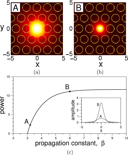
Figure 1: (a,b) Examples of stationary solutions for scalar PCF spatial solitons for $\beta=3.2$ and $\beta=6$, and (c) power dependence of the soliton family. Points A and B in the power diagram (c) correspond to the examples (a,b), respectively. Inset: the corresponding one-dimensional profiles at $y=0$ for both examples.

Figure 2: Results of numerical simulations of the soliton dynamics in the scalar case. The initial stationary solution is perturbed by two amplitude scalings (indicated in the graphs): one is higher and the other one is lower than the unity. Shown is the maximum soliton intensity vs. the propagation distance.

Figures 1(a,b) show two examples of stationary, spatially localized solutions of the nonlinear model (2) at $v=0$, which describe scalar spatial optical solitons as nonlinear modes of PCF. The whole family of such one-parameter solutions can be characterized by the power $P=\int u^{2}dxdy$, that is plotted in Fig. 1(c), where the points A and B correspond to the examples (a,b), respectively. The material parameters for the PCF are taken as $n_{a}=1$, $n_{s}=4$ and $r=0.75$.

First, we notice that these stationary solutions for scalar spatial solitons in PCF have been found earlier by Ferrando et al. Ferrando2003 , who also mentioned, without a proof, that such nonlinear modes are stabilized by the lattices of PCF holes. Indeed, it is well known that in the nonlinear focusing Kerr media without a nonlinearity saturation, the self-trapped optical beams are always unstable book . This instability can manifest itself as the beam spreading, when the input power is lower than that of the soliton, or the beam collapse, when the power is larger than the soliton power. As has been mentioned earlier by Ferrando et al. Ferrando2003 , such a soliton instability can be suppressed by the presence of the lattice of holes, because the external potential stops the beam spreading, as it happens in a conventional optical fiber, leading to the existence of a family of stable stationary beams.

In order to demonstrate this feature, we follow the standard analysis of the soliton stability book and plot in Fig. 1(c) the soliton power as a function of the soliton propagation constant. A positive slope of this dependence indicates the soliton stability, as will be demonstrated below. In Fig. 2 we present some related numerical simulations of the dynamics of a perturbed scalar soliton. Some of the stationary states are scaled by factors slightly higher and lower than the unity respectively, so as to induce an initial perturbation, and then propagated using a standard beam-propagation-method algorithm. The result is that the soliton behaves stably if its power remains below the maximal limiting power on Fig. 1(c).

When the scaling factor is taken higher than unity, a stable propagation is observed for the solitons of low enough power, as seen in Fig. 2(a). Nevertheless, for higher values of the power the soliton may collapse if the scaling factor is too large [Fig. 2(b)], but it remains stable for a smaller scaling, see Fig. 2(c). Further increase in the initial power results in collapse of the beam for any scaling factor (Fig. 2(d)).

When the scaling factor is taken smaller than unity, the lattice of holes stops the soliton spreading in all cases, so that the soliton propagates stable, as is illustrated in all cases presented in Fig. 2.

IV.2 Vector solitons

Vector solitons in the coupled problem (2) depend on both propagation constants $(\beta,\gamma$) as well as the material parameters $(\delta,\mu)$. Some examples of the vector solitons in PCF are presented in Fig. 3, corresponding to the points A and B marked on the existence domain shown in Fig. 4. This domain, whose symmetry respect both parameters $\beta$ and $\gamma$ is evident from the symmetry of both the equations of the model (2), is plotted in the plane $(\beta,\gamma)$. The existence domain is limited by two lines at whose points (bifurcation points) the vector solitons originate from the scalar solitons; such curves can be regarded as bifurcation curves. When $\mu<1$, close to the lower bifurcation curve, the second component decreases becoming a linear guided mode of the soliton mode in the first (self-guided) component; the opposite case occurs close to the upper bifurcation curve where the role of the components is reversed. When $\mu>1$, we have the opposed situation with respect to the lower and upper bifurcation curves. The presence of an effective waveguide associated with one missing hole in the lattice is the reason that the propagation constants take a value different from zero, when the power vanishes; this threshold value corresponds to the eigenvalue of the linear mode guided by this effective waveguide in the lattice of air-holes.

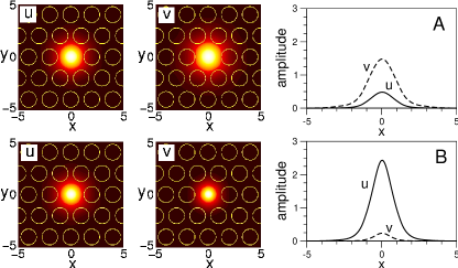
Figure 3: Examples of the two-component stationary solutions of the model (2) for vector solitons in PCFs. Two cases correspond to the points A ($\beta=5,\gamma=4$) and B ($\beta=5,\gamma=8$) in the existence domain shown in Fig. 4 for $\mu=2$. In each column both components are shown in the plane $(x,y)$, together with a one-dimensional $x$-cutoff profile to compare the field amplitudes.

Similar to the scalar case, the presence of a periodic lattice of holes suggests that the vector solitons may become stable in this system. In this case, the vectorial nature of the system plays an important role to determine the portion of the domain where the solutions are stable. As follows from the next section, by applying the generalized matrix stability criterion, it is possible to determine the boundary between the stable and unstable regions. According to that, this boundary is the set of points that fulfill the marginal stability condition $\det(D)=0$, where $D_{ij}=\partial P_{i}/\partial\beta_{j}$ while $(P_{1},P_{2})$ and $(\beta_{1},\beta_{2})$ are respectively powers and propagation constants for the components $(u,v)$. In Fig. 4 this boundary, as well as both regions of stability and instability are represented. A number of numerical simulations were carried out to test the stability of the solutions in each region. A standard beam propagation algorithm was used and the stationary solutions of the system were rescaled by a constant slightly higher that one, so that the peak amplitude of the fields initially raises over the peak amplitude of the exact stationary solution. For fields in the stability region, in spite of the initial growth of amplitude, it becomes stable after certain propagation distance.

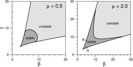
Figure 4: Existence domain for the vector solitons in PCF in the plane ($\beta$, $\gamma$), shown at two values of the coupling parameter $\mu$. Labeled points correspond to two particular examples shown in Fig. 3.

V Soliton stability

Stability of scalar and vector solitons in the coupled NLS equation can be studied with the matrix stability criterion PRE_00 ; Pel05 . Applications of the matrix criterion depend on the exact count on the number of eigenvalues of the matrix Schrödinger operators and require careful numerical computations of a spectral (linearization) problem. Alternatively, a count of the eigenvalues can be developed in a local neighborhood of the bifurcation curves, such as the ones shown on Fig. 4. These computations can be developed analytically, with the perturbation series expansions PY00 ; PY03 ; PY05 .

V.1 Scalar solitons

For simplicity and without loss of generality, we set $n_{a}=0$ in our analytical computations. First, we study the stability of scalar solitons, when $u=\phi(x,y)$ and $v=0$, where $\phi(x,y)$ is a solution of the nonlinear eigenvalue problem:

$$\Delta\phi-\beta\phi+V(x,y)\left(\delta+\phi^{2}\right)\phi=0,$$ (6)

We assume that there exists a ground state (positive definite) solution of the linear problem

$$\Delta\phi_{0}-\beta_{0}\phi_{0}+\delta V(x,y)\phi_{0}=0.$$

with the propagation constant $\beta_{0}$. Applying the local bifurcation analysis for the nonlinear ground state, we look for the solutions in the asymptotic form, $\phi=\epsilon[\phi_{0}+\epsilon^{2}\phi_{2}+{\rm O}(\epsilon^{4})]$ and $\beta=\beta_{0}+\epsilon^{2}\beta_{2}+{\rm O}(\epsilon^{4})$, and obtain the result

$$\beta_{2}=\frac{(\phi_{0}^{2},V(x,y)\phi_{0}^{2})}{(\phi_{0},\phi_{0})}>0,$$ (7)

where the inequality follows from the fact that $V(x,y)$ is non-negative. Therefore, the soliton power (squared $L^{2}$ norm) $p(\beta)=\|\phi\|_{L^{2}}^{2}=(\phi,\phi)$ is an increasing function of the propagation constant $\beta$ near the bifurcation point $\beta=\beta_{0}$:

$$\frac{dp}{d\beta}=\frac{(\phi_{0},\phi_{0})}{\beta_{2}}+{\rm O}(\epsilon^{2})>0.$$ (8)

Stability for the scalar solitons is determined by the linear eigenvalue problem, $L_{+}u=-\lambda w$ and $L_{-}w=\lambda u$, where the linear operators $L_{\pm}$ are defined as,

$$L_{+} = \beta-\Delta-V(x,y)\left(\delta+3\phi^{2}(x,y)\right)$$

$$L_{-} = \beta-\Delta-V(x,y)\left(\delta+\phi^{2}(x,y)\right).$$

If $\phi(x,y)>0$ for all $(x,y)\in R^{2}$, then $L_{-}$ is non-negative with the zero eigenvalue $L_{-}\phi=0$ due to the gauge invariance. We shall consider the number of negative eigenvalues of $L_{+}$ and apply the earlier results for one-dimensional solitons PRE_00 . It is clear that $L_{+}$ must have at least one negative eigenvalue, since

$$(\phi,L_{+}\phi)=-2(\phi^{2},V(x,y)\phi^{2})<0$$ (9)

When $\beta=\beta_{0}$ and $\phi=0$, the operator $L_{+}$ has a simple zero eigenvalue and no negative eigenvalues. Therefore, according to the perturbation theory, the operator $L_{+}$ has exactly one negative eigenvalue for $\beta>\beta_{0}$ near the local bifurcation threshold. The condition for applicability of the Vakhitov-Kolokolov criterion is satisfied and it suggests stability of scalar solitons at least near the bifurcation point.

Numerically, we have checked that the number of negative eigenvalues of $L_{+}$ does not change and the slope of $dP/d\beta$ is always positive, as shown in the example presented in Fig. 1(c). Therefore, the scalar optical solitons in PCF is stable everywhere for $\beta>\beta_{0}$.

V.2 Vector solitons

Next, we study stability of vector solitons, when $u=\Phi(x,y)$ and $v=\Psi(x,y)$, where $\Phi(x,y)$ and $\Psi(x,y)$ are real-valued positive solutions of the coupled nonlinear eigenvalue problem:

$$\begin{array}[]{l}{\displaystyle\beta\Phi=\Delta\Phi+V(x,y)\left(\delta+\Phi^{2}+\mu\Psi^{2}\right)\Phi,}\\[9.0pt] {\displaystyle\gamma\Psi=\Delta\Psi+V(x,y)\left(\delta+\mu\Phi^{2}+\Psi^{2}\right)\Psi,}\end{array}$$ (10)

We consider a local bifurcation of the vector soliton from the scalar one, and look for solutions in the asymptotic form, $\Phi=\Phi_{0}+\epsilon^{2}\Phi_{2}+{\rm O}(\epsilon^{4})$, $\Psi=\epsilon(\Psi_{0}+\epsilon^{2}\Psi_{2}+{\rm O}(\epsilon^{4}))$, and also expand the eigenvalue, $\gamma=\gamma_{0}+\epsilon^{2}\gamma_{2}+{\rm O}(\epsilon^{4})$, where $\beta$ is an arbitrary parameter, such that $\beta>\beta_{0}$. The function $\Phi_{0}=\phi(x,y)$ satisfies the nonlinear eigenvalue problem (6) for a scalar soliton. Function $\Psi_{0}=\psi(x,y)$ is a ground state solution of the linear eigenvalue problem:

$$L_{0}\psi=\left(\gamma_{0}-\Delta-V(x,y)\left(\delta+\mu\phi^{2}\right)\right)\psi=0,$$ (11)

where $\gamma_{0}$ is a function of parameters ($\delta,\mu$) and the propagation constant $\beta$. The problem for $\Phi_{2}(x,y)$, $L_{+}\Phi_{2}=\mu V(x,y)\phi\psi^{2}$, is always solvable, in the assumption that the operator $L_{+}$ for the scalar soliton has one negative and no zero eigenvalues for any $\beta>\beta_{0}$. Finally, from the solvability condition of the linear inhomogeneous problem,

$$L_{0}\Psi_{2}=2\mu V(x,y)\phi\psi\Phi_{2}+V(x,y)\psi^{3}-\gamma_{2}\psi,$$ (12)

we derive that

$$\gamma_{2}=\frac{2\mu(\psi^{2},V(x,y)\phi\Phi_{2})+(\psi^{2},V(x,y)\psi^{2})}{(\psi,\psi)}.$$

Numerical results show that $\gamma_{2}>0$ for $\mu<1$ (i.e. the bifurcation occurs from the lower boundary of the existence domain on the plane $(\beta,\gamma)$), $\gamma_{2}<0$ for $\mu>1$ (i.e. bifurcation occurs from the upper boundary of the existence domain), and $\gamma_{2}=0$ for $\mu=1$ (i.e. the existence domain shrinks on the diagonal $\gamma=\beta>\beta_{0}$ and $\gamma_{0}=\beta_{0}$.)

We compute the Hessian matrix of derivatives of individual powers $P=(\Phi,\Phi)$ and $Q=(\Psi,\Psi)$ with respect to parameters $\beta$ and $\gamma$. Let $p=(\phi,\phi)$ and assume that $p^{\prime}(\beta)>0$ for scalar soliton with $\beta>\beta_{0}$. Near the local bifurcation threshold at $\gamma=\gamma_{0}$, we have:

$$\frac{\partial P}{\partial\gamma}=\frac{2(\phi,\Phi_{2})}{\gamma_{2}}+{\rm O}(\epsilon^{2})=\frac{\partial Q}{\partial\beta},\qquad\frac{\partial Q}{\partial\gamma}=\frac{(\psi,\psi)}{\gamma_{2}}+{\rm O}(\epsilon^{2}),$$ (13)

such that the determinant of the Hessian matrix is

$$D(\beta,\gamma)=\frac{(\psi,\psi)p^{\prime}(\beta)}{\gamma_{2}}-\frac{4(\phi,\Phi_{2})^{2}}{\gamma_{2}^{2}}+{\rm O}(\epsilon^{2}).$$ (14)

When $\mu<1$, we have $\gamma_{2}>0$ and the determinant may change the sign. Numerical results show that $D>0$ for $\beta_{0}<\beta<\beta_{*}$ and $D<0$ for $\beta>\beta_{*}$ near the local bifurcation boundary $\gamma=\gamma_{0}$.

When $\mu>1$, we have $\gamma_{2}<0$ and the determinant is always negative near the local bifurcation boundary $\gamma=\gamma_{0}$. When $\mu=1$, we have $\beta=\gamma$ and $P=Q$, such that $D=0$.

With the standard linearization, the stability problem for vector solitons reduces to the matrix eigenvalue problem $\hat{L}_{+}{\bf u}=-\lambda{\bf w}$ and $\hat{L}_{-}{\bf w}=\lambda{\bf u}$, where ${\bf u}$ is a two-vector of real parts of the perturbation and ${\bf w}$ is a two-vector of imaginary parts of the perturbation, for a real eigenvalue $\lambda$. The matrix Schrodinger operators are

$$\hat{L}_{+}=\left(\begin{array}[]{ccc}\beta-\Delta-V(\delta+3\Phi^{2}+\mu\Psi^{2})&-2\mu V\Phi\Psi\\ -2\mu V\Phi\Psi&\gamma-\Delta-V(\delta+3\Psi^{2}+\mu\Phi^{2})\end{array}\right)$$

$$\hat{L}_{-}=\left(\begin{array}[]{ccc}\beta-\Delta-V(\delta+\Phi^{2}+\mu\Psi^{2})&0\\ 0&\gamma-\Delta-V(\delta+\Psi^{2}+\mu\Phi^{2})\end{array}\right)$$

Since $\hat{L}_{-}$ is a diagonal composition of two scalar Schrödinger operators, each has a simple zero eigenvalue with the ground state $\Phi$ and $\Psi$, therefore, the operator $\hat{L}_{-}$ is non-negative. Therefore, stability of fundamental vector solitons is determined by the number of negative eigenvalues of the matrix operator $\hat{L}_{+}$, similar to Ref. PRE_00 .

We compute the number of negative eigenvalues of the operator $\hat{L}_{+}$ near the local bifurcation point. When $\gamma=\gamma_{0}$ and $\Psi=0$, we have

$$\hat{L}_{+}=\left(\begin{array}[]{ccc}L_{+}&0\\ 0&L_{0}\end{array}\right)$$ (15)

such that the operator $L_{+}$ has exactly one negative eigenvalue (by the assumption that the scalar soliton is stable for $\beta>\beta_{0}$) and the operator $L_{0}$ has a simple zero eigenvalue with the eigenfunction $\psi$. We study bifurcation of the simple zero eigenvalue of $L_{0}$ for $\gamma\neq\gamma_{0}$. Using the same small parameter $\epsilon$ as in the local bifurcation analysis, we are looking for solution of the eigenvalue problem $\hat{L}_{+}{\bf u}=\lambda{\bf u}$ by the regular perturbation theory: $u_{1}=\epsilon U_{1}+{\rm O}(\epsilon^{3})$, $u_{2}=\psi+\epsilon^{2}U_{2}+{\rm O}(\epsilon^{4})$, and $\lambda=\epsilon^{2}\lambda_{2}+{\rm O}(\epsilon^{4})$.

By algorithmic computations of the regular perturbation theory, we have the linear inhomogeneous problem for the first-order correction, $L_{+}U_{1}=2\mu V(x,y)\phi\psi^{2}$, which is solvable with the solution $U_{1}=2\Phi_{2}$. Furthermore, we have the linear inhomogeneous problem for $U_{2}$,

$$L_{0}U_{2}=(\lambda_{2}-\gamma_{2})\psi+2\mu V(x,y)\phi\psi\Phi_{2}+3V(x,y)\psi^{3}+2\mu V(x,y)\phi\psi U_{1},$$

with the solvability condition:

$$\lambda_{2}=\gamma_{2}-\frac{6\mu(\psi^{2},V(x,y)\phi\Phi_{2})+3(\psi^{2},V(x,y)\psi^{2})}{(\psi,\psi)}=-2\gamma_{2}.$$

When $\mu<1$, we have $\gamma_{2}>0$, such that the zero eigenvalue of $L_{0}$ becomes a negative eigenvalue of $\hat{L}_{+}$. As a result, we have two negative eigenvalues of $\hat{L}_{+}$ near the local bifurcation boundary. Since $p^{\prime}(\beta)>0$, we have two positive eigenvalues of the Hessian matrix when $D>0$ and one positive eigenvalue when $D<0$. In the former case, the vector soliton is stable, while it is unstable in the latter case. Therefore, the boundary of $D=0$ separate the domains of stability and instability of vector solitons on the plane $(\beta,\gamma)$ in the assumption that the number of negative eigenvalues of $\hat{L}_{+}$ remains unchanged in the entire existence domain.

When $\mu>1$, we have $\gamma_{2}<0$, such that the zero eigenvalue of $L_{0}$ becomes a positive eigenvalue of $\hat{L}_{+}$. As a result, we have only one negative eigenvalue of $\hat{L}_{+}$ near the local bifurcation boundary. In the same region, we have exactly one positive eigenvalue of the Hessian matrix, since $D<0$. Therefore, the vector soliton is stable near the local bifurcation boundary. Numerics show that there exists a curve $D=0$ in the existence domain (see Fig. 4(b)), where the positive eigenvalue of the Hessian matrix crosses zero and becomes negative eigenvalue. These curve approaches the bifurcation curves asymptotically for large $(\beta,\gamma)$, since $D<0$ on the bifurcation curves. In the assumption that the number of negative eigenvalues of $\hat{L}_{+}$ remains unchanged in the entire existence domain, the curve $D=0$ separates the stability and instability domains.

When $\mu=1$, we have $\gamma=\beta$ and the zero eigenvalue of $L_{0}$ is preserved as the zero eigenvalue of $\hat{L}_{+}$ in the entire existence domain $\beta=\gamma>\beta_{0}$. This additional eigenvalue is related to an arbitrary polarization of the vector soliton in the case $\mu=1$: $\Phi=\cos\theta\;\phi$ and $\Psi=\sin\theta\;\phi$, where $\phi$ solves the scalar problem (6). The operator $\hat{L}_{+}$ always has a single negative eigenvalue (since we have verified numerically that $L_{+}$ has a single negative eigenvalue for $\beta>\beta_{0}$). Therefore, the vector soliton must be linearly stable in the case $\mu=1$ for any $\beta>\beta_{0}$ (excluding the limit $\beta\to\infty$).

VI Conclusions

We have demonstrated that stable two-dimensional vector solitons can be supported by a nonlinear PCF structure with the Kerr nonlinearity. They constitute a class of two-component spatially localized modes that bifurcate from their one-component scalar counterparts and are described by two independent parameters. Both scalar and vector solitons provide a generalization of the guided mode trapped in the PCF core to the nonlinear case, being confined by both linear and self-induced nonlinear refractive indices. The periodic PCF environment provides also an effective stabilization mechanism for these localized modes, in a sharp contrast with an entirely homogeneous nonlinear Kerr medium where both scalar and vector spatial solitons are unstable and may undergo the collapse instability. We have applied the analytical matrix criterion for stability of these PCF vector solitons, and have verified that this criterion is confirmed by the direct simulations of the soliton dynamics.

VII Acknowledgments

This work has been supported in part by the Australian Research Council. JRS acknowledges a visiting fellowship granted by the Dirección Xeral de Investigación e Desenvolvemento of Xunta de Galicia (Spain). Both JRS and DEP thank Nonlinear Physics Center at the Australian National University for a warm hospitality during their stay in Canberra.

References

- (1) P. Russell, Science 299, 358 (2003)
- (2) J.C. Knight, Nature 424, 847 (2003).
- (3) Yu.S. Kivshar and G.P. Agrawal, Optical Solitons: From Fibers to Photonic Crystals (Academic, San Diego, 2003).
- (4) Y. V. Kartashov, A. S. Zelenina, V. A. Vysloukh, and L. Torner, Phys. Rev. E 70, 066623 (2004).
- (5) Z. Chen, A. Bezryadina, I. Makasyuk, and J. Yang, Opt. Lett. 29, 1656 (2004).
- (6) S.F. Mingaleev, and Yu.S. Kivshar, Phys. Rev. Lett. 86, 5474 (2001).
- (7) A. Ferrando, M. Zacarés, P. Fernandez de Córdoba, D. Binosi, and J.A. Monsoriu, Opt. Exp. 11, 452 (2003).
- (8) A. Ferrando, M. Zacarés, P. Fernandez de Córdoba, D. Binosi, and J.A. Monsoriu, Opt. Exp. 12, 817 (2004).
- (9) J.N. Malmberg, A.H. Carlsson, D. Anderson, M. Lisak, E.A. Ostrovskaya, and Yu.S. Kivshar, Opt. Lett. 25, 643 (2000).
- (10) J. E. Dennis and R. B. Schnabel, Numerical Methods for Unconstrained Optimization and Nonlinear Equations (Englewood Cliffs, NJ: Prentice-Hall, 1983)
- (11) W. H. Press, S. A. Teukolsky, W. T. Vetterling, B. P. Flannery, Numerical recipes in C (Cambridge University Press, Cambridge, 2nd ed. 1992).
- (12) C. C. Paige and M. A. Saunders, SIAM J. Numer. Anal. 12, 617 (1975).
- (13) D.E. Pelinovsky and Yu.S. Kivshar, Phys. Rev. E 62, 8668 (2000).
- (14) D.E. Pelinovsky, Proc. Roy. Soc. Lond. A 461, 783 (2005)
- (15) D.E. Pelinovsky and J. Yang, Stud. Appl. Math. 105, 245 (2000).
- (16) J. Yang and D.E. Pelinovsky, Phys. Rev. E 67, 016608 (2003).
- (17) D.E. Pelinovsky and J. Yang, Stud. Appl. Math., in print (2005).