Analytical and Numerical Investigation of the Phase–Locked Loop with Time Delay

Abstract

We derive the normal form for the delay–induced Hopf bifurcation in the first–order phase–locked loop with time delay by the multiple scaling method. The resulting periodic orbit is confirmed by numerical simulations. Further detailed numerical investigations demonstrate exemplarily that this system reveals a rich dynamical behavior. With phase portraits, Fourier analysis and Lyapunov spectra it is possible to analyze the scaling properties of the control parameter in the period–doubling scenario, both qualitatively and quantitatively. Within the numerical accuracy there is evidence that the scaling constant of the time–delayed phase–locked loop coincides with the Feigenbaum constant $\delta\approx 4.669$ in one–dimensional discrete systems.

I Introduction

Many nonlinear dynamical systems in various scientific disciplines are influenced by the finite propagation time of signals in feedback loops. A typical physical system is provided by a laser where the output light is reflected and fed back to the cavity laser1 ; laser2 . But time delays also occur in biology due to physiological control mechanisms neuro1 ; neuro2 or in economy where the finite velocity of information processing has to be taken into account econo1 ; econo2 . Furthermore, realistic models in population dynamics or in ecology include the duration for the replacement of resources popu1 ; popu2 .

All these different systems have in common that the inherent time delay may induce dynamical instabilities. Numerous experimental and theoretical studies have demonstrated this for the emergence of oscillatory behavior, quasi-periodicity, chaos or intermittency. But time–delayed feedbacks can also have the opposite effect. They have even been devised to stabilize previously unstable stationary states or limit cycles stab1 ; stab2 ; stab3 . In particular this method allows to control or to prevent undesirable chaotic behavior in a time–continuous way. In comparison with the time–discrete method of Ott, Grebogi, and Yorke ogi it can be easier implemented as it relies on less information of the dynamical system.

The choice of a paradigmatic model system for analyzing the fundamental properties of delay–induced instabilities is determined by several practical conditions. On the one hand it should be guaranteed that all observable instabilities are purely a result of time delays. On the other hand the dynamics should be governed by a simple model equation and allow for a quantitative comparison between theory and experiment. These conditions are fulfilled, for instance, by the Mackey–Glass model neuro1 which describes quite successfully the anomalies in the regeneration of white blood cells. However the underlying nonlinear scalar delay differential equation necessitates three effective control parameters to account for the experimental data.

In this article we report about analytical and numerical investigations of the rich dynamical behavior of another model system which was proposed some time ago by Wischert et al. in Ref. Wolfgang . It represents the first–order phase–locked loop (PLL) with time delay which synchronizes the phases of two oscillators. In comparison with the Mackey–Glass model, this system has the advantage that it involves only a single effective control parameter instead of three. Additionally, it can be realized electronically under well–defined conditions. Furthermore, an extension of the PLL with time delay is capable of describing sensibly physiological control experiments Peter .

The experimental set–up for the electronic system of a first–order phase–locked loop (PLL) is shown in Fig. 3 of Ref. Wolfgang . In many applications the PLL serves for synchronizing the phases of a reference oscillator and a voltage–controlled oscillator (VCO). Thereby the frequency of the output signal of the VCO depends linearly on the input signal. The output signals of both oscillators are multiplied by the aid of a mixer. The induced high–frequency components are then eliminated by a low–pass filter. The resulting signal is fed back to the input of the VCO. A delay line between the VCO and the mixer, implemented analogously or numerically, induces the time delay $\tau\geq 0$.

The dynamical variable of interest is the phase difference $q(t)$ between both incoming signals of the mixer (compare with Fig. 3 of Ref. Wolfgang ). Under quite simple assumptions it becomes possible to derive a nonlinear scalar delay differential equation for this phase difference Wolfgang :

$$\frac{d}{dt}q(t)=-K\,\sin[q(t-\tau)]\,.$$ (1)

The parameter $K\geq 0$ denotes the so-called open loop gain of the PLL. Performing an appropriate scaling of the time converts the PLL equation (1) to its standard form

$$\frac{d}{dt}q(t)=-R\,\sin[q(t-1)]\,,$$ (2)

where the two parameters $\tau,K$ are reduced to one effective control parameter

$$R=K\tau\,.$$ (3)

Thus varying the delay time $\tau$ corresponds to changing the control parameter $R$. In this paper we analyze both analytically and numerically the rich structure of delay–induced instabilities of the PLL equation (2). In Section II we derive the normal form of the Hopf bifurcation by applying the multiple scaling method. The emerging periodic orbit is confirmed in Section III by numerical simulations. In Section IV we study in detail the period–doubling scenario beyond the Hopf bifurcation with phase portraits, Fourier analysis and Lyapunov spectra.

II Multiple Scaling Method

Applying the synergetic system analysis it was shown in Ref. Wolfgang that a Hopf bifurcation occurs in the PLL equation (2) at the critical value $R_{c}=\pi/2$. In the following we rederive the normal form of this Hopf bifurcation by using the multiple scaling method Michael1 . It represents a systematic technical procedure to deduce the normal form by using an ansatz how the respective quantities depend on the smallness parameter

$$\varepsilon=\frac{R-R_{c}}{R_{c}}\quad\Longleftrightarrow\quad R=R_{c}(1+\varepsilon)\,.$$ (4)

Although the multiple scaling method has been originally developed for ordinary or partial differential equations ms1 ; ms2 ; ms3 ; Bender ; Manneville , it can be also applied to delay differential equations (see, for instance, the treatment in Ref. elena ).

We start with discussing some properties of the Hopf bifurcation. At first, we mention that the amplitude of the emerging periodic solution has a characteristic $\varepsilon^{1/2}$–dependence from the smallness parameter $\varepsilon$, as can be deduced from the linear stability analysis already presented in Ref. Wolfgang . Furthermore, the trajectory approaches the limit cycle slowly near the instability due to the phenomenon of critical slowing down. Thus the oscillatory solution $q(t)$ of the PLL equation (2) is based on two different time scales. The fast time scale is provided by the period $T=2\pi/\Omega$ of the oscillatory solution, whereas the slow one characterizes the amplitude dynamics in the transient regime. Both time scales are separated by a factor of the smallness parameter $\varepsilon$, as follows again from the linear stability analysis Wolfgang . These considerations lead to the following ansatz for the oscillatory solution after the Hopf bifurcation:

$$q(t) = q_{\rm stat}+\varepsilon^{1/2}\left[q_{0}^{+}(t^{\prime})e^{i\Omega t}+q_{0}^{-}(t^{\prime})e^{-i\Omega t}\right]+\varepsilon\left[q_{2}^{+}(t^{\prime})e^{2i\Omega t}+q_{1}(t^{\prime})+q_{2}^{-}(t^{\prime})e^{-2i\Omega t}\right]$$ (5)

$$+\varepsilon^{3/2}\left[q_{4}^{+}(t^{\prime})e^{3i\Omega t}+q_{3}^{+}(t^{\prime})e^{i\Omega t}+q_{3}^{-}(t^{\prime})e^{-i\Omega t}+q_{4}^{-}(t^{\prime})e^{-3i\Omega t}\right]+{\cal O}\left(\varepsilon^{2}\right)\,.$$

Here the first time scale $t$ and the second time scale $t^{\prime}$ are related via

$$t^{\prime}=\varepsilon\,t\,,$$ (6)

where the smallness parameter $\varepsilon$ denotes the deviation from the bifurcation point according to (4), and the respective amplitudes have the properties

$$q_{k}^{\pm}(t^{\prime})={q_{k}^{\mp}{}(t^{\prime})}^{*}\,,\quad k=0,2,3,4\,;\quad\quad q_{1}(t^{\prime})=q_{1}(t^{\prime})^{*}\,.$$ (7)

Now we insert our ansatz (5) in the PLL equation (2). By doing so, we have to take into account that the slowly varying amplitudes $q_{i}^{\pm}(t^{\prime})$ have the time derivative

$$\frac{d}{dt}q_{i}^{\pm}(t^{\prime})=\varepsilon\,\frac{d}{dt^{\prime}}q_{i}^{\pm}(t^{\prime})$$ (8)

and that their time delay results in the expansion

$$q_{i}^{\pm}(t^{\prime}-\varepsilon)=q_{i}^{\pm}(t^{\prime})-\varepsilon\,\frac{d}{dt^{\prime}}q_{i}^{\pm}(t^{\prime})+{\cal O}(\varepsilon^{2})\,.$$ (9)

The strategy is then to compare all those terms with each other which have the same power in the smallness parameter $\varepsilon$. Thereby we have to guarantee that in each order the respective Fourier coefficients compensate each other:

• In the lowest order $\varepsilon^{0}$ we have only the frequency $0$ which leads to the equality

  $$R_{c}\,\sin(q_{\rm stat})=0\,.$$ (10)

  This fixes the stationary state to be

  $$q_{\rm stat}=l\,\pi\,,\quad l=0,\pm 1,\pm 2,\ldots\,.$$ (11)

  In the following we restrict ourselves to consider the reference state $q_{\rm stat}^{\rm I}=0$ as the other one $q_{\rm stat}^{\rm II}=\pi$ turns out to be unstable for all values of the control parameter $R$.

• The order $\varepsilon^{1/2}$ contains only the frequency $\pm\Omega$ with the condition

  $$\pm i\Omega\,q_{0}^{\pm}(t^{\prime})=-R_{c}e^{\mp i\Omega}\,q_{0}^{\pm}(t^{\prime})\,.$$ (12)

  As the amplitudes $q_{0}^{\pm}(t^{\prime})$ should not vanish, we conclude

  $$-R_{c}e^{\mp i\Omega}\mp i\Omega=0\,.$$ (13)

  This condition coincides with the transcendental characteristic equation (98) of the linear stability analysis of Ref. Wolfgang if the eigenvalues $\lambda$ at the instability are identified according to $\lambda=i\Omega$. The real part of Eq. (13)

  $$\cos\Omega=0$$ (14)

  leads to the frequency

  $$\Omega=\frac{\pi}{2}\,,$$ (15)

  whereas the imaginary part results in the critical value of the control parameter:

  $$R_{c}=\frac{\pi}{2}\,.$$ (16)

• The order $\varepsilon$ involves two frequency components. The Fourier coefficients of the frequency $0$ immediately lead to

  $$q_{1}(t^{\prime})=0\,,$$ (17)

  and for the frequency $\pm 2\Omega$ we obtain

  $$\pm 2i\Omega q_{2}^{\pm}(t^{\prime})=-R_{c}e^{\mp 2i\Omega}q_{2}^{\pm}(t^{\prime})\,,$$ (18)

  which reduces due to the characteristic equation (13) to

  $$q_{2}^{\pm}(t^{\prime})=0\,.$$ (19)

• Also the order $\varepsilon^{3/2}$ consists of two frequency components. For the frequency $\pm\Omega$ we read off

  $$\left(1-R_{c}e^{\mp i\Omega}\right)\frac{d}{dt^{\prime}}q_{0}^{\pm}(t^{\prime})=\left(-R_{c}e^{\mp i\Omega}\mp i\Omega\right)q_{3}^{\pm}(t^{\prime})-\frac{1}{2}R_{c}e^{\mp i\Omega}\left[2q_{0}^{\pm}(t^{\prime})-{q_{0}^{\pm}(t^{\prime})}^{2}q_{0}^{\mp}(t^{\prime})\right]\,.$$ (20)

  The factor in front of $q_{3}^{\pm}(t^{\prime})$ vanishes because of the characteristic equation (13). Thus the functions $q_{3}^{\pm}(t^{\prime})$ are not determined in this order, they only follow from the next order $\varepsilon^{2}$ and the frequency $\pm\Omega$. Taking into account the characteristic equation (13), we yield from (20) the normal form of the order parameter equation:

  $$\frac{d}{dt^{\prime}}q_{0}^{\pm}(t^{\prime})=A^{\pm}q_{0}^{\pm}(t^{\prime})+B^{\pm}{q_{0}^{\pm}(t^{\prime})}^{2}q_{0}^{\mp}(t^{\prime})\,.$$ (21)

  There the parameters $A^{\pm}$ and $B^{\pm}$ are defined by

  $$A^{\pm}=\frac{iR_{c}}{1+iR_{c}}\,,\quad B^{\pm}=-\frac{A^{\pm}}{2}\,.$$ (22)

  Note that the normal form (21) of the multiple scaling method and the normal form of the synergetic system analysis in Ref. Wolfgang do not coincide, however, they can be mapped into each other using an appropriate coordinate transformation Michael1 . Correspondingly, we obtain for the frequency $\pm 3\Omega$

  $$\pm 3i\Omega q_{4}^{\pm}(t^{\prime})=\frac{1}{6}R_{c}e^{\mp 3i\Omega}\left[{q_{0}^{\pm}(t^{\prime})}^{3}-6q_{4}^{\pm}(t^{\prime})\right]\,,$$ (23)

  which reduces due to (13), (15) and (16) to

  $$q_{4}^{\pm}(t^{\prime})=\frac{1}{24}{q_{0}^{\pm}(t^{\prime})}^{3}\,.$$ (24)

  As the functions $q_{3}^{\pm}(t^{\prime})$ and $q_{4}^{\pm}(t^{\prime})$ are of the order $\varepsilon^{3/2}$ according to the ansatz (5), they are irrelevant for the order $\varepsilon$ in which we are interested.

It remains to solve the order parameter equation (21), (22) by using polar coordinates

$$q_{0}^{\pm}(t^{\prime})=R(t^{\prime})\,e^{\pm i\varphi(t^{\prime})}\,.$$ (25)

The resulting stationary solution turns out to be

$$R(t^{\prime})=\sqrt{2}+{\cal O}(\varepsilon^{2})$$ (26)

together with the phase

$$\varphi(t)=\Omega(\varepsilon)t+\varphi_{0}\,.$$ (27)

Here the frequency turns out to be

$$\Omega(\varepsilon)=R_{c}+{\cal O}(\varepsilon^{2})\,.$$ (28)

Thus we conclude from (15), (17), (19), (26), (27), and (28) that the oscillatory solution after the Hopf bifurcation reads

$$q(t)=c_{0}(\varepsilon)+c_{1}(\varepsilon)\cos\left[\varphi(t)+\psi_{1}\right]+c_{2}(\varepsilon)\cos\left[2\varphi(t)+\psi_{2}\right]+{\cal O}\left(\varepsilon^{3/2}\right)\,,$$ (29)

where the respective coefficients read

$$c_{0}(\varepsilon)=0+{\cal O}\left(\varepsilon^{2}\right)\,,\quad c_{1}(\varepsilon)=\sqrt{8\varepsilon}+{\cal O}\left(\varepsilon^{3/2}\right)\,,\quad c_{2}(\varepsilon)=0+{\cal O}\left(\varepsilon^{2}\right)\,.$$ (30)

It coincides with the result of the synergetic system analysis in Ref. Wolfgang up to the order $\varepsilon$. Although we restrict ourselves to this order, the systematics of the multiple scaling method is obvious, thus an extension of the ansatz (5) to higher orders is straight–forward, but the calculation would become quite cumbersome.

III Numerical Verification

In order to numerically verify our analytical result, we integrated the underlying PLL equation (2). By doing so, we varied the control parameter $R$ in the vicinity of the instability $R_{c}=\pi/2$ in such a way that the smallness parameter $\varepsilon=(R-R_{c})/R_{c}$ took 200 equidistant values between $10^{-5}$ and $10^{-1}$. We used a Runge–Kutta–Verner method of the IMSL library as an integration routine and performed a linear interpolation between the respective values. In particular in the immediate vicinity of the instability the phenomenon of critical slowing down led to a transient behavior. To exclude this, we iterated the discretized delay differential equation for each value of the control parameter at least $10^{6}$ times. Afterwards we calculated the power spectrum with a complex FFT so that the basic frequency $\Omega$ of the oscillatory solution could be determined with high resolution. Then we performed a real FFT with the period $T=2\pi/\Omega$ of the simulated periodic signal $q(t)=q(t+T)$:

$$q(t)=\frac{a_{0}}{2}+\sum_{k=1}^{\infty}\left[a_{k}\cos\left(k\Omega t\right)+b_{k}\sin\left(k\Omega t\right)\right]\,.$$ (31)

investigated quantity	analytical expression		analytical value		numerical value
$A$	$A(0)$	$\left.\frac{dA}{d\varepsilon}\right|_{\varepsilon=0}$	$A(0)$	$\left.\frac{dA}{d\varepsilon}\right|_{\varepsilon=0}$	$A(0)$	$\left.\frac{dA}{d\varepsilon}\right|_{\varepsilon=0}$
$\Omega$	${\displaystyle\frac{\pi}{2}}$	$0$	$1.5708$	$0.0$	$1.5708$	$10^{-8}$
$c_{0}$	$0$	$0$	$0.0$	$0.0$	$-3\cdot 10^{-4}$	$-2\cdot 10^{-3}$
$\ln c_{1}$	$\frac{1}{2}\ln 8$	${\displaystyle\frac{1}{2}}$	$1.0397$	$0.5$	$1.0356$	$0.4999$
$c_{2}$	$0$	$0$	$0.0$	$0.0$	$2\cdot 10^{-4}$	$6\cdot 10^{-2}$

Table 1: Comparing the analytical and the numerical values for the frequency $\Omega(\varepsilon)$ and the Fourier coefficients $c_{0}(\varepsilon)$, $c_{1}(\varepsilon)$, $c_{2}(\varepsilon)$ of the oscillatory solution of the PLL equation after the Hopf bifurcation.

The Fourier coefficients follow from integrations with respect to one period $T=2\pi/\Omega$:

$$a_{k}=\frac{2}{T}\int\limits_{0}^{T}dt\,f(t)\,\cos\left(k\Omega t\right)\,,\quad k=0,1,\ldots,\infty\,;\quad b_{k}=\frac{2}{T}\int\limits_{0}^{T}dt\,f(t)\,\sin\left(k\Omega t\right)\,,\quad k=1,\ldots,\infty\,.$$ (32)

From (31) follows then the spectral representation

$$q(t)=c_{0}+\sum_{k=1}^{\infty}c_{k}\cos\left(k\Omega t+\phi_{k}\right)$$ (33)

with the quantities

$$c_{0}=\frac{a_{0}}{2}\,,\quad c_{k}=\sqrt{a_{k}^{2}+b_{k}^{2}}\,,\quad\phi_{k}=-\mbox{arctan}\,\frac{b_{k}}{a_{k}}\,,\quad k=1,\ldots,\infty\,.$$ (34)

Thus our analytical result (27), (29) can be interpreted as the first terms within a spectral representation (33), where the frequency $\Omega=2\pi/T$ and the Fourier coefficients $c_{0}$, $c_{1}$, $c_{2}$ are given by (28) and (30). Analyzing the Hopf bifurcation with a FFT, we numerically determinded $\Omega$, $c_{0}$, $c_{1}$, $c_{2}$ as a function of the smallness parameter $\varepsilon$. Comparing the respective numerical and analytical results, we observe some deviations for small and for large values of the smallness parameters $\varepsilon$. The former are due to the phenomenon of critical slowing down, i.e. the system stays longer in the transient state when the instability is approached, and the latter arise from the neglected higher order corrections in the analytical approach. Therefore we restricted our numerical analysis to the intermediate interval $[10^{-5},10^{-1}]$ of the smallness parameter $\varepsilon$.

In Tab. 1 we see that the analytical and numerical determined quantities agree quantitatively very well. Thus our weakly non-linear analysis for the delay–induced Hopf bifurcation in the PLL equation is numerically verified up to $\varepsilon\approx 10^{-1}$. However, this successfully tests only the order parameter concept for delay systems, as the lowest nonlinear term in the scalar delay differential equation of the PLL (2) is a cubic one. Therefore we analyzed the Wright equation Wright with a quadratic nonlinearity in a separate publication Michael2 , where we could successfully test not only the order parameter concept but also the slaving principle, i.e. the influence of the center manifold on the order parameter equations. Thus we demonstrated with the Wright equation the validity of the circular causality chain of synergetics for the Hopf bifurcation of a delay differential equation.

IV Further Numerical Results

In the following we summarize various simulations which have been performed for the delay differential equation (2) of a PLL with some initial function $q(t)$ for $-1\leq t\leq 0$ Michael1 ; Michael3 . In order to check the quality of the numerical results, standard integration routines of the Runge–Kutta type have been applied with different discretizations by adequately taking into account the delay effects.

Firstly, it turns out that the trajectory $q(t)$ is restricted for all times to the interval $[-\pi,+\pi]$ if the effective control parameter $R$ is increased from 0 to about 4.9. If the transient behavior has decayed, the resulting asymptotic dynamics could be classified as follows. For $0\leq R\leq\pi/2$ there exist two stationary states, a stable one $q_{1}=0$ and an unstable one $q_{2}=\pi$. At $R=\pi/2$ a super–stable Hopf bifurcation occurs where the previously stable stationary state $q_{\rm stat}^{\rm I}=0$ becomes unstable and a new stable limit cycle emerges Wolfgang . In the range $\pi/2\leq R\lessapprox 3.77$ this oscillatory solution shows a conspicuous point symmetry with respect to the origin of the phase portrait in Fig. 1a. This symmetry is broken at $R\approx 3.77$ as the limit cycle splits into two coexisting limit cycles Chrisi . They are depicted in Fig. 1b as the asymptotic dynamics of the initial functions $q(t)=\pm 1$ for $-1\leq t\leq 0$, respectively. Both coexisting limit cycles are symmetric to each other concerning the point symmetry with respect to the origin and remain stable up to $R\approx 4.9$. Note that the instability at $R\approx 3.77$ was not detected during the initial investigations in Ref. Wolfgang as there only Fourier spectra were analyzed.

Increasing the effective control parameter leads to a further bifurcation at $R\approx 4.105$. Fig. 1c illustrates that a new limit cycle emerges with the initial function $q(t)=2$ for $-1\leq t\leq 0$ which coexists for $4.105\lessapprox R\lessapprox 4.11$ with the two other oscillating solutions. Also this new limit cycle exhibits a point symmetry with respect to the origin of the phase portrait. At $R\approx 4.11$ this limit cycle splits into two new oscillating solutions with the initial functions $q(t)=\pm 2$ for $-1\leq t\leq 0$, so that the point symmetry is again destroyed (compare Fig. 1d). It turns out that both of them pass through a separate period–doubling scenario for $4.11\lessapprox R\lessapprox 4.175$. This is shown qualitatively by the Power spectra (see Fig. 2) for the first three period–doublings. Each of these bifurcations leads to a subsequent sub–harmonic and to corresponding higher combination frequencies. The bifurcation diagram in Fig. 3 is an overview over this period–doubling scenario. It was obtained by Poincaré sections of the trajectories using the software package AnT 4.669 AnTpaper ; AnTWWW , whereby the Poincaré conditions were $\dot{q}(t)=0$ and $q(t)\in[1,2]$.

In order to analyze a period–doubling scenario more quantitatively, it is advantageous to determine the Lyapunov exponents of the underlying dynamics. In our case this necessitates to use the common concept of Lyapunov exponents wolf and to extend it to delay differential equations Michael1 ; farmer . Thereby we have to take into account that their numerical integration is based on a discretization procedure. As a consequence, the determination of Lyapunov exponents for time–delayed dynamical systems is reducible to the calculation of Lyapunov exponents for a high–dimensional time–discrete mapping.

Fig. 4a shows the two largest Lyapunov exponents within and above the period–doubling scenario of the PLL. The enlargement of Fig. 4b clearly reveals the self–similarity of the spikes and the characteristic scaling properties. One of both Lyapunov exponents always vanishes due to the moving reference frame. The zeros of the second Lyapunov exponent coincide with the critical values of the effective control parameters $R_{0},R_{1},R_{2},\ldots$ where a period–doubling occurs. Table 2 lists the first bifurcation points and the scaling constants

$$\delta_{n}=\frac{R_{n-1}-R_{n}}{R_{n}-R_{n+1}}$$ (35)

of the effective control parameter. Within the numerical accuracy there is evidence that the scaling constants $\delta_{n}$ converge to the Feigenbaum constant $\delta\approx 4.669$ as in the case of one–dimensional time–discrete systems grossmann ; feigenbaum . If we assume this to be true then we can estimate the end of the period–doubling scenario

$$R_{\infty}=\frac{\delta R_{n+1}-R_{n}}{\delta-1}$$ (36)

from the bifurcation points in Tab. 2. The finding $R_{\infty}\approx 4.173961$ agrees quite well with the enlarged Lyapunov spectrum in Fig. 4b.

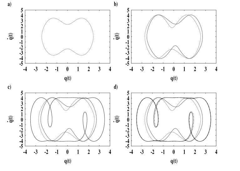
Figure 1: Phase portraits depicting several limit cycles: a) $R=3.5$, b) $R=4.1$, c) $R=4.105$ d) $R=4.11$.

Figure 2: Power spectra indicating period–doublings: a) $R=4.157$, b) $R=4.165$, c) $R=4.1725$, d) $R=4.17375$.

Figure 3: Bifurcation diagram obtained by a Poincaré section which is defined by the conditions $\dot{q}(t)=0$ and $q(t)\in[1,2]$.

Figure 4: Lyapunov spectra illustrating self–similarity. Shown are the two largest Lyapunov exponents $\lambda_{1}$ and $\lambda_{2}$.

$n$	parameter $R_{n}$	period before bifurcation	$\delta_{n}$
$0$	$4.158\pm 5\cdot 10^{-5}$	$1$	$-$
$1$	$4.1705\pm 5\cdot 10^{-5}$	$2$	$4.63\pm 2\cdot 10^{-1}$
$2$	$4.1732\pm 5\cdot 10^{-5}$	$4$	$4.49\pm 5\cdot 10^{-1}$
$3$	$4.173802\pm 5\cdot 10^{-7}$	$8$	$4.81\pm 4\cdot 10^{-1}$
$4$	$4.1739272\pm 2\cdot 10^{-7}$	$16$	$4.76\pm 10^{-1}$
$5$	$4.1739535\pm 2.5\cdot 10^{-7}$	$32$	$4.46\pm 3\cdot 10^{-1}$
$6$	$4.1739594\pm 5\cdot 10^{-8}$	$64$	$4.72\pm 4\cdot 10^{-1}$
$7\hskip 2.84526pt$	$4.17396065\pm 2.5\cdot 10^{-8}$	$128$	$-$

Table 2: Bifurcation points of the period–doubling scenario.

As typical for the period doubling route to chaos, there exist not only the period doubling scenario below the critical value, that is for $R<R_{\infty}$, which ends at the critical value $R_{\infty}$ with the emergence of a Feigenbaum attractor, but also the band–merging scenario with periodic windows above the critical value, that is for $R>R_{\infty}$. As an example the periodic behavior in the window $4.2095\lessapprox R\lessapprox 4.215$ was analyzed more carefully. The phase portrait of Fig. 5a and the Power spectrum of Fig. 5b show that at $R\approx 4.2095$ a limit cycle of period 3 emerges. At $R\approx 4.2115$ it starts to pass through a period–doubling scenario (see Fig. 5c). Finally, at $R\approx 4.213$ a chaotic attractor emerges whose power spectrum in Fig. 5d clearly reveals the structure of the limit cycle of period 3. This chaotic regime ends at $R\approx 4.2405$ when a global bifurcation or a transition to transient chaos occurs. For $4.2405\lessapprox R\lessapprox 4.85$ phase portraits and Power spectra show that only those limit cycles coexist which emerged at $R\approx 3.77$. At $R\approx 4.85$ two new limit cycles of period 2 are generated which coexist for $4.85\lessapprox R\lessapprox 4.90$.

For $0\leq R\lessapprox 4.90$ the dynamics has the characteristic property that the state space $\Gamma$ is divided in separate intervals $[(m-1)\pi,(m+1)\pi]$ with $m=0,1,2,\ldots$. In each of these intervals occurs the dynamical scenario which has been described so far. At $R\approx 4.90$ it happens for the first time that previously separated intervals are linked together, so that a new dynamical behavior becomes possible. For $4.90\lessapprox R\lessapprox 5.30$ the Figs. 6a and 6b show that there exist, for instance, limit cycles of period 2 in different intervals although the constant initial function $q(t)=-2$ (dashed–dotted) $-1$ (dashed), $1$ (dotted), and $2$ (solid) was chosen in the interval $[-\pi,+\pi]$. Thus the transient dynamics occurs in different intervals, whereas the asymptotic dynamics is restricted to one of these intervals.

At $R\approx 5.30$ occurs another instability to chaotic behavior. However, now the chaotic dynamics is no longer restricted to one of the above mentioned intervals, but it relates the previously separated intervals. For a certain time the system dynamics remains restricted to one of these intervals and moves then to the next interval (see Figs. 6c and 6d). Thereby the time duration of the system within one interval differs from interval to interval. Such a dynamics is called phase slipping or cycle slipping Wolfgang . All numerical investigations above $R\approx 5.30$ show that only the phase slipping behavior is stable. Analyzing the Lyapunov spectrum $\lambda_{1}\geq\lambda_{2}\geq\ldots$, the Lyapunov dimension

$$D_{L}=j+{\displaystyle\frac{\displaystyle\sum_{i=1}^{j}\lambda_{i}}{|\lambda_{j}|}}\,,\hskip 28.45274pt\sum_{i=1}^{j}\lambda_{i}\geq 0\,,\hskip 28.45274pt\sum_{i=1}^{j+1}\lambda_{i}<0$$ (37)

is found to increase linearly with the control parameter $R$ (compare Fig. 7). Note that also other time–delayed dynamical systems possess chaotic attractors where the envelope of the Lyapunov dimension $D_{L}$ is proportional to the time delay $\tau$ Michael1 ; farmer ; berre . To our knowledge a theoretical explanation for this universal phenomenon, which could predict the system specific slopes from the respective delay differential equations, is still lacking.

Figure 5: Analyzing the periodic window at $4.2095\lessapprox R\lessapprox 4.215$: a,b) $R=4.211$, c) $R=4.2115$, d) $R=4.213$.

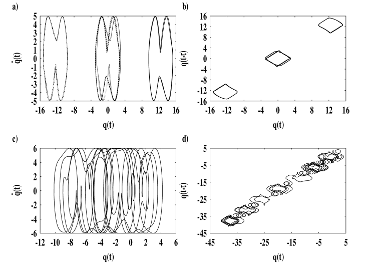
Figure 6: Analyzing the regime $R>4.90$: a,b) $R=4.95$, c,d) $R=6$.

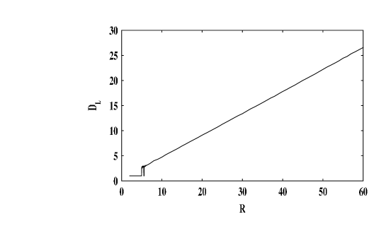
Figure 7: Lyapunov dimensions of the chaotic attractors increasing linearly with the effective control parameter $R$.

V Conclusion

Here we have demonstrated by the example of the phase–locked loop with time delay that an adequate combination of different analytical and numerical investigation methods reveals different aspects of the rich dynamical behavior in time–delayed nonlinear systems. The multiple scaling method allows to derive the normal form for the Hopf bifurcation. Phase portraits resulting from different initial functions are capable of detecting the splitting of a limit cycle indicating thereby symmetry–breaking bifurcations. A period–doubling is qualitatively indicated in the power spectrum, whereas the Lyapunov spectrum allows more quantitative statements. In this way we found within the numerical accuracy evidence that the period–doubling scenario in the phase–locked loop with time delay is governed by the Feigenbaum constant $\delta\approx 4.669$.

VI Acknowledgment

We cordially thank the anonymous referee for his suggestions to improve the manuscript. In addition, we thank Hermann Haken and Arne Wunderlin for teaching us synergetics for many years as well as Wolfgang Wischert for introducing us to dynamical systems with time delay a decade ago. Furthermore, we are thankful to Elena Grigorieva for sharing her knowledge on the multiple scaling method. Finally, A.P. is grateful for the hospitality of Günter Wunner at the I. Institute of Theoretical Physics at the University of Stuttgart as this article was finished there.

References

- (1) Y. Cho and T. Umeda, Opt. Comm. 59, 131 (1986).
- (2) E.V. Grigorieva, S.A. Kashchenko, N.A. Loiko, and A.M. Samson, Physica D 59, 297 (1992).
- (3) L. Glass and M.C. Mackey, Science 197, 287 (1977).
- (4) M.C. Mackey, Bull. Math. Biol. 41, 829 (1979).
- (5) J. Bélair and M.C. Mackey, J. of Dyn. and Diff. Eq. 1, 299 (1989).
- (6) M.C. Mackey, J. of Econ. Theory 48, 497 (1989).
- (7) J.M. Cushing, Integrodifferential Equations and Delay Models in Population Dynamics, Vol. 20 of the series Lecture Notes in Biomathematics, Springer (1977).
- (8) K. Gopalsamy, Stability and Oscillations in Delay Differential Equations of Population Dynamics, Kluwer (1992).
- (9) A. Namajunas, K. Pyragas, and A. Tamasevicius, Phys. Lett. A 204, 255 (1995).
- (10) K. Pyragas, Phys. Lett. A 170, 421 (1992).
- (11) K. Pyragas and A. Tamasevicius, Phys. Lett. A 181, 99 (1993).
- (12) E. Ott, C. Grebogi, and J.A. Yorke, Phys. Rev. Lett. 64, 1196 (1990).
- (13) W. Wischert, A. Wunderlin, A. Pelster, M. Olivier, and J. Groslambert, Phys. Rev. E 49, 203 (1994).
- (14) P. Tass, A. Wunderlin, and M. Schanz, J. Biol. Phys. 21, 83 (1995).
- (15) J.K. Hale, Theory of Functional Differential Equations, Springer (1997).
- (16) N. Krasovskii, Stability of Motion, Stanford University Press (1963).
- (17) H. Haken, Synergetics – An Introduction, Third and Enlarged Edition, Springer (1983).
- (18) H. Haken, Advanced Synergetics, Corrected Second Printing, Springer (1987).
- (19) H. Haken, Information and Selforganization, Springer (1988).
- (20) H. Haken, Synergetic Computers and Cognition, Springer (1991).
- (21) H. Haken, Principles of Brain Functioning, Springer (1996).
- (22) J.E. Marsden and M. McCracken, The Hopf Bifurcation and Its Applications, Vol. 19 of the Series Applied Mathematical Sciences, Springer (1976).
- (23) J. Guckenheimer and P. Holmes, Nonlinear Oscillations, Dynamical Systems and Bifurcations of Vector Fields, Vol. 42 of the series Applied Mathematical Sciences, Springer (1993).
- (24) R.H. Rand and D. Armbruster, Perturbation Methods, Bifurcation Theory and Computer Algebra, Vol. 65 of the series Applied Mathematical Sciences, Springer (1987).
- (25) M. Schanz, Zur Analytik und Numerik zeitlich verzögerter synergetischer Systeme, PhD thesis (in German), Universität Stuttgart, Shaker (1997).
- (26) J. Kevorkian, in Space Mathematics III, Lectures in Applied Mathematics 7, Amer. Phys. S. (1966), p. 206.
- (27) W. Lick, SIAM J. Appl. Math. 17, 815 (1969).
- (28) A. Wunderlin and H. Haken, Z. Phys. B 21, 393 (1975).
- (29) C.M. Bender and S.A. Orszag, Advanced Mathematical Methods for Scientists and Engineers – Asymptotic Methods and Perturbation Theory (McGraw-Hill, New York, 1978).
- (30) P. Manneville, Dissipative Structures and Weak Turbulence (Academic Press, Inc., San Diego, 1990).
- (31) E. Grigorieva, H. Haken, S.A. Kashchenko, and A. Pelster, Physica D 125, 123 (1999).
- (32) W.M. Wright, J. Reine Angew. Math. 194, 66 (1955).
- (33) M. Schanz and A. Pelster, accepted for publication in: SIAM Journal on Applied Dynamical Systems. eprint: nlin.CD/0203005,
- (34) M. Schanz and A. Pelster, On the Period–Doubling Scenario in Dynamical Systems with Time Delay, Proceedings of the 15th IMACS World Congress on Scientific Computation, Modelling and Applied Mathematics, Berlin, August 24–29, 1997, Wissenschaft und Technik Verlag, Vol. 1, 215 (1997).
- (35) C. Simmendinger, Untersuchung von Instabilitäten in Systemen mit zeitlicher Verzögerung, diploma thesis (in German), Universität Stuttgart (1997).
- (36) A. Wolf, J.B. Swift, H.L. Swinney, and J.A. Vastano, Physica D 16, 285 (1985).
- (37) J.D. Farmer, Physica D 4, 366 (1982).
- (38) S. Grossmann and S. Thomae, Z. Naturforsch. A 32, 1353 (1977).
- (39) M.J. Feigenbaum, J. Stat. Phys. 19, 25 (1978).
- (40) M. Le Berre, E. Ressayre, A. Tallet, H.M. Gibbs, D.L. Kaplan, and M.H. Rose, Phys. Rev. A 35, 4020 (1987).
- (41) V. Avrutin, R. Lammert, M. Schanz and G. Wackenhut, AnT 4.669: A Tool for Simulating and Investigating Dynamical Systems. submitted to: SIAM Journal of Scientific Computing
-
(42)
AnT 4.669: A software package for simulating and analyzing dynamical
systems. University of Stuttgart, 2002
http://www.AnT4669.de
The Poincaré sections of Fig. 3 in section IV were obtained by using this software package which is designed for the simulation and analysis of non–linear dynamical systems belonging to various classes, for instance maps, ordinary, delay and functional differential equations, as well as many sub–classes derived from these. AnT 4.669 supports the investigation of their dynamic behavior with several provided investigation methods, like for instance period analysis, Lyapunov exponents calculation or the generalized Poincaré section analysis and much more. Another feature of AnT 4.669 is the ability to investigate a dynamical system by varying some relevant influence quantities, such as the control parameters, initial values, or even some parameters of the investigation methods. The calculations which are necessary to perform such one, two or even higher dimensional scans can be easily distributed among several nodes of a cluster or grid using a client server architecture.