Polymer dynamics in chaotic flows with strong shear component

Abstract

We consider the internal dynamics of the polymer molecule which is injected in the chaotic flow with strong mean shear component. The flow geometry corresponds to the recent experiments on the elastic turbulence (Groisman, Steinberg 2000). The passive polymer in such flows experiences aperiodic tumbling. We present a detailed study of the statistical properties of such polymer dynamics. First we obtain the stationary probability distribution function of the polymer orientation. Secondly we find the distribution of the time periods between consequent events of tumbling, and finally we find the tails of the polymer size distribution.

Hydrodynamics and rheology of dilute polymer solutions has attracted much theoretical and experimental attention recently. Addition of small amount of polymers to ordinary liquid leads to crucial changes of liquid properties. One of the most famous effects of this type is the phenomenon of drag reduction. The addition of few parts per million of long-chain polymer molecules produces a dramatic reduction of the friction drag. Although this effect was first observed by Toms in 1949 Toms , there is still no rigorous theory, explaining the phenomena. The qualitative description was proposed by Lumley Lumley1 ; Lumley2 , but no quantitative theory is available. Another spectacular phenomena, observed in dilute polymer solutions is the effect of elastic turbulence, discovered recently by Groisman and Steinberg 00GS ; 04GS . In this experiment a chaotic fluid motion was observed in the system with small Reynolds number ${\rm Re}\ll 1$. Obviously, such behavior can not be observed in Newtonian liquids, where the flow should be laminar, so the chaotic flow is generated by the elastic instabilities of polymer solution. The dynamics of polymers and possible mechanisms, explaining the chaotic state were studied in the recent theoretical works 00BFL ; 00Che ; 03FL . It was proposed that elastic instabilities occur because of elongation of a single polymer in external flows. The analysis of the single polymer dynamics in chaotic flows, shows that the transition between two qualitatively different types of behavior of polymers can be observed in such system. This transition is called coil-stretch transition. It separates the dynamics in weak flows, where polymer molecules remain in coiled state most of the time, and strong flows, where the molecules become substantially elongated. The measure of the flow strength is given by the Weissenberg number which is the product of the characteristic velocity gradient and the polymer relaxation time. More precisely the Weissenberg number is defined as ${\rm Wi}=\lambda\tau$, where $\lambda$ is the largest Lyapunov exponent, associated with the flow, and $\tau$ is the relaxation time of the slowest polymer excitation mode. The coil-stretch transition occurs at ${\rm Wi}=1$. With the development of novel optical methods a number of high quality experimental observations focusing on resolving dynamics of individual polymers (DNA molecules) subjected to a non-homogeneous flow have been reported 97PSC ; 98SC ; 99SBC ; 01HSBSC . It made possible the direct observation of coil-stretch transition 04GCS . However in all theoretical works, describing the polymer dynamics in chaotic flows one of the important assumptions was the isotropic statistics of the velocity field. At the same time in the experiments on elastic turbulence the flow consists of regular (shear-like) and chaotic components, the latter is relatively weak in comparison with the former one. Thus, it became an important task to generalize the known theoretical results on the flows of such type.

In this paper we study the dynamics of the DNA polymers injected in the chaotic flow. The flow consists of large stationary shear component with the small chaotic part. It is assumed that the concentration of the injected polymers is small enough so that their back reaction on the flow is negligible. It was shown in 04CKLT that the polymer spends most of the time stretched in the shear direction and experiences aperiodic tumbling towards the opposite direction. The main aim of this paper is to present a detailed investigation of the statistical properties of such polymer dynamics and to make some predictions which can be checked experimentally. First, we obtain the exact expression of the polymer direction distribution. We show that the body of the angular distribution function is located in the region of small angles, which correspond to the polymer stretched in the shear direction. However, the tails of the PDF are algebraic, so the fluctuations of the polymer direction are very strong. Secondly we study the statistics of the time periods between consequent events of polymer tumbling. It is shown that this PDF has an exponential tail at large tumbling times, and two different asymptotic regimes in the region of very small times. Finally, for polymers, which are below the coil-stretch transition we obtain the asymptotic of the polymer size distribution function, which is also algebraic. We also show, that mean-shear component leads to a significant broadening of the polymer size distribution. This effect is surprising at the first sight, because the shear component itself doesn’t lead to an exponential polymer growth, and thus can not lead to the algebraic tails of the polymer size distribution. However the combined effect of the strong regular shear and chaotic velocity components leads to a significant enhancement of the polymer growth rate.

The overall plan of this article is following: in first section we describe the experimental setup in which the elastic turbulence is observed, then we discuss the assumptions of the models, describing internal polymer dynamics and flow statistics. In the main sections we give the detailed analysis of the polymer dynamics, including the tumbling phenomenon 04CKLT and statistical properties of polymer elongation. While in this paper we present only analytical predictions, some of them have been successfully checked numerically in other paper alb .

I Experimental setup

The classical effect of well-developed turbulence is observed in the systems with large values of Reynolds number ${\rm Re}=VL/\nu\gg 1$, where $V$ is the characteristic value of the flow velocity, $L$ is the characteristic system size, and $\nu$ is kinematic viscosity. In this case the chaotic motion is generated by the large nonlinear terms in the Navier-Stokes equation frisch . In the recently discovered elastic turbulence phenomena the chaotic behaviour is observed at extremely small Reynolds numbers ${\rm Re}\ll 1$, and is due to elastic instabilities of the polymer solution. The experimental setup in which this effect has been observed looks as following: a swirling flow is generated between two coaxial disks of the radius $R$ and with the gap $d\ll R$. The upper disk is being rotated with the angular frequency $\Omega$, while the lower one is stationary. For small frequencies or usual Newtonian liquid the following laminar stationary flow will be generated:

$$V_{\phi}=\Omega rz/d,\qquad V_{r}=V_{z}=0,$$ (1)

Here $\phi,z,r$ are the usual cylindrical coordinates with the center coinciding with the center of the lower disk. In the dilute polymer solution a small chaotic component of the velocity field $v$ appears after some critical value of $\Omega$ (but still at small Reynolds numbers). Currently existing theoretical works are unable to describe the statistical properties of such flow. Thus, it is of interest to study this properties experimentally. One of the experimental possibilities of such study is the observation of dynamics of single long polymer molecule (such as DNA). It should be stressed, that the observed molecules are not related to the polymers, which are dissolved in the liquid, and which generate the chaotic flow. The concentration of the observed DNA molecules is negligibly small, so they can be treated as passive objects. In the following text we won’t analyze the origins of the elastic turbulence, and will denote by the polymers the passive observed DNA molecules.

II Polymer and chaotic flow models

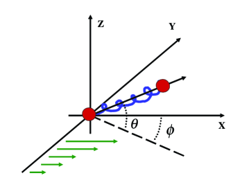
Figure 1: Schematic figure explaining polymer orientation geometry.

For typical polymers the inertial effects can be neglected, and one can assume that the polymer simply follows the lagrangian trajectories of the velocity field. In this case the velocity field affects the internal polymer dynamics in two ways: firstly the local velocity gradients lead to the polymer stretching and rotation, secondly, if the flow parameters are spatially inhomogeneous (which happens for example in the experimental setup described above), the lagrangian advection can lead to the time dependent local velocity gradients, corresponding to the stationary velocity component. In our analysis we neglect the second effect. In the case of the elastic turbulence experimental setup described above, the advection in the radial direction, which leads to the variations of the local shear rate is determined only by the chaotic component which is assumed to be small. It means the that significant changes of the local shear rate, due to lagrangian advection occur on the time scales, much larger than the characteristic time scales associated with the internal polymer dynamics. Therefore in the adiabatic approximation one can assume the local shear rates, correposding to the regular velocity component to be constant. Polymer extension can be described by the simple dumb-bell model, where the end-to-end separation vector R satisfies the following equation Hinch ; book :

$$\partial_{t}R_{i}=R_{j}\nabla_{j}v_{i}-\gamma(R)R_{i}+\zeta_{i}$$ (2)

where the relaxation rate $\gamma$ is the function of the absolute value $R$ of the vector ${\bf R}$, the velocity gradient $\nabla_{j}v_{i}$ is taken at the molecule position, and $\zeta_{i}$ is the thermal Langevin force. We assume that velocity field is large-scale, so it can be assumed to be smooth on the polymer size. This assumption justifies, the linear approximation of the velocity field used in (2). In this paper we discuss two different situations. Firstly when the Lyapunov exponent, corresponding to the velocity field is larger than the polymer relaxation rate, so the coil-stretch transition has already occurred, the polymer becomes nonlinearly stretched so, one can neglect the thermal forces $\zeta_{i}$ acting on him 00BFL . One can introduce the polymer direction vector $n_{i}=R_{i}/R$, which is in this case described by the following equation:

$$\partial_{t}n_{i}=n_{j}(\delta_{ik}-n_{i}n_{k})\nabla_{i}v_{k}$$ (3)

One can see that the direction evolution is completely decoupled from the dynamics of the polymer size $R$. In the second situation beyond the coil-stretch transition, one can not neglect the thermal force $\zeta_{i}$ and the dynamics of the polymer direction becomes more complicated. We will study only the statistics of the polymer size $R$ in this case. If the average polymer size is much smaller than it’s nonlinear length, one can assume the relaxation $\gamma(R)$ to be constant, in which case the equation (2) becomes constant and can be easily analyzed.

Next, it is important to discuss how the chaotic velocity component is modeled. The statistical properties of the velocity field, observed in the chaotic turbulence are not known neither from the experimental nor theoretical points of view. In this paper we will study the simplest model when the velocity field consists of the strong stationary shear component and of the weak short correlated chaotic component. Under this assumptions the velocity gradient matrix has the following form:

$$\nabla_{j}v_{i}=s\delta_{iX}\delta_{jY}+\sigma_{ij}$$ (4)

$$\langle\sigma_{ij}(t)\sigma_{kl}(t^{\prime})\rangle=D\delta(t-t^{\prime})(4\delta_{ik}\delta_{jl}-\delta_{il}\delta_{kj}-\delta_{ij}\delta_{kl})$$ (5)

Here we assume that the shear flow occurs in the $XY$ plane (note that this plane is stationary in the rotating frame, associated with the polymer). The exact form of the correlation function (5) assumes the isotropy of velocity component, however as we will see this assumption is not important, because in the case of strong shear component $s\gg D$ the polymer spends most of the time stretched in the $X$ directions, and it’s angular dynamics is determined only by the $Y$ component of the chaotic velocity field.

In order to simplify the equations on the polymer direction we parameterize the vector ${\bf n}$ as shown in the Fig. 1. The Eq. (3) acquires the following form

$$\partial_{t}{\phi}=-s\sin^{2}\phi+\xi_{\phi}\,,$$ (6)

$$\partial_{t}{\theta}=-s\frac{\sin(2\phi)}{2}\sin\theta+\xi_{\theta}\,,$$ (7)

where $\xi_{\phi}$ and $\xi_{\theta}$ are zero mean random variables related to chaotic components of the velocity gradient. The statistics of both $\xi_{\phi}$ and $\xi_{\theta}$ can be obtained from the correlation function (5):

$$\langle\xi_{\theta}(t)\xi_{\theta}(t^{\prime})\rangle=4D\delta(t-t^{\prime})$$ (8)

$$\langle\xi_{\phi}(t)\xi_{\phi}(t^{\prime})\rangle=\frac{4D}{\cos^{2}\theta}\delta(t-t^{\prime})$$ (9)

III Statistics of polymer direction

III.1 $\phi$-angle distribution

It follows from (3) that for the stretched polymers the angular dynamics is decoupled from the dynamics of the polymer size. In the case of $s\gg D$ the regular component will play the main role in the evolution of the polymer direction. For vanishing chaotic component $D=0$ the deterministic polymer dynamics can be easily analyzed: there are two semistable equilibrium states $\phi_{1,2}=0,\pi;\theta_{1,2}=0$, and the polymer direction vector ${\bf n}$ asymptotically approaches one of these points depending on it’s initial orientation. However when the angle between polymer and equilibrium direction becomes sufficiently small, the chaotic components $\xi_{k}$ can not be neglected, and the polymer dynamics becomes stochastic. After some time the chaotic component transfers the polymer into instable region, and regular velocity quickly (on times of order $s^{-1}$) transfers it to the opposite equilibrium direction. Due to stochastic nature of the chaotic velocity component one will observe random a-periodic tumbling of polymer. This phenomena was qualitatively analyzed in 04CKLT for general velocity statistics. In this work we focus on the situation where the chaotic flow is short correlated, such that it’s characteristic correlation time $\tau_{v}$ is small compared to the time scale, associated with the tumbling effect which as we will show can be estimated as $\tau_{t}=(Ds^{2})^{-1/3}\gg s^{-1}$. This assumption will allow us to obtain some rigorous results on the stationary and dynamical statistics of polymer.

When the chaotic component is weak enough $D\ll s$ the polymer spends most of the time in the stochastic regime, close to the equilibrium point, so that it’s angles are small $\theta,\phi\ll 1$ (we will analyze only one equilibrium point, because of the symmetry ${\bf n}\to-{\bf n}$). In this case one can set $\theta=0$ in the correlation function (9), so the dynamics of angle $\phi$ becomes decoupled from everything else, and one can write the corresponding Fokker-Planck equation:

$$\left[\partial_{t}-s\partial_{\phi}\sin^{2}\phi-2D\partial_{\phi}^{2}\right]P(t,\phi)=0$$ (10)

One of the important questions that should be discussed here are the boundary conditions, that should be used with this equation. The equation is invariant under the transformations $\phi\to\phi\pm\pi$. Therefore it would be natural to use periodic boundary conditions $P(t,-\pi/2)=P(t,\pi/2)$. In this case there will exist an asymptotic stationary solution of (10) $P_{st}(\phi)$. Obviously, all angles differing to the value divisible by $\pi$ are identical to each other in this solution. Another possibility is to use traditional boundary conditions ${\cal P}(t,\infty)={\cal P}(t,-\infty)=0$. In this case the angles $\phi$ and $\phi+\pi k$ are not equivalent, and one can study the statistics of the number of polymer rotations. The main disadvantage of such approach is that there is no stationary solution of the Fokker-Planck equation, because the PDF is widening and drifting constantly. However both of the approaches lead to the same physical results, the following identity holds between two different PDFs:

$$P(t,\phi)=\sum_{k}{\cal P}(t,\phi+\pi k)$$ (11)

In order to find the stationary PDF $P_{st}(\phi)$ we rewrite the Fokker-Planck equation in the following form:

$$\partial_{\phi}U^{-1}(\phi)\partial_{\phi}U(\phi)P_{st}(\phi)=0$$ (12)

$$U(\phi)=\exp\left[\frac{s}{4D}\phi-\frac{s}{8D}\sin 2\phi\right]$$ (13)

Trivial integration leads to the following expression for PDF:

$$P_{st}(\phi)=\frac{\omega}{D}\int_{0}^{\pi}\mathrm{d}\phi\exp\left[-\frac{s}{4D}\left(\phi-\sin\phi\cos(\phi-2\phi)\right)\right],$$ (14)

where $\omega$ is the average rotation frequency of the polymer, which is determined from the normalization condition $\int_{0}^{\pi}P_{st}(\phi)\mathrm{d}\phi=1$ and is given by

$$\omega=\frac{D\exp\left(\frac{\pi s}{8D}\right)}{\pi^{2}I_{ix}(x)I_{-ix}(x)},$$ (15)

where $x=s/8D$. In the most interesting case $s\gg D$, the PDF will be localized at small angles $\phi\sim(D/s)^{1/3}\ll 1$ and all expressions are significantly simplified:

$$\omega=\frac{(Ds^{2})^{1/3}}{4\cdot 3^{1/6}\Gamma(7/6)\sqrt{\pi}}$$ (16)

$$P_{st}(\phi)=\frac{\omega}{D}\int_{0}^{\infty}\mathrm{d}\phi\exp\left[-\frac{s}{8D}\phi(\phi-2\phi)^{2}-\frac{s\phi^{3}}{24D}\right]$$ (17)

One can see, that the PDF is asymmetric and has wide algebraic tails:

$$\langle\phi\rangle=\left(\frac{D}{s}\right)^{1/3}\frac{\sqrt{\pi}3^{1/3}}{\Gamma(1/6)}$$ (18)

$$P_{st}(\phi)\sim\frac{1}{16\cdot 3^{1/6}\Gamma(7/6)\sqrt{\pi}}\left(\frac{s}{D}\right)^{2/3}\frac{1}{\phi^{2}},$$ (19)

where the last asymptotic is valid in the intermediate region $(D/s)^{1/3}\ll|\phi|\ll 1$ The asymptotic $P_{st}\propto\phi^{-2}$ corresponds to the non-zero probability flux at $|\phi|\to\infty$ which is a manifestation of the described above tumbling effect. Positive value of the average angle $\phi$ shows, that the polymer spends most of the time in the region $\phi>0$ in agreement with the qualitative analysis presented in the first sections of this paper. One can see, that the polymer spends most of the time in the region of small angles, therefore the only relevant velocity component $v_{z}$. The assumption of isotropic statistics of chaotic velocity component is not therefore significant for the qualitative results of this paper.

III.2 Tumbling time statistics

In this section we will calculate the probability distribution function of the time intervals between consequent tumblings. Such PDF can be directly measured experimentally. For this problem it is naturally to use the non-stationary PDF ${\cal P}(t,\phi)$. We will define the tumbling process by a polymer direction “trajectory” starting at $\phi=\pi/2$ and reaching $\phi=-\pi/2$ at time $T$. In this case the probability of finding the polymer inside this region is given by

$$p(t)=\int_{-\pi/2}^{\pi/2}{\cal P}(t,\phi)\mathrm{d}\phi.$$ (20)

Where the initial condition is ${\cal P}(t,\phi)=\delta(\phi-\pi/2+0)$, so $p(0)=1$. We substitute ${\cal P}(t,\phi)=U^{1/2}(\phi)\Psi(t,\phi)$. In this case the evolution of $\Psi$ is determined by the one-dimensional Schroedinger equation in imaginary time:

$$\partial_{t}\Psi=-\hat{H}\Psi$$ (21)

$$\hat{H}=-2D\partial_{\phi}^{2}+\frac{s^{2}}{8D}\sin^{4}\phi-s\sin\phi\cos\phi$$ (22)

Now it is possible to use the quantum-mechanical analogy. The hamiltonian $\hat{H}$ formally describes a particle in periodic potential with the period $\pi$. General solution of this problem looks like

$$\Psi(t,\phi)=\sum_{n}\int\mathrm{d}p\Psi_{np}(\phi)\Psi_{np}^{*}(\pi/2)\exp(-E_{n}(p)t),$$ (23)

where $p$ is particle’s quasimomentum, and index $n$ enumerates the Brillouin zone number. In this potential the classical minimums are separated by large barriers. And for $s\gg D$ one can use the tight-binding method abrikosov . The following approximate relations hold for the spectrum:

$$E_{n}(p)=\epsilon_{n}-\nu\cos(\pi p)$$ (24)

$$\Psi_{np}(\phi)=\sum_{k}\exp(i\pi kp)\psi_{n}(\phi-k\pi),$$ (25)

where $\psi_{n},\epsilon_{n}$ is the spectrum, which is formed near classical minimums, when the tunneling processes are neglected. $\nu$ is exponentially small band width. Therefore at large times the main asymptotic of $p(t)$ will be determined by the ground state energy $\epsilon_{0}$:

$$p(t)\propto\exp(-\epsilon_{0}t),\qquad t\to\infty$$ (26)

One can easily check that this energy is given by $\epsilon_{0}=c(Ds^{2})^{1/3}$, where $c$ is a constant of order unity. Indeed, the classical minima is situated in the region of small angles $|\phi|\ll 1$, so one can use Taylor expansions of trigonometric functions. After the substitution $\phi=(D/s)^{1/3}$ one obtains the Hamiltonian

$$\hat{H}=(Ds^{2})^{1/3}\left[-2\partial_{x}^{2}+\frac{x^{4}}{8}-x\right].$$ (27)

The operator in square brackets contains no dimensionless parameters, and therefore it’s eigenvalues will be of order unity. The body of the PDF is also situated in the region of tumbling periods of order $T\sim(Ds^{2})^{-1/3}$. Left tail of tumbling time PDF $T\ll(Ds^{2})^{-1/3}$ is determined by rare trajectories, which turn the polymer by angle $\pi$ at small times $T$. In order to find the optimal form of such trajectories we will functional integral representation of the transition probability

$$p(T)\propto\int{\cal D}\phi\exp\left[-\frac{1}{8D}\int\mathrm{d}t(\dot{\phi}+s\sin^{2}\phi)^{2}\right]$$ (28)

The integration is taken over trajectories with boundary conditions $\phi(0)=\pi/2,\phi(T)=-\pi/2$. For small $T\ll(Ds^{2})^{-1/3}$ the probability is determined by the action $A$ on the optimal trajectory $p(T)\sim\exp(-A)$ with exponential accuracy. Variation of the effective action leads to the following equation on instanton:

$$\ddot{\phi}=s^{2}\sin^{3}\phi\cos\phi$$ (29)

This mechanical problem can be easily solved, and one obtains the following relation between the tumbling time and effective particle energy:

$$T=\int_{-\pi/2}^{\pi/2}\frac{\mathrm{d}\phi}{\sqrt{2E+s^{2}\sin^{4}\phi}}=\left[\frac{8}{E(2E+s^{2})}\right]^{1/4}K\left(\frac{1}{2}-\sqrt{\frac{E}{4E+2s^{2}}}\right),$$ (30)

where $K(x)$ is elliptical integral of the first kind. The action in this case is given by

$$A=\frac{ET}{4D}+\frac{s^{2}}{4D}\int\mathrm{d}\phi\frac{\sin^{4}\phi}{\sqrt{2E+s^{2}\sin^{4}\phi}}=\frac{ET}{4D}+\frac{3\pi s^{2}}{32D\sqrt{2E}}\,_{3}F_{2}\left(\frac{1}{2},\frac{5}{4},\frac{7}{4};\frac{3}{2},2;-\frac{s^{2}}{2E}\right)$$ (31)

Here we omitted the constant term $2s\int\dot{\phi}\sin^{2}\phi\mathrm{d}t=\pi s/(8D)$ because it is cancelled by the normalization constant. Because of additional time scale $s^{-1}$ there are two different asymptotes of $p(t)$. In the case of $sT\ll 1$ one has $s\ll\sqrt{2E}$ and $E=\pi^{2}/(2T^{2})$. In this case

$$A=\frac{\pi^{2}}{8DT}$$ (32)

In another limiting case $s^{-1}\ll T\ll(Ds^{2})^{-1/3}$ the energy is given by $E=8K^{4}(1/2)/(s^{2}T^{4})$ and the action has the following form:

$$A=\frac{2K^{4}(1/2)}{3Ds^{2}T^{3}}$$ (33)

The intermediate asymptotic (33) is a function of the product $Ds^{2}T^{3}$ because it is determined by the dynamics in the region of small angles. Therefore it will be universal, in the sense mentioned above. In contrary, the asymptotic at the smallest times (32) does not depend on $s$ at all, because such small times can be reached only due to very rare fluctuation of chaotic velocity field. Therefore, this asymptotic strongly depends on the assumption of isotropic velocity statistics, and is not universal.

III.3 $\theta$-angle distribution

As it was shown in 04CKLT there are two contributions to the intermediate right tail of the $\theta$-angle distribution $(D/s)^{1/3}\ll\theta\ll 1$. The first one is coming from the region of deterministic regions where $\phi\sim 1$, where the angular dynamics is determined by the regular terms. The algebraic tail in this case is proportional to $\theta^{-2}$, however there is also a non-universal algebraic part, which comes from the stochastic region of $\phi\sim(D/s)^{1/3}$ and is determined by the statistical properties of the random velocity field. In this section we will be interested in this part, and will obtain the connection between the exponent and the entropy function of the random velocity process. In the region $\theta\ll 1$ the equation (7) can be easily solved:

$$\theta(t)=\int_{0}^{\infty}\mathrm{d}\tau\exp\left(-\frac{s}{2}\int_{t-\tau}^{t}\sin 2\phi(t^{\prime})\mathrm{d}t^{\prime}\right)\xi_{\theta}(t-\tau)$$ (34)

As we already know the random process $\phi(t)$ is stationary and independent from $\xi_{\theta}(t)$. In this case the expression for $\theta$ can be rewritten in the form

$$\theta=\int_{0}^{\infty}\mathrm{d}\tau\exp(-\varrho(\tau))\xi_{\theta}(\tau)$$ (35)

$$\varrho(\tau)=\frac{s}{2}\int_{0}^{\tau}\sin 2\phi(t)\mathrm{d}t$$ (36)

In order to obtain the PDF $P(\theta)$ we first average over the noise $\xi_{\theta}$:

$$P(\theta|\varrho)=(2\pi A)^{-1/2}\exp\left[-\frac{\theta^{2}}{2A}\right]$$ (37)

$$A=4D\int_{0}^{\infty}\mathrm{d}\tau\exp[-2\varrho(\tau)].$$ (38)

Here $P(\theta|\varrho)$ is the PDF of $\theta$ for a fixed realization of the process $\varrho(t)$. Due to positive value of $\langle\dot{\varrho}\rangle\sim(Ds^{2})^{1/3}$ the body of $P(\theta)$ is situated in the region of small angles $\theta\sim(D/s)^{1/3}\ll 1$. Tails of the PDF are determined by large deviations of negative $\varrho(t)$. Assuming that the process $\varrho(t)$ reaches it’s most negative value to the time $\tau^{*}$, such that $\varrho(\tau^{*})=-\varrho^{*}$ and $\rho^{*}\gg 1$ one can estimate the value of $A$ with exponential accuracy as $A\sim(D/s)^{1/3}\exp(2\varrho^{*})$. The characteristic correlation time of $\varrho(t)$ is $\tau_{c}=(Ds^{2})^{-1/3}$, so for large $\tau^{*}\gg\tau_{c}$ one can use the results of large deviations theory 85Ell which predict the following scaling for the tails of $\rho^{*}$ PDF:

$$P(\varrho^{*}|\tau^{*})=\exp\left[-\frac{\tau^{*}}{\tau_{c}}S(\frac{\varrho^{*}\tau_{c}}{\tau^{*}})\right],$$ (39)

where $S(x)$ is the entropy function, which form can not be found analytically in general case. One can now find the most probable time $\tau^{*}$ by maximizing the above probability over $\tau^{*}$. This leads one to the expression $\tau^{*}=\tau_{c}\varrho^{*}/x^{*}$, where $x$ is found from the following equation:

$$S(x^{*})=x^{*}S^{\prime}(x^{*})$$ (40)

The entropy function is of order unity, so one can expect the same from $x^{*}$. The asymptotic of $\varrho^{*}$ PDF is therefore given by

$$P(\varrho^{*})\sim\exp(-\varrho^{*}S^{\prime}(x^{*}))$$ (41)

and after averaging (37) over $\varrho^{*}$ one obtains the following asymptotic of $\theta$ PDF:

$$P(\theta)\propto|\theta|^{-S^{\prime}(x^{*})},\qquad(D/s)^{1/3}\ll|\theta|\ll 1$$ (42)

One can see that the tails are algebraic as in the case of the angle $\phi$, however the exponent is now non-universal, and depends on the statistical properties of the velocity field.

IV Statistics of polymer elongation

The tails of the polymer size PDF can be studied in the similar way as in section III.3. The explicit solution of the dynamical equation 2 in the case of linear relaxation force has the following form

$$R_{i}(t)=\int_{0}^{\infty}\mathrm{d}t\exp\left[-\gamma(t-t^{\prime})\right]W_{ij}(t,t^{\prime})\zeta_{j}(t^{\prime})$$ (43)

$$W=T\exp\left[\int_{t^{\prime}}^{t}\tilde{\sigma}(\tau)\mathrm{d}\tau\right]$$ (44)

where $\tilde{\sigma}_{ij}=\nabla_{j}v_{i}$ is the velocity gradient matrix. In order to obtain polymer size PDF we first average over the thermal Langevin force $\xi_{i}(t)$:

$$P({\bf R}|\tilde{\sigma})\propto\exp\left[-\frac{1}{2}{\bf R}^{T}I^{-1}{\bf R}\right]$$ (45)

$$I=\kappa\int_{0}^{\infty}\mathrm{d}t^{\prime}W^{T}(t^{\prime})W(t)\exp(-2\gamma t)$$ (46)

where $W(t)=W(t,0)$, and $P({\bf R}|\tilde{\sigma})$ stands for the PDF with a fixed realization of the process $\tilde{\sigma}(t)$. At large enough times $t\gg\tau_{c}$ the eigenvalues of the matrix $W^{T}W$ become widely separated and the absolute value of the end-to-end vector ${\bf R}$ is determined by the largest eigenvalue $I_{1}$:

$$P(R|\tilde{\sigma})\propto\exp\left[-\frac{R^{2}}{2I_{1}}\right]$$ (47)

It can be easily shown (see e.g. 99BF ) that for large times, when the eigenvalues $\lambda_{i}$ of $W^{T}W$ are widely separated $\lambda_{1}\gg\lambda_{2}\gg\lambda_{3}$ the dynamics of the largest one $\lambda_{1}=\exp(2\rho)$ is described by the following equation:

$$\dot{\rho}=\frac{s}{2}\cos^{2}\theta\sin 2\phi+6D+\xi_{\rho},$$ (48)

$$\langle\xi_{\rho}(t)\xi_{\rho}(t^{\prime})\rangle=2D\delta(t-t^{\prime})$$ (49)

(50)

where $\xi_{\rho}$ is obtained from the chaotic velocity correlation function (5). The eigenvalue $I_{1}$ is then given by the expression

$$I_{1}=\kappa\int_{0}^{\infty}\mathrm{d}t\exp\left[2\rho(t)-2\gamma t\right]$$ (51)

Like in the previous section $\rho(t)$ is an integral of stationary random process with the correlation time of order $\tau_{c}=(Ds^{2})^{-1/3}$, and large deviations of $I_{1}$ are determined by the large deviations of $\rho(t)$. Assuming that the integral (51) is determined by one saddle point $\tau^{*}$ and can be estimated like $I_{1}\propto\exp(2\rho^{*}-2\gamma\tau^{*})$ where $\rho^{*}=\rho(\tau^{*})$. The asymptotic of $\rho^{*}$ PDF for a fixed value of $\tau^{*}$ has the following form:

$$P(\rho^{*}|\tau^{*})\propto\exp\left[-\frac{\tau^{*}}{\tau_{c}}S_{\rho}\left(\frac{\rho^{*}\tau_{c}}{\tau^{*}}\right)\right]$$ (52)

One can now find the optimal value of $\tau^{*}=\tau_{c}\rho^{*}/x$. The coefficient $x$ is found from the following equation:

$$S_{\rho}(x)-xS_{\rho}^{\prime}(x)+\gamma\tau_{c}S_{\rho}^{\prime}(x)$$ (53)

As long as we study the linear region beneath the coil-stretch transition we have $\gamma\tau_{c}>1$. The tail of PDF will be algebraic like in case of $\theta$ angle: $P(R)\propto R^{-1-\alpha}$, and the value of $\alpha$ can be determined for large values of $\gamma\tau_{c}\gg 1$. Large deviations of $R$ are determined by the region where thermal Langevin forces can be neglected and one can use the equation (48). We are interested in the asymptotic behaviour of the polymer size moments $M_{q}(t)=\langle R^{q}(t)\rangle\propto\exp(A_{q}t)$. In this case the value of $\alpha$ will be determined from the equation $A_{\alpha}=0$. Integrating out the function $\xi_{\rho}$ one can rewrite $M_{q}$ in the following form:

$$M_{q}=\exp\left[Dq^{2}t-\gamma qt\right]\int\mathrm{d}\phi Z_{q}(\phi,t)$$ (54)

$$Z_{q}=\left\langle\exp[q\varrho(t)]\delta(\phi-\phi(t))\right\rangle$$ (55)

where the angle brackets here stand for the averaging over the process $\phi(t)$. The function $Z_{q}$ obeys the equation

$$\partial_{t}Z_{q}=\left[2D\partial_{\phi}^{2}+s\partial_{\phi}\sin^{2}\phi+\frac{qs}{2}\sin 2\phi\right]Z_{q}$$ (56)

The only difference from the Fokker-Planck equation 10 only in the last term. We will follow the same procedure as in the section III.2. Substituting $Z_{q}=U(\phi)\Psi(t,\phi)$ we obtain the imaginary time Schroedinger equation

$$\partial_{t}\Psi=-\hat{H_{q}}\Psi$$ (57)

$$\hat{H_{q}}=-2D\partial_{\phi}^{2}+\frac{s^{2}}{8D}\sin^{4}\phi+(q-1)s\sin\phi\cos\phi$$ (58)

This equation can not be solved in the case $q\sim 1$, however for $q\gg 1$ the solution can be easily found. In this case the main exponential asymptotic at large times is $Z_{q}(t)=\propto\exp(-\epsilon(q)t)$, where $\epsilon(q)$ is the ground state energy. For $q\gg 1$ the main contribution to $\epsilon(q)$ will be equal to the value of classical minima of the potential. After some simple algebra we obtain

$$\epsilon(q)\sim-3\cdot 2^{-5/3}\left(q^{4}Ds^{2}\right)^{1/3},\qquad 1\ll q\ll s/D$$ (59)

$$\epsilon(q)\sim qs/2,\qquad q\gg s/D$$ (60)

Finally we have

$$A(q)=Dq^{2}-\gamma q-\epsilon(q)$$ (61)

and the critical value $\alpha$ will depend on the dimensionless parameter $\gamma/s$:

$$\alpha=\frac{81}{32}\frac{\gamma^{3}}{Ds^{2}},\qquad\gamma\ll s$$ (62)

$$\alpha=\frac{\gamma}{D},\qquad\gamma\gg s$$ (63)

The last expression (63) coincides with the value of exponent for pure isotropic chaotic velocity, because in the case $\gamma\gg s$ large polymer size fluctuations are determined by the rare fluctuations of the chaotic component, when the flow has a strong elongation component with the lyapunov exponent $\lambda>\gamma$ for a long time. However the result (62) shows that in the case $\gamma\ll s$ the shear component can significantly broaden the tails of the polymer size PDF. This fact is nontrivial because the regular shear component itself can not lead to the exponential polymer elongation, and non-trivial exponent comes from the combined effect of chaotic and regular component.

V Conclusions

In conclusion we would like to repeat the main results of this paper. A polymer molecule injected in the chaotic flow with the strong mean shear component becomes strongly stretched in the shear direction and experiences the a-periodic tumbling in the plane of the shear flow. It is shown, that stationary distribution of the polymer orientation angles has intermediate algebraic asymptotics. The tails of the $\phi$-angle distribution behave like $\phi^{-2}$ and correspond to the constant flux solution of the Fokker-Planck equation. Existence of these asymptotics has been reported in previous papers regarding the dynamics of molecules and small particles in the shear flows book ; HinchLeal . However the algebraic asymptotic of the $\theta$-angle distribution has not been reported in any previous papers to our knowledge. We would like to stress, that in contrary to the PDF of the $\phi$ angle, the asymptotic behaviour of the $\theta$-angle distribution is not universal and depends on the statistical properties of the chaotic velocity component. Therefore in our opinion measurement of the scaling exponent of the $\theta$-angle distribution is a perfect tool for the investigation of the statistical properties of the chaotic velocity. Another quantity which can be measured by direct polymer observations is the PDF of the time periods between consequent polymer tumblings. The equilibrium direction of the polymer, which is oriented along the shear direction is semistable. This property leads to frequent polymer tumblings, so that the characteristic time between tumblings is of order $\tau\sim\tau_{c}=(Ds^{2})^{-1/3}$. The situation would be different in the case of vesicles or non-spherical particles in the shear flow HinchLeal , where the tumbling rate would be exponentially small. In the fourth part of this paper we make the prediction on the polymer size distribution. We show, that the existence of the strong shear component leads to the significant broadening of the size distribution compared to the isotropic case, which was considered in 00BFL . This effect is to our opinion rather non-trivial, because the shear component itself can not lead to the exponential elongation of the polymer and the distribution broadening is the combined effect of the chaotic and regular velocity components. Finally, we would like to mention that all results of this paper were obtained under the assumption of isotropic and short-correlated chaotic velocity flow. While the first assumption, as it was discussed throughout the paper is irrelevant for most of the results, the finite correlation time of the velocity flow can lead to the change of some quantitative results of this paper. However we believe (see 04CKLT for the more detailed discussion) that most qualitative predictions will remain valid if the velocity correlation is smaller or comparable to the characteristic time scale of the polymer dynamics $\tau_{c}$.

Author would like to thank M. Chertkov, I. Kolokolov and V. Lebedev for numerous of inspiring discussions. This work was supported by the Dynasty foundation and RFBR grant 04-02-16520a.

References

- (1) B. A. Toms, Proceedings of the International Congress of Rheology, Holland, 1948 (North-Holland, Amsterdam, 1949), pp. II-135-141
- (2) J. L. Lumley, Annu. Rev. Fluid Mech. 1, 367 (1969); J. Polymer Sci.: Macromolecular Reviews 7, 263 (1973).
- (3) J. L. Lumley, Symp. Math. 9,315 (1972)
- (4) A. Groisman and V. Steinberg , Nature 405, 53 (2000); Phys. Rev. Lett. 86, 934 (2001).
- (5) A. Groisman and V. Steinberg, New J. Phys. 6, 29 (2004).
- (6) E. Balkovsky, A. Fouxon, V. Lebedev, Phys. Rev. Lett. 84, 4765 (2000); Phys. Rev. E 64, 056301 (2001).
- (7) M. Chertkov, Phys. Rev. Lett. 84, 4761 (2000).
- (8) A. Fouxon and V. Lebedev, Phys. Fluids 15, 2060 (2003).
- (9) T. T. Perkins, D. E. Smith, and S. Chu, Science 276, 2016 (1997).
- (10) D. E. Smith and S. Chu, Science 281, 1335 (1998).
- (11) D. E. Smith, H. P. Babcock, and S. Chu, Science 283, 1724 (1999).
- (12) J. S. Hur, E. Shaqfeh, H. P. Babcock, D. E. Smith, S. Chu, J. Rheol, 45, 421 (2001).
- (13) S. Gerashchenko, C. Chevallard, and V. Steinberg, Single polymer dynamics: coil-stretch transition in a random flow, Submitted to Nature.
- (14) M. Chertkov, I. Kolokolov, V. Lebedev, K. Turitsyn, Tumbling of polymers in random flow with mean shear, Submitted to J. Fluid Mech.
- (15) A. Puliafito, K. Turitsyn, Single polymer dynamics in shear flow, In preparation.
- (16) U. Frisch, Turbulence: the Legacy of A. N. Kolmogorov, Cambridge University Press, New York (1995).
- (17) E. J. Hinch, Phys. Fluids, 20, S22 (1977)
- (18) R. B. Bird , C. F. Curtiss , R. C. Armstrong, and O. Hassager, Dynamics of Polymeric Liquids, Wiley, New York, 1987.
- (19) A. A. Abrikosov, “Fundamentals of the Theory of Metals”, North-Holland (1988)
- (20) R. Ellis, Entropy, Large Deviations and Statistical Mechanics, Springer-Verlag, Berlin, 1985.
- (21) E. Balkovsky and A. Fouxon, Phys. Rev. E 60, 4164 (1999);
- (22) E. J. Hinch, Phys. Fluids, 20, S22 (1977).
- (23) M. Chertkov and V. Lebedev, Phys. Rev. Lett 90, 034501 (2003); 90, 134501 (2003).
- (24) H. Goldsmith and J. Marlow, Proc. R. Soc. (London) B 182, 351 (1972).
- (25) S. R. Keller and R. Skallak, J. Fluid Mech. 120, 27 (1982).
- (26) J. S. Hur, E. Shaqfeh, R. G. Larson, J. Rheol. 44, 713 (2000).
- (27) E.J. Hinch, L.G. Leal (1972) in J. Fluid Mech. 52, 683-712