Logarithmically modified scaling of temperature structure functions in thermal convection

Abstract

Using experimental data on thermal convection, obtained at a Rayleigh number of 1.5 $\times 10^{11}$, it is shown that the temperature structure functions $\langle\Delta T_{r}^{p}\rangle$, where $\Delta T_{r}$ is the absolute value of the temperature increment over a distance $r$, can be well represented in an intermediate range of scales by $r^{\zeta_{p}}\varphi(r)^{p}$, where the $\zeta_{p}$ are the scaling exponents appropriate to the passive scalar problem in hydrodynamic turbulence and the function $\varphi(r)=1-a(\ln r/r_{h})^{2}$. Measurements are made in the midplane of the apparatus near the sidewall, but outside the boundary layer.

A deep similarity between statistical properties of turbulent passive scalar fluctuations sa and those of temperature fluctuations in the turbulent thermal convection kad has been discovered recently from numerical simulations (see, for instance, refs. ching1 ,biskamp and the literature cited therein). In the present note, we will use experimental data and a brief theoretical reasoning to go further in this same direction.

We consider turbulent convection in a confined container of circular crosssection and 50 cm diameter. The aspect ratio (diameter/height) is unity. The sidewalls are insulated and the bottom wall is maintained at a constant temperature, which is slightly higher than that of the top wall. The working fluid is cryogenic helium gas. By controlling the temperature difference between the bottom and top walls, as well as the thermodynamic operating point on the phase plane of the gas, the Rayleigh number ($Ra$) of the flow could be varied between $10^{7}$ and $10^{15}$. We measure the temperature fluctuations $T(t)$ at various Rayleigh numbers towards the upper end of this range, in which the convective motion is turbulent. The results used in this paper correspond mainly to $Ra=1.5\times 10^{11}$. Time traces of fluctuations are obtained at a distance of 4.4 cm from the sidewall on the center plane of the apparatus. This position is outside of the boundary layer region for the Rayleigh numbers considered here. More details of the experimental conditions and measurement procedure can be found in ref. NS1 .

For the structure functions $\langle\Delta T_{\tau}^{p}\rangle$, where the absolute values of temperature increment $\Delta T|T(t+\tau)-T(t)|$ is evaluated as a function of the time interval $\tau$ and the angle brackets indicate time averaging, we do not observe any clear scaling (see fig. 1). However, the normalized structure functions show unambiguous scaling as

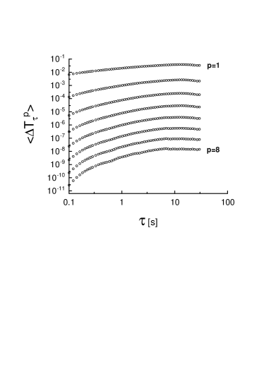
Figure 1: Temperature structure functions $\langle\Delta T_{\tau}^{p}\rangle$ against $\tau$ (in log-log coordinates). Here and for other figures, $Ra=1.5\times 10^{11}$.

$$S_{p}(\tau)=\frac{\langle\Delta T_{\tau}^{p}\rangle}{\langle\Delta T_{\tau}^{2}\rangle^{p/2}}\sim\tau^{-z_{p}}$$

(see fig. 2). The scaling exponents $z_{p}$, extracted as slopes of the best straight-line fits shown in fig. 2 (the scaling range is from $0.1$s to $10$s), indicate multiscaling. These exponents are shown in fig. 3 as circles.

It should be noted that temperature structure functions in thermal convection were investigated in ref. ching2 using the experimental data described in sano . In particular, the data used in ching2 were obtained at the center of the convection cell. While the structure functions $\langle\Delta T_{r}^{p}\rangle$ themselves showed no scaling properties, two scaling ranges were observed for the normalized structure functions $S_{p}(\tau)$. In the present paper, we study the data obtained near sidewall (see above), where sufficiently strong convection wind is present. For this case, we observe only one scaling interval for $S_{p}(\tau)$.

Since, for a passive scalar $\Theta$ advected and diffused by hydrodynamic turbulence, the scaling of structure functions follows (in both experiments and direct numerical simulations) the relation

$$\langle\Delta\Theta_{\tau}^{p}\rangle\sim\tau^{\zeta_{p}},$$

the corresponding exponents of the normalized structure functions can be readily calculated from the definition as

$$z_{p}=\zeta_{p}-\frac{p}{2}\zeta_{2}.$$

We also show in fig. 3 the values of $z_{p}$, calculated using equation (4), for the passive scalar measured in the atmosphere schmidt (inverted triangles) and from a direct numerical simulation of three-dimensional homogeneous isotropic turbulence wg (upright triangles). They are virtually indistinguishable from each other and from the present exponents extracted for thermal convection from fig. 2.

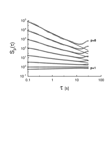
Figure 2: Normalized temperature structure functions $\langle\Delta T_{\tau}^{p}\rangle/\langle\Delta T_{\tau}^{2}\rangle^{p/2}$ against $\tau$ (in log-log coordinates). Straight lines (the best fits) are drawn to indicate the multiscaling (2).

Noting this good correspondence between $z_{p}$ for thermal convection and for the passive scalar, and further that there is no scaling of unnormalized structure functions in convection, we suggest that the structure functions $\langle\Delta T_{\tau}^{p}\rangle$ in convection should have the general non-scaling form

$$\langle\Delta T_{\tau}^{p}\rangle\sim\tau^{\zeta_{p}}\varphi(\tau)^{p},$$

where the exponents $\zeta_{p}$ are taken from the passive scalar problem. This suggestion is completely consistent with the experimentally observed multiscaling properties (2)-(4) (fig. 3). One can find $\varphi(\tau)$ explicitly from the data by dividing $\langle\Delta T^{p}_{\tau}\rangle$ by $\tau^{\zeta_{p}}$ and taking the $p$-th root of the resulting function. Figure 4 shows the outcome of these calculations for different values of $p$ (the calculated function $\varphi(\tau)$ is normalized by its maximum). In the semi-log scales used in the Fig. 4, the $\varphi(\tau)$ function has an essentially parabolic form given by

$$\varphi(\tau)=[1-a(\ln\tau/\tau_{h})^{2}]$$

where $a$ and $\tau_{h}$ are constants. The scatter of the data in fig. 4 needs a brief comment. The range of $\tau$ shown in the plot covers more than two decades. Although the tails (especially for large orders $p$) do not collapse perfectly, most of the data (in the range $-2<\ln\tau<2.5$, i.e. about two decades of $\tau$) possess a scatter of less than $6\%$.

The case of particular interest, corresponding to the second order, is shown in the inset to fig. 4; the arguments due to Corrsin and Obukhov my ) yield a specific value for the second order ($\zeta_{2}=2/3$ without intermittency corrections). The solid parabola (the best fit) corresponds to (6) with $a\simeq 0.04$ and $\tau_{h}\simeq 0.64s$. A slightly different choice for $\zeta_{2}$ to account for the intermittency effects shows no essential difference.

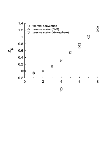
Figure 3: Scaling exponents $z_{p}$, for the normalized structure functions $S_{p}(\tau)$, extracted from fig. 2 (circles). The scaling exponents $z_{p}$ calculated using equation (4) for the passive scalar in the atmosphere schmidt (inverted triangles) and in the direct numerical simulations of mixing in three-dimensional homogeneous isotropic turbulence wg (upright triangles).

It may be useful to make the following observation. In general, for the atmosphere, the structure function data are interpreted with respect to spatial separation through the use of Taylor’s hypothesis. Because of the presence of the mean wind in the present experiment, one may use Taylor’s hypothesis my with equal facility and interpret temperature increments over time intervals as increments over equivalent spatial distances traversed by the mean wind. This hypothesis is neither critical nor necessary, though we shall use it later to be in conformity with standard practice. If the Taylor’s hypothesis is applied to temperature fluctuations in convection, one would replace the time separation $\tau$ by an equivalent spatial separation $r$, and we would have

$$\langle\Delta T_{r}^{p}\rangle\sim r^{\zeta_{p}}\cdot[1-a(\ln r/r_{h})^{2}]^{p}.$$

Local scale invariance characteristic of structure functions with scaling properties can often be interpreted, if only loosely, in terms of a conformal invariance, which may be understood as an extension of the Kolmogorov-Obukhov similarity hypothesis. There is evidence that this conformal invariance is broken for the velocity field in three-dimensional hydrodynamic turbulence lp . Equation (7) suggests the Corrsin-Obukhov scaling possesses a symmetry-breaking property (cf also mull ).

To understand the “correction” of the passive scalar scaling in (5) it is useful to consider the equations of motion in the Boussinesq approximation:

$$Pr^{-1}(\frac{\partial}{\partial t}+{\bf v}\cdot\nabla){\bf v}=-\nabla p+T\hat{z}+Ra^{-1/2}\nabla^{2}{\bf v}$$

$$(\frac{\partial}{\partial t}+{\bf v}\cdot\nabla)T=Ra^{-1/2}\nabla^{2}T$$

$$\nabla\cdot{\bf v}=0.$$

Here ${\bf v}$ and $p$ are the velocity and pressure fields, $\hat{z}$ is a unit vector in the vertical direction and $Pr$ is the Prandtl number. We expect that the anisotropy related to the thermal origin of velocity fluctuations is diminished in the inertial range of scales with $Ra\rightarrow\infty$ and so may regard, for large $Ra$, the temperature fluctuations in the spirit of a “perturbation” over the passive scalar problem.

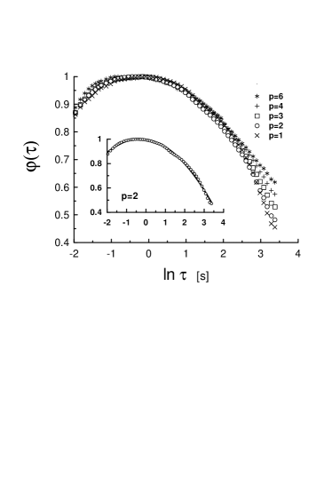
Figure 4: The function $\varphi(\tau)$ in semi-log scales. The solid parabola indicates equation (6).

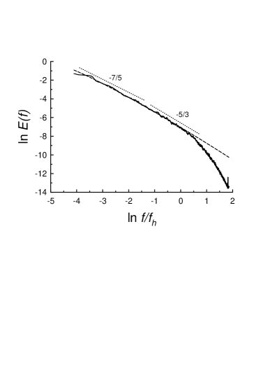
Figure 5: The spectral density of the temperature fluctuation (solid curve) against normalized frequency (in log-log coordinates). The dashed curve corresponds to the logarithmically corrected Corrsin-Obukhov spectrum (12) and dotted straight lines indicate the Bolgiano-like form $E(f)\sim f^{-7/5}$ and the Corrsin-Obukhov form $E(f)\sim f^{-5/3}$.

Finally, we wish to address briefly the power spectrum of temperature fluctuations. There is no simple way of relating the form (7) for the second-order structure function to a similarly neat form for the spectrum. However, considering that the correction to scaling presumably has its origin in a perturbation theory, we will use the same form as (7) for the spectrum as well, and replace $r$ by $k^{-1}$ (where $k$ is wave number) to write

$$E(k)\sim k^{-5/3}[1-a(\ln k/k_{h})^{2}],$$

or, for the frequency spectrum,

$$E(f)\sim f^{-5/3}[1-a(\ln f/f_{h})^{2}],$$

where $f_{h}=\tau_{h}^{-1}$ and the power “$-5/3$” is the Corrsin-Obukhov scaling for the passive scalar—corresponding to $\zeta_{2}=2/3$ noted above my . Figure 5 shows the experimentally observed spectrum of the temperature fluctuations (solid curve). The logarithmically corrected Corrsin-Obukhov form (12) is shown in this figure as the dashed curve. (The fitting range, clearly seen in fig. 5, is a bit smaller than for the normalized structure functions, where a part of ”dissipation” range is also covered by the fitting.) We also indicate by dotted lines the Corrsin-Obukhov form $E(f)\sim f^{-5/3}$ and the Bolgiano-like form $E(f)\sim f^{-7/5}$, mentioned previously in the literature in relation to the turbulent thermal convection (refs. sano ,y -nssd ). However, the Bolgiano-like fit of the spectrum has no support in the second-order structure function in our case.

In conclusion, our proposal is that the temperature fluctuations in the convection problem can be treated as a “perturbation” over the passive scalar problem, and that the “correction” is of the non-scaling form shown in (7). Empirical evidence in favor of this proposal is presented. Developing this suggestion into a full-fledged theory is beyond the scope of the present article.

- (1) K.R. Sreenivasan and R.A. Antonia, Annu. Rev. Fluid Mech, 29, 435 (1997).
- (2) L. Kadanoff, Phys. Today 54, 34 (2001).
- (3) E.S.C. Ching, et al., Phys. Rev. E, 67, 016304 (2003).
- (4) D. Biskamp, K. Hallatschek, E. Schwarz, Phys. Rev. E, 63 045302, (2001).
- (5) J.J. Niemela and K.R. Sreenivasan, J. Fluid Mech. 481, 355 (2003).
- (6) E.S.C. Ching, Phys. Rev. E, 61, R33 (2000).
- (7) M. Sano, X.Z. Wu and A. Libchaber, Phys. Rev. A 40, 6421 (1989).
- (8) A.S. Monin and A.M. Yaglom, Statistical Fluid Mechanics, Vol. 2, (MIT Press, Cambridge 1975).
- (9) F. Schmidt et al., Europhys. Lett. 34, 195 (1996).
- (10) T. Watanabe and T. Cotoh, Statistics of Passive Scalar in Homogeneous Turbulence, (submitted).
- (11) V.S. L’vov and I. Procaccia, Europhys. Lett. 29, 291 (1995).
- (12) D. Muller, Phys. Rev. D, 51, 3855 (1995).
- (13) V. Yakhot, Phys. Rev. Lett. 69, 769 (1992).
- (14) S. Grossmann and V.S. L’vov, Phys. Rev. E., 47, 4161 (1993).
- (15) S. Ashkenazi and V. Steinberg, Phys. Rev. Lett, 83, 4760 (1999).
- (16) J.J. Niemela, L. Skrbek, K.R. Sreenivasan and R.J. Donnelly, Nature 404, 837 (2000).