Synchronization in networks of general, weakly nonlinear oscillators

Abstract

We present a general approach to the study of synchrony in networks of weakly nonlinear systems described by singularly perturbed equations of the type $x^{\prime\prime}+x+\epsilon f(x,x^{\prime})=0$. By performing a perturbative calculation based on normal form theory we analytically obtain an $\mathcal{O}(\epsilon)$ approximation to the Floquet multipliers that determine the stability of the synchronous solution. The technique allows us to prove and generalize recent results obtained using heuristic approaches, as well as reveal the structure of the approximating equations. We illustrate the results in several examples, and discuss extensions to the analysis of stability of multisynchronous states in networks with complex architectures.

1 Introduction

Networks of coupled oscillators are used to describe a variety of systems in science and engineering, such as Josephson junction arrays, generators in power plants, firefly populations, and heart pacemaker cells. Of particular interest are solutions in which the network, or subpopulations within the network, oscillate synchronously. The analysis of the stability of and transition to a synchronous state can be very complex and has received much attention [1, 2, 3].

Recent applications to nanoelectromechanical systems (NEMS) [4], and beam steering devices in telecommunications [5], showed that important advances can be made by studying these problems perturbatively. It is therefore essential to have appropriate mathematical tools for such an analysis. We propose a perturbative method, based on normal form techniques [6, 7, 8], which is in many respects superior to those commonly used to study synchrony in oscillator networks.

The method is intuitive and helps us distinguish between contributions to the dynamics arising from the network configuration and the internal structure of individual oscillators. Because of this it is possible to carry out calculations without having to specify the nonlinearities explicitly. Also, the approach based on normal forms is rigorous, and the validity of approximations is known a priori. On the other hand, for methods commonly used in the physics literature, mathematical justification is often non-trivial, and must be performed a posteriori [8, 9].

There are a number of other advantages that the normal form approach brings to the table. The approximating equations to the original system are obtained by examining a collection of algebraic conditions. This procedure can be formulated in an algorithmic form and automated, which is of particular importance when approximations of higher order in the small parameter are needed. Computer codes for determining normal forms to any order already exist for some problems in celestial mechanics.

Standard methods, such as averaging, usually require center manifold reduction to be performed first [10]. We will show that the center manifold reduction is obtained naturally in the normal form of the equations of motion. Moreover, the change of coordinates leading to the normal form can be used to approximate the center manifold, the invariant fibration over the center manifolds, and a number of nearly conserved quantities of the equations to any order. As a result, the normal form method offers a deeper insight into the geometric structure of the approximating equations.

Related approaches can be found in the literature [11, 12]. In particular, the method of normal forms has been used in [13] to obtain reduced equations for oscillators close to a bifurcation. Our approach differs in that we do not consider only small amplitude oscillations, but general weakly nonlinear oscillators. Moreover, the coupling in the present case results in negative eigenvalues in the linear part of the vector field.

Figure 1: Globally coupled oscillators. Load parameters are rescaled with respect to the number of oscillators, so the values of load resistance, capacitance and inductance are $NR$, $C/N$ and $NL$, respectively.

In this paper we look at systems of globally coupled identical oscillators illustrated in Figure 1. This configuration is commonly used for wave generators in order to increase the output power (See e.g. [14]). When oscillators are synchronized the power of emitted waves scales as a square of the number of coupled units. Therefore, it is important to determine couplings that lead to synchronous behavior. Our analysis results in a general expression for the onset of synchronization in the network, and we recover recent results for an array of van der Pol oscillators [15] as a special case. Furthermore, we find, somewhat surprisingly, that the coupling can induce synchronous oscillations even in a network of weakly nonlinear systems which are unstable, and do not oscillate when uncoupled. The method itself can be easily extended to treat more complex networks and other types of coherent solutions. In order to keep our presentation streamlined we do not discuss these problems here.

This work is motivated by previous studies of synchrony in Josephson junction arrays [16, 17, 18, 19], where a series of junctions was shunted with an $RLC$ load (Fig. 1). Dhamala and Wiesenfeld introduced a heuristic, perturbative method in which an approximate stroboscopic map was constructed [19]. For an appropriately chosen strobing period $T$ the synchronous solution corresponds to a fixed point of this stroboscopic map, and the stability of the synchronous state can be determined from the eigenvalues of its linearization. A remarkable consequence of this approach is a unified synchronization law for capacitive and noncapacitive junctions, two cases which were believed to have different dynamics. An extension of the method, and an application to the study of synchrony in an array of van der Pol oscillators was given in [15].

The stroboscopic map approach, like most classical singular perturbation methods, consists of identifying and taming secular terms in the naive approximating solution of the weakly nonlinear system. The general structure of the reduced equation obtained using this approach is difficult to know before the calculations are carried out. On the other hand, the normal form method enables us to carry out calculations without having to specify the nonlinearity explicitly, or calculate the approximate strobing time $T$, and hence study a much broader class of problems.

The paper is organized as follows: In Section 2 we briefly review the theory of normal forms and illustrate it in the case of a van der Pol oscillator. These ideas are applied in Section 3 to compute the normal form of the equation describing a network of weakly nonlinear oscillators. The stability of the synchronous solution in this network is analyzed in Section 4. Several examples illustrating these ideas are given in Section 5. Finally, in Section 6 we discuss possible extensions of our work to different networks.

2 Normal Form Analysis

In this section we give outline the application of the method of normal forms to the analysis weakly nonlinear systems in a general setting. The method has been discussed in [7, 6], and a mathematical analysis is given in [20, 8]. Consider a weakly nonlinear ODE of the form

$${\mathbf{x}}^{\prime}=A{\mathbf{x}}+\epsilon\sum_{{\boldsymbol{\alpha}},i}c_{{\boldsymbol{\alpha}},i}{\mathbf{x}}^{\boldsymbol{\alpha}}e_{i}=A{\mathbf{x}}+\epsilon\mathbf{f}({\mathbf{x}}),$$ (1)

where ${\mathbf{x}}\in{\mathbb{R}}^{n}$, $A$ is an $n\times n$ constant matrix, and $e_{i}$ is the $i$-th unit vector. We use standard multi-index notation, so that ${\boldsymbol{\alpha}}\in{\mathbb{N}}^{n}$ and ${\mathbf{x}}^{\boldsymbol{\alpha}}=x_{1}^{\alpha_{1}}\cdots x_{n}^{\alpha_{n}}$. We emphasize that, in contrast with local normal form theory, $\mathbf{f}({\mathbf{x}})$ may contain any monomial in ${\mathbf{x}}$, including linear terms.

A goal of normal form theory is to remove terms of $\mathcal{O}(\epsilon)$ in equation 1 by a near-identity change of variables

$${\mathbf{x}}={\mathbf{y}}+\epsilon\mathbf{g}({\mathbf{y}}),\qquad\mathbf{g}:{\mathbb{R}}^{n}\rightarrow{\mathbb{R}}^{n},$$ (2)

where $\mathbf{g}({\mathbf{y}})$ is a polynomial. In terms of the new variables (1) becomes

$${\mathbf{y}}^{\prime}=A{\mathbf{y}}+\epsilon\left(\sum_{{\boldsymbol{\alpha}},i}c_{{\boldsymbol{\alpha}},i}{\mathbf{y}}^{\boldsymbol{\alpha}}e_{i}-[A,\mathbf{g}]({\mathbf{y}})\right)+\mathcal{O}(\epsilon^{2})$$ (3)

where the Lie bracket $[A,\mathbf{g}]({\mathbf{y}})$ equals $Dg({\mathbf{y}})A{\mathbf{y}}-A\mathbf{g}({\mathbf{y}})$. To remove the nonlinear terms at $\mathcal{O}(\epsilon)$ in (3), we need to solve the equation

$$[A,\mathbf{g}]({\mathbf{y}})=\sum_{{\boldsymbol{\alpha}},i}c_{{\boldsymbol{\alpha}},i}{\mathbf{y}}^{\boldsymbol{\alpha}}e_{i}.$$ (4)

Since this equation is linear in $\mathbf{g}$, it is equivalent to the finite family of equations

$$[A,g_{{\boldsymbol{\alpha}},i}]({\mathbf{y}})=c_{{\boldsymbol{\alpha}},i}{\mathbf{y}}^{\boldsymbol{\alpha}}e_{i}.$$ (5)

If $A$ is diagonal, the eigenvectors of $[A,\cdot]$ are the homogeneous polynomials, since

$$[A,{\mathbf{y}}^{\boldsymbol{\alpha}}e_{i}]=\Lambda_{{\boldsymbol{\alpha}},i}{\mathbf{y}}^{\boldsymbol{\alpha}}e_{i},$$

where

$$\Lambda_{{\boldsymbol{\alpha}},i}=\sum_{k}\alpha_{k}\lambda_{k}-\lambda_{i}=\left\langle{{\boldsymbol{\alpha}}},{\boldsymbol{\lambda}}\right\rangle-\lambda_{i},$$ (6)

and $\lambda_{i}$ are eigenvalues of matrix $A$. It follows that, if $\Lambda_{{\boldsymbol{\alpha}},i}\neq 0$, equation 5 has the solution

$$g_{{\boldsymbol{\alpha}},i}({\mathbf{y}})=\frac{c_{{\boldsymbol{\alpha}},i}}{\Lambda_{{\boldsymbol{\alpha}},i}}{\mathbf{y}}^{\boldsymbol{\alpha}}e_{i}.$$

On the other hand, if $\Lambda_{{\boldsymbol{\alpha}},i}=0$, equation 5 does not have a solution, and we say that the monomial ${\mathbf{y}}^{\boldsymbol{\alpha}}e_{i}$ is resonant. Therefore, only nonlinear monomials ${\mathbf{y}}^{\boldsymbol{\alpha}}e_{i}$ such that $\Lambda_{{\boldsymbol{\alpha}},i}\neq 0$ can be removed at first order in $\epsilon$ by a near identity coordinate change of the form 2.

In particular, we can split the nonlinearity $\mathbf{f}({\mathbf{y}})$ in 1 into a resonant part $\mathbf{f}^{\mathsf{R}}({\mathbf{y}})=\sum_{\Lambda_{{\boldsymbol{\alpha}},i}=0}c_{{\boldsymbol{\alpha}},i}{\mathbf{y}}^{\boldsymbol{\alpha}}e_{i}$ and a nonresonant part $\mathbf{f}^{\mathsf{NR}}({\mathbf{y}})=\sum_{\Lambda_{{\boldsymbol{\alpha}},i}\neq 0}c_{{\boldsymbol{\alpha}},i}{\mathbf{y}}^{\boldsymbol{\alpha}}e_{i}$, so that $\mathbf{f}({\mathbf{y}})=\mathbf{f}^{\mathsf{R}}({\mathbf{y}})+\mathbf{f}^{\mathsf{NR}}({\mathbf{y}})$. By setting $\mathbf{g}({\mathbf{y}})=\sum_{\Lambda_{{\boldsymbol{\alpha}},i}\neq 0}g_{{\boldsymbol{\alpha}},i}({\mathbf{y}})$, the change of coordinates 2 leads to the equation

$${\mathbf{y}}^{\prime}=A{\mathbf{y}}+\epsilon\mathbf{f}^{\mathsf{R}}({\mathbf{y}})+\mathcal{O}(\epsilon^{2}).$$ (7)

We emphasize that to obtain the normal form of equation 1 to $\mathcal{O}(\epsilon)$, we simply identify and remove all resonant terms, that is all monomials comprising $\mathbf{f}^{\mathsf{NR}}({\mathbf{x}})$. The preceding argument shows that this can be done at the expense of introducing terms of $\mathcal{O}(\epsilon^{2})$ into the equation. If the $\mathcal{O}(\epsilon^{2})$ terms are neglected in 7, a truncated normal form is obtained. To continue this process and obtain normal forms to higher order in $\epsilon$, it is necessary to compute the $\mathcal{O}(\epsilon^{2})$ terms that are introduced at this step explicitly. This is equivalent to the observation that the computation of a local normal form near a singular point to second order may affect the cubic terms, and the computation needs to be carried out order by order (see [9], for instance).

The following theorem shows that the truncated normal form provides a good approximation to the original equations

Theorem 1

[8] Consider the ordinary differential equation

$${\mathbf{x}}^{\prime}=A{\mathbf{x}}+\epsilon\sum_{{\boldsymbol{\alpha}},i}f_{{\boldsymbol{\alpha}},i}(t){\mathbf{x}}^{\boldsymbol{\alpha}}e_{i},\qquad{\mathbf{x}}(0)={\mathbf{x}}_{0}$$

where $A$ is a diagonal, and has eigenvalues with non-positive real part. Construct the truncated normal form

$${\mathbf{y}}^{\prime}=A{\mathbf{y}}+\epsilon\mathbf{f}^{\mathsf{R}}({\mathbf{y}}),$$

and let ${\mathbf{x}}(0)={\mathbf{y}}(0)$. Then there is a $T=T({\mathbf{x}}(0))>0$ such that the solutions of the two equations satisfy $\left|{{\mathbf{x}}(t)-{\mathbf{y}}(t)}\right|=\mathcal{O}(\epsilon)$ for all $t\in[0,T/\epsilon]$ and $\epsilon$ sufficiently small.

Remark 1

When the truncated equations contain hyperbolic invariant structures, the conclusions of Theorem 1 often hold for all time along their stable directions [21]. Normal form theory can be extended to study nondiagonalizable matrices [9], nonhomogeneous equations with nonlinearities that are not finite sums of monomials, and higher order approximations in $\epsilon$ [8, 22]. The main ideas presented here are similar in these cases. We present the simplest case in order to keep technicalities at a minimum.

Note that, by construction $[A,\mathbf{f}^{\mathsf{R}}]=0$. It follows that the truncated normal form is equivariant under the flow of the unperturbed equation ${\mathbf{x}}^{\prime}=A{\mathbf{x}}$. Moreover, the resonant monomials and hence the structure of the truncated normal form, are completely determined by the eigenvalues of $A$. This allows us to prove the following Proposition which will be useful in the following sections.

Proposition 1

Suppose that matrix $A$ in (1) is diagonalizable, has $m$ purely imaginary eigenvalues $\lambda_{i}$, and that other eigenvalues $\nu_{i}$ have negative real part. The system (1) then can be written as

$${\mathbf{x}}_{1}^{\prime} = A_{1}{\mathbf{x}}_{1}+\epsilon\mathbf{h}_{1}({\mathbf{x}}_{1},{\mathbf{x}}_{2})$$

$${\mathbf{x}}_{2}^{\prime} = A_{2}{\mathbf{x}}_{2}+\epsilon\mathbf{h}_{2}({\mathbf{x}}_{1},{\mathbf{x}}_{2})$$

where $A_{1}=diag(\lambda_{1},\ldots,\lambda_{m})$, $A_{2}=(\nu_{m+1},\ldots\nu_{n})$. If the nonlinear terms $\mathbf{h}_{1}$ and $\mathbf{h}_{2}$ are polynomials, the truncated normal form of this system has the general form

$${\mathbf{y}}_{1}^{\prime}=A_{1}{\mathbf{y}}_{1}+\epsilon\mathbf{h}_{1}^{\mathsf{R}}({\mathbf{y}}_{1})$$ (8)

$${\mathbf{y}}_{2}^{\prime}=A_{2}{\mathbf{y}}_{2}+\epsilon\mathbf{h}_{2}^{\mathsf{R}}({\mathbf{y}}_{1},{\mathbf{y}}_{2})$$ (9)

where $\mathbf{h}_{2}^{\mathsf{R}}({\mathbf{y}}_{1},0)=0$.

Proof: A term ${\mathbf{x}}_{1}^{\boldsymbol{\alpha}}{\mathbf{x}}_{2}^{\boldsymbol{\beta}}e_{i}$ with $i\leq m$ is resonant if $\Lambda_{{\boldsymbol{\alpha}},i}=\sum_{j=1}^{m}\alpha_{j}\lambda_{j}+\sum_{j=m+1}^{n}\beta_{j}\nu_{j}-\lambda_{i}=0$. Since the eigenvalues $\nu_{i}$ have negative real part and enter the sum with the same sign, this condition can be satisfied only if all $\beta_{j}=0$.

Similarly, a term ${\mathbf{x}}_{1}^{\boldsymbol{\alpha}}e_{i}$ for $i>m$ is resonant only if $\Lambda_{{\boldsymbol{\alpha}},i}=\sum_{j=1}^{M}\alpha_{j}\lambda_{j}-\nu_{i}=0$. This equation cannot hold. Hence all resonant monomials in 9 contain a nonzero power of $y_{2,j}$ for some $j$, and evaluate to 0 when ${\mathbf{y}}_{2}=0$. $\square$

Although Proposition 1 is simple to prove, it says much about the structure of the truncated normal form. The fact that $\mathbf{h}_{2}^{\mathsf{R}}({\mathbf{y}}_{1},0)=0$ means that the hyperplane ${\mathbf{y}}_{2}=0$ is invariant under the flow of (8-9). In fact, the hyperplane ${\mathbf{y}}_{2}=0$ is the center manifold of this system, and hence 8 trivially provides the reduction of the truncated normal form equation to the center manifold. Therefore, it is unnecessary to compute the center manifold explicitly to obtain the reduced equations.

Furthermore, since ${\mathbf{y}}_{2}$ does not occur on the right hand side of 8, the fibration given by ${\mathbf{y}}_{1}=const.$ is also invariant under the flow. To obtain an $\mathcal{O}(\epsilon)$ approximation of the center manifold, and the invariant fibration over the center manifold in the original coordinates, it is sufficient to invert the near identity transformation 2 used in obtaining the normal form equation. In fact, there are typically other easily identifiable quantities that are conserved by the flow of the truncated normal form, and provide adiabatic invariants for the original equations [9, Chapter 5].

2.1 Example: Van der Pol Oscillator

As a simple, illustrative example, and to introduce results that will be used in section 5, we consider the van der Pol equation

$$x^{\prime\prime}-\epsilon x^{\prime}(1-x^{2})+x=0.$$ (10)

We can rewrite system (10) in the variables

$$z=x+ix^{\prime},~{}~{}~{}\bar{z}=x-ix^{\prime}$$ (11)

to obtain:

$$z^{\prime} = -iz+\frac{\epsilon}{8}(4z-4\bar{z}-z^{3}-z^{2}\bar{z}+z\bar{z}^{2}+\bar{z}^{3}),$$ (12)

$$\bar{z}^{\prime} = i\bar{z}-\frac{\epsilon}{8}(4z-4\bar{z}-z^{3}-z^{2}\bar{z}+z\bar{z}^{2}+\bar{z}^{3}).$$ (13)

This system is in the form that can be analyzed using the ideas discussed in Section 2. The eigenvalues of the linear part are $\lambda_{1}=-i$ and $\lambda_{2}=i$. The resonant terms can be computed using the condition $\Lambda_{{\boldsymbol{\alpha}},i}=0$ where $\Lambda_{{\boldsymbol{\alpha}},i}$ is defined in equation 6.

Table 1: Resonance condition.

• term	$z$	$\bar{z}$	$z^{3}$	$z^{2}$ $\bar{z}$	$z\bar{z}^{2}$	$\bar{z}^{3}$
  $\boldsymbol{\alpha}$	(1,0)	(0,1)	(3,0)	(2,1)	(1,2)	(0,3)
  $\Lambda_{\boldsymbol{\alpha},1}$	0	$2i$	$-2i$	0	$2i$	$4i$
  $\Lambda_{\boldsymbol{\alpha},2}$	$-2i$	0	$-4i$	$-2i$	0	$2i$

As noted in the discussion following the derivation of equation 7, the truncated normal can be obtained simply by removing the resonant monomials in (12-13). From Table 1 we find that the resonant terms in 12 are $z$ and $z^{2}\bar{z}$, and the resonant terms in 13 are their complex conjugates $\bar{z}$ and $z\bar{z}^{2}$, as expected. Therefore, there exists a near identity change of coordinate in which (12-13) have the form

$$z^{\prime} = -iz+\frac{\epsilon}{2}z-\frac{\epsilon}{8}z^{2}\bar{z}+\mathcal{O}(\epsilon^{2}),$$ (14)

and it’s complex conjugate.

As noted in Section 2, equation 14 is equivariant under the flow of the unperturbed equation, which is a pure rotation of the real plane. It follows that the right hand side of any weak perturbation of the equation $z^{\prime}=-iz,\bar{z}^{\prime}=iz$ cannot depend on the angular variable when expressed in polar coordinates. Indeed, 14 takes the form

$$R^{\prime}=\frac{\epsilon}{2}R\left(1-\frac{1}{4}R^{2}\right),\qquad\qquad\theta^{\prime}=1.$$

in polar coordinates. The same procedure can be used to obtain higher order normal forms, see [8].

Remark 2

Strictly speaking, new coordinates are introduced in obtaining equation 14. To keep notation at a minimum, we name these new variables $z$ and $\bar{z}$ as well. A similar convention is used in the rest of the paper.

3 Globally coupled networks

In this section we use the normal form method to study a network of identical, weakly nonlinear oscillators, described by the equation $x_{i}^{\prime\prime}+x_{i}+\epsilon h(x_{i},x^{\prime}_{i})=0$ when uncoupled. Here $\epsilon$ is a small parameter, and the nonlinear term $h(x_{i},x^{\prime}_{i})$ is assumed to be a polynomial. The elements in the network are globally coupled by a linear load (Fig. 1). The coupling is weak and of the same order as the nonlinearity. While this is not the most general example of a globally coupled network, these assumptions have been chosen to simplify the presentation, and can be relaxed. Equations of motion for this system can be written as

$$x_{k}^{\prime\prime}+\epsilon h(x_{k},x_{k}^{\prime})+x_{k}=q^{\prime}$$ (15)

$$\mu_{1}q^{\prime\prime}+\mu_{2}q^{\prime}+q=\epsilon\frac{\kappa}{N}\sum_{j=1}^{N}x_{j}$$ (16)

Here we follow the notation introduced in [18, 16, 19, 15], where $\mu_{1}$ and $\mu_{2}$ are control parameters, and can be understood as the inductance and the resistance of the coupling load, respectively. The goal of our calculation is to find load parameters that will ensure synchrony in the network.

In order to bring the equations of motion to normal form, we first have to diagonalize their linear parts. To make the procedure more intuitive we introduce complex variables $z_{k}=x_{k}+ix^{\prime}_{k}$ and $\bar{z}_{k}=x_{k}-ix^{\prime}_{k}$, and denote $q^{\prime}=p$. The system (15-16) then becomes

$$z_{k}^{\prime}=- iz_{k}+ip-i\epsilon f(z_{k},\bar{z}_{k})$$ (17)

$$\bar{z}_{k}^{\prime}= i\bar{z}_{k}-ip+i\epsilon f(z_{k},\bar{z}_{k})$$ (18)

where $f(z,\bar{z})=h[(z+\bar{z})/2,(z-\bar{z})/2]$, and

$$q^{\prime}=p$$ (19)

$$p^{\prime}=-\frac{\mu_{2}}{\mu_{1}}p-\frac{1}{\mu_{1}}q+\epsilon\frac{\kappa}{2\mu_{1}N}\sum_{j=1}^{N}(z_{k}+\bar{z}_{k}).$$ (20)

This system can be written in matrix form as

$${\bf z}^{\prime}=A{\bf z}+i\epsilon{\bf f}({\bf z})$$ (21)

where ${\bf z}=(z_{1},\bar{z}_{1},z_{2}\ldots,\bar{z}_{N},q,p)$,

$$A=\left(\begin{array}[]{cccccccc}-i&0&0&0&&0&0&i\\ 0&i&0&0&&0&0&-i\\ 0&0&-i&0&&0&0&i\\ 0&0&0&i&&0&0&-i\\ &&&&\ddots&&&\vdots\\ 0&0&0&0&&i&0&-i\\ 0&0&0&0&&0&0&1\\ 0&0&0&0&&0&-\frac{1}{\mu_{1}}&-\frac{\mu_{2}}{\mu_{1}}\end{array}\right)$$

and

$${\bf f}({\bf z})=\left(-f(z_{1},\bar{z}_{1}),f(z_{1},\bar{z}_{1}),-f(z_{2},\bar{z}_{2}),\ldots,f(z_{N},\bar{z}_{N}),0,-\frac{i\kappa}{2\mu_{1}N}\sum_{j}(z_{j}+\bar{z}_{j})\right)^{T}.$$

Here ^T denotes the transpose, and ${\bf f}({\bf z})$ is a column vector.

Finally, we diagonalize the matrix $A$, by introducing another coordinate change ${\bf w}=B^{-1}{\bf z}$, where $B^{-1}AB=D_{A}$ is diagonal. In the new coordinates the equations of motion have the form

$${\bf w}^{\prime}=B^{-1}A{\bf z}+i\epsilon B^{-1}{\bf f}({\bf z})=D_{A}{\bf w}+i\epsilon B^{-1}{\bf f}(B{\bf w}),$$ (22)

The matrix $B$ can be computed using elementary linear algebra. Its actual form is not of interest, and we therefore suppress it. In component form (22) becomes

$$w_{k}^{\prime} = -iw_{k}-i\epsilon f(w_{k}+b_{1}u+b_{2}v,\bar{w}_{k}+\bar{b}_{1}u+\bar{b}_{2}v)$$

$$+\epsilon\frac{\kappa}{2ZN}e^{i\delta}\sum_{j}[w_{j}+\bar{w}_{j}+v(b_{2}+\bar{b}_{2})+u(b_{1}+\bar{b}_{1})]$$

$$\bar{w}_{k}^{\prime} = i\bar{w}_{k}+i\epsilon f(w_{k}+b_{1}u+b_{2}v+\bar{w}_{k}+\bar{b}_{1}u+\bar{b}_{2}v)$$

$$+\epsilon\frac{\kappa}{2ZN}e^{-i\delta}\sum_{j}[w_{j}+\bar{w}_{j}+v(b_{2}+\bar{b}_{2})+u(b_{1}+\bar{b}_{1})]$$

$$u^{\prime} = \nu_{2N+1}\,u$$

$$-i(1-C)\frac{\kappa}{4\mu_{1}N}\sum_{j}[w_{j}+\bar{w}_{j}+v(b_{2}+\bar{b}_{2})+u(b_{1}+\bar{b}_{1})]$$

$$v^{\prime} = \nu_{2N+2}\,v$$

$$-i(1+C)\frac{\kappa}{4\mu_{1}N}\sum_{j}[w_{j}+\bar{w}_{j}+v(b_{2}+\bar{b}_{2})+u(b_{1}+\bar{b}_{1})]$$

where $b_{1,2}=2\mu_{1}/(2\mu_{1}+i\mu_{2}\mp i\sqrt{\mu_{2}^{2}-4\mu_{1}})$, $C=\mu_{2}/\sqrt{\mu_{2}^{2}-4\mu_{1}}$, $Z=\sqrt{(1-\mu_{1})^{2}+\mu_{2}^{2}}$ is the impedance, and $\delta=\arcsin(\mu_{2}/Z)$ is the phase shift on the load. Variables $u$ and $v$ are obtained from $q$ and $p$. Note that matrix $A$ has $2N$ purely imaginary eigenvalues $\lambda_{k}=-i,\lambda_{k+1}=i,k=1,3,\ldots,2N-1$, corresponding to the first $2N$ entries on the diagonal of $B^{-1}AB$. The last two eigenvalues

$$\nu_{2N+1,2}=\frac{-\mu_{2}\pm\sqrt{\mu_{2}^{2}-4\mu_{1}}}{2\mu_{1}}$$ (27)

have negative real part.

Since the linear part of (3–3) is diagonal, it is now straightforward to identify nonresonant terms, as discussed in Section 2. First, from Proposition 1, we find that all terms containing powers of $u$ or $v$ can be removed at $\mathcal{O}(\epsilon)$ in the equations for $w_{k}$ and $\bar{w}_{k}$ using a near identity change of coordinates, so (3-3) reduce to the equations on the center manifold

$$w_{k}^{\prime}=- iw_{k}-i\epsilon f(w_{k},\bar{w}_{k})+\epsilon\frac{\kappa}{2ZN}e^{i\delta}\sum_{j}(w_{j}+\bar{w}_{j})+\mathcal{O}(\epsilon^{2}),$$ (28)

$$\bar{w}_{k}^{\prime}= i\bar{w}_{k}+i\epsilon f(w_{k},\bar{w}_{k})+\epsilon\frac{\kappa}{2ZN}e^{-i\delta}\sum_{j}(w_{j}+\bar{w}_{j})+\mathcal{O}(\epsilon^{2}).$$ (29)

While the load variables do not enter the final approximating equations, the form of the load equation was important in obtaining the diagonalization, and will therefore be reflected in the final approximation.

We can use the normal form to compute the transients, as well as the asymptotic state of a solution. However, since we are interested in the stability of the synchronous state, we only consider the reduced equations on the center manifold $u=0$, $v=0$, and therefore drop equations (3-3) from further consideration.

The normal form of (3-3) is obtained by computing the remaining resonant terms. The ones due to the nonlinearity $f$, are determined as follows: Let $f^{\mathsf{R}}_{w}$ be the resonant part of $f$ in the equation for the individual oscillators, $w^{\prime}=-iw-i\epsilon f(w,\bar{w})$, and $f^{\mathsf{R}}_{\bar{w}}$ the resonant part in $\bar{w}^{\prime}=i\bar{w}+i\epsilon\bar{f}(w,\bar{w})$. A simple computation shows that $f^{\mathsf{R}}_{w}=w_{k}\phi^{\mathsf{R}}(w_{k}\bar{w}_{k})$ and $f^{\mathsf{R}}_{\bar{w}_{k}}=\bar{w}_{k}\bar{\phi}^{\mathsf{R}}(w_{k}\bar{w}_{k})$, where $\phi^{\mathsf{R}}$ is a polynomial in $w\bar{w}$. Generally, the coefficients of $\phi^{\mathsf{R}}$ are complex.

It remains to determine the resonant terms that are due to the coupling term $\kappa e^{i\delta}/(2ZN)\sum_{j}(w_{j}+\bar{w}_{j})$. Obviously, monomials $w_{j}$ are resonant in 28, while monomials $\bar{w}_{j}$ are resonant in equations 29. Keeping only the resonant terms in the (28–29), we obtain the normal form to $\mathcal{O}(\epsilon)$:

$$w_{k}^{\prime}=- iw_{k}+\epsilon\left(w_{k}\phi^{\mathsf{R}}(w_{k}\bar{w}_{k})+\frac{\kappa}{2ZN}e^{i\delta}\sum_{j}w_{j}\right)+\mathcal{O}(\epsilon^{2})$$ (30)

$$\bar{w}_{k}^{\prime}= i\bar{w}_{k}+\epsilon\left(\bar{w}_{k}\bar{\phi}^{\mathsf{R}}(w_{k}\bar{w}_{k})+\frac{\kappa}{2ZN}e^{-i\delta}\sum_{j}\bar{w}_{j}\right)+\mathcal{O}(\epsilon^{2}).$$ (31)

Since the normal form equations are equivariant under the flow of the unperturbed system, it is again natural to rewrite them in polar coordinates, $w_{k}=r_{k}e^{-i\theta_{k}}$. We obtain

$$r_{k}^{\prime} = \epsilon r_{k}R(r_{k})+\epsilon\frac{\kappa}{2ZN}\sum_{j}r_{j}\cos(\theta_{k}-\theta_{j}+\delta)+\mathcal{O}(\epsilon^{2})$$ (32)

$$\theta_{k}^{\prime} = 1-\epsilon\Theta(r_{k})-\epsilon\frac{\kappa}{2ZN}\sum_{j}\frac{r_{j}}{r_{k}}\sin(\theta_{k}-\theta_{j}+\delta)+\mathcal{O}(\epsilon^{2}),$$ (33)

where $R=(\phi^{\mathsf{R}}+\bar{\phi}^{\mathsf{R}})/2$ is the real, and $\Theta=(\phi^{\mathsf{R}}-\bar{\phi}^{\mathsf{R}})/2i$ the imaginary part of $\phi^{\mathsf{R}}$. Note that the fact that the right hand side of 32 depends only on the phase differences is a consequence of the equivariance of the truncated normal form under the transformation ${\mathbf{\theta}}\rightarrow{\mathbf{\theta}}+C$, where ${\mathbf{\theta}}=(\theta_{1},\theta_{2},\ldots,\theta_{N})$ and $C=(c,c,\ldots,c)$.

Remark 3

We could also use a center manifold reduction to remove the variables $u$ and $v$ from equations (3-3) [10]. This would add another step to the calculation. If the transient dynamics of initial states off the center manifold is of interest, in addition it is necessary to compute the stable fibration over the center manifold. The normal form method considerably simplifies these computations. As noted in Section 2, the truncated normal form is a skew product, and provides both the reduction of the equations to the center manifold, and an approximation for the flow in the transversal direction [23].

4 Existence and stability of the synchronous state

The truncated normal form obtained from (32-33) by neglecting $\mathcal{O}(\epsilon^{2})$ terms is much easier to analyze than the original equations (15-16). It is straightforward to find the inphase solution for the truncated system and its stability analytically. Furthermore, if the truncated system has a stable synchronous solution, so does the full system (15-16).

Due to all-to-all coupling, the truncated normal form given by (32-33) is equivariant under all permutations of the oscillators, as well as the the action of the group $T^{1}$ given by $\theta_{i}\rightarrow\theta_{i}+C$ for all $i$. As a consequence, a number of phase locked states are forced to exist [12]. In this section we consider the stability of the synchronous state $r_{1}=r_{2}=\ldots r_{N}=r$, and $\theta_{1}=\theta_{2}=\ldots=\theta_{N}$. The stability of other phase locked states can be analyzed similarly.

Assuming that $r_{k}=r$, and $\theta_{k}-\theta_{j}=0$ for all $k$ and $j$, then equation (32) implies that $r$ must satisfy

$$rR(r)+r\frac{\kappa}{2Z}\cos\delta=0.$$ (34)

Remark 4

The amplitudes of the uncoupled oscillators are given by solutions of $R(r)=0$, while in a synchronously oscillating network the amplitudes of the oscillators are given as solutions of 34 in terms of the coupling strength $\kappa$, and properties of the coupling load. It is possible that $R(r)=0$ has only $r=0$ as a solution, while 34 has nonzero solutions for certain values of $\kappa,Z,\delta$. In such examples, the uncoupled systems do not oscillate, while the network can exhibit synchronous oscillations (see Section 5.3).

Due to the $T^{1}$ equivariance of the system, the Jacobian is constant along the synchronous solution. Therefore the Floquet exponents equal the eigenvalues of the Jacobian. At the synchronous solution determined by $\theta_{k}-\theta_{j}=0$ and 34 they equal

$$\lambda_{1} = 0$$ (35)

$$\lambda_{2} = \epsilon rR^{\prime}(r)$$ (36)

$$\lambda_{n,n+1} = \epsilon rR^{\prime}(r)-\epsilon\frac{\kappa}{Z}\cos\delta$$

$$\pm\epsilon\sqrt{(rR^{\prime}(r))^{2}-\left(\frac{\kappa}{Z}\sin\delta\right)^{2}+2r\Theta^{\prime}(r)\frac{\kappa}{Z}\sin\delta}$$

where $n=3,5,7,\ldots,2N-1$. If $r$ satisfies 34 and the $\lambda_{i>1}$ have non-zero real part then the system obtained by truncating (32-33) has a weakly hyperbolic limit cycle with $r_{i}=r$ and $\theta_{i}=\theta_{j}$ for all $i$ and $j$. If the limit cycle is stable the truncated system is synchronized. Eigenvalues (36-4) are expressed in terms of the coupling load parameters, and implicitly define the region corresponding to stable synchronous behavior in parameter space.

It remains to show that the stability of the synchronous solution in the truncated system implies the existence and stability of nearby synchronous solution in the original system (15-16). Let $\Delta_{j-1,j}=\theta_{j}-\theta_{j-1}$ for $j=2,\ldots,N$, and let $\chi=(\Delta_{1,2},\ldots,\Delta_{N-1,N},r_{1},\ldots,r_{N})$. The only $\mathcal{O}(1)$ terms in equations (32-33), are the unit terms in (33). By definition of $\Delta_{j-1,j}$, these terms do not occur in the differential equation for $\chi$. It follows that that in the new coordinates $(\chi,\theta_{1})$, equations (32-33) have the form

$$\chi^{\prime} = \epsilon F_{1}(\chi)+\epsilon^{2}F_{2}(\chi,\theta_{1})$$

$$\theta^{\prime}_{1} = 1+\epsilon G_{1}(\chi)+\epsilon^{2}G_{2}(\chi,\theta_{1}).$$ (38)

The explicit form of $F_{1},F_{2},G_{1},$ and $G_{2}$ is not of importance.

To study the stability of the synchronous state $\chi_{0}=({\mathbf{0}},{\mathbf{r}})$, we note that the eigenvalues of $\epsilon D_{\chi}F_{1}(\chi_{0})$ are given by (36-4) when ${\mathbf{r}}=(r,r,\ldots,r)$ and $r$ satisfies 34. The following proposition shows that if the eigenvalues $\lambda_{i}$ have non-zero real part then they completely determine the stability of the synchronous state for the full system (15-16).

Proposition 2

If $F_{1}(\chi_{0})=0$, and $D_{\chi}F_{1}(\chi_{0})$ has eigenvalues with non-zero real part in 4, then there exists an $\epsilon_{0}$, such that system 4 has a limit cycle $\mathcal{O}(\epsilon)$ close to the limit cycle of the unperturbed system, obtained from 4 by setting $F_{2}=G_{2}=0$, for all $\epsilon<\epsilon_{0}$. The Floquet exponents of the perturbed limit cycle agree with the eigenvalues of $D_{\chi}F(\chi_{0})$ to $\mathcal{O}(\epsilon)$.

Proof: This is a consequence of standard results about near identity changes of coordinates for systems with a single frequency. See [24, Chapter 1.22] and references therein. $\square$

Proposition 3

Assume that a nonzero solution $r$ of equation 34 exists. If the eigenvalues given in (36-4) have negative real part, then 15 has a stable, synchronous periodic solution. If one of the eigenvalues has positive real part, this periodic solution is unstable.

Proof: As a consequence of Proposition 2, depending on the real part of the eigenvalues in (36-4) there is either a stable or unstable synchronous solution of system (3-3). Since the change coordinates $B\mathbf{w=z}$ affects all of the pairs of coordinates $(w_{k},\bar{w}_{k})$ in the same way, a synchronous solution in the $w$ coordinates corresponds to a synchronous solution in the original $z$ coordinates. The stability properties of this solution are preserved under a linear change of coordinates. $\square$

Remark 5

Theorem 1 only states that the truncated normal form provides an $\mathcal{O}(\epsilon)$ approximation on timescale of $\mathcal{O}(1/\epsilon)$, and typically this approximation does not hold on longer timescales. Nevertheless, Proposition 2 implies that the limit cycle of the truncated normal form approximates the limit cycle of the original system to $\mathcal{O}(\epsilon)$, since the approximation of the amplitude $\chi$ is valid for all time.

Remark 6

In [15], a stroboscopically discretized system was used in a heuristic argument to obtain similar result in the case of van der Pol oscillators. There it was necessary to determine the angular frequency of the inphase solution to $\mathcal{O}(\epsilon)$ in order to find appropriate strobing period. The angular frequency of the periodic solution can also be estimated from (32-33) up to second order as

$$\omega=1-\epsilon\left(\Theta(r)+\frac{\kappa}{2Z}\sin\delta\right).$$ (39)

5 Examples

  

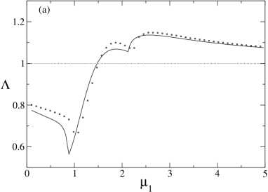
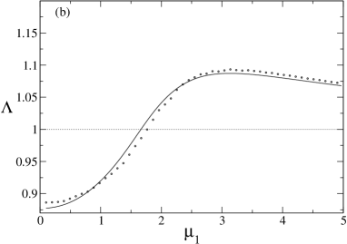
Figure 2: Floquet multipliers for a van der Pol oscillator array. Solid line represents analytical result, while dots represent results obtained from numerical calculations. The coupling parameters are $\kappa=1$, $\epsilon=0.1$, and (a) $\mu_{2}=0.8$, (b) $\mu_{2}=1.5$.

The synchronization condition for the array of globally coupled oscillators is obtained from (36-4) by setting $\lambda_{i}<1$ for all $i>1$, and can be expressed in terms of control parameters $\mu_{1}$ and $\mu_{2}$. In general, our method allows us to do a single calculation for a certain network configuration, and then obtain results for a variety of different oscillators in a straightforward fashion. To find the synchronization condition for a specific oscillator type it suffices to find the function $\phi^{\mathsf{R}}$ which characterizes the resonant terms in the equation of motion of the uncoupled oscillator. We illustrate this in several examples and compare our approximating solutions with numerical results. Agreement between analytical and numerical calculation is good even when using only first order corrections in $\epsilon$. We retrieve result from [15] as a special case of our general result.

5.1 Van der Pol oscillator arrays

Consider a network of globally coupled van der Pol oscillators described in Sec. 2.1. From (14) we find that the resonant terms are described by $\phi^{\mathsf{R}}=1/2-w\bar{w}/8$, and hence $R(r)=1/2-r^{2}/8$, $\Theta(r)=0$. From (34) we find that the inphase state exists for $r=2\sqrt{1+\kappa\cos\delta/Z}$. By substituting expressions for $R(r)$ and $\Theta(r)$ in (36) and (4) we find the Floquet exponents for the synchronous solution

$$\lambda_{2} = -\frac{\epsilon}{2}\left(1+\frac{\kappa}{Z}\cos\delta\right)$$ (40)

$$\lambda_{n,n+1} = -\frac{\epsilon}{2}\left(1+2\frac{\kappa}{Z}\cos\delta\right)\pm\frac{\epsilon}{2}\sqrt{\left(1+\frac{\kappa}{Z}\cos\delta\right)^{2}-\left(\frac{\kappa}{Z}\sin\delta\right)^{2}}.$$ (41)

In order to test our results we evaluate Floquet multipliers numerically and compare them to the values estimated from (41). The results are $\mathcal{O}(\epsilon)$ close (Fig. 2).

5.2 Van der Pol–Duffing equation

  

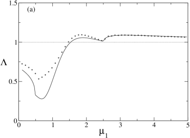
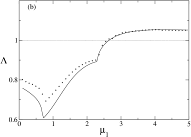
Figure 3: Floquet multipliers for a van der Pol-Duffing array. Coupling parameters are $\alpha=-0.2$, $\kappa=1$, $\epsilon=0.1$, and (a) $\mu_{2}=0.8$, (b) $\mu_{2}=1.5$.

In a recent study of micromechanical and nanomechanical resonators models using parametrically driven Duffing oscillators [25] and van der Pol–Duffing oscillators [4] are proposed. The van der Pol–Duffing equation

$$x^{\prime\prime}+x-\epsilon(1-x^{2})x^{\prime}-\epsilon\alpha x^{3}=0,$$ (42)

is obtained from the van der Pol equation by an addition of a cubic term. By switching to complex coordinates (11) and writing (42) in normal form we obtain

$$z^{\prime} = -iz+\frac{\epsilon}{8}(4z-z^{2}\bar{z}+i3\alpha z^{2}\bar{z})$$

$$\bar{z}^{\prime} = i\bar{z}-\frac{\epsilon}{8}(-4\bar{z}+z\bar{z}^{2}+i3\alpha z\bar{z}^{2}).$$

The resonant part of the nonlinearity is given by $\phi^{\mathsf{R}}(r)=(4-r^{2}+i3\alpha r^{2})/8$. The real part of $\phi^{\mathsf{R}}$ is the same as in the case of van der Pol oscillator, so this system has the same inphase solution. Substitute the real part $R(r)=1/2-r^{2}/8$ and imaginary part $\Theta(r)=3\alpha r^{2}/8$ of $\phi^{\mathsf{R}}$ in (36) and (4) to find the approximate Floquet exponents

$$\lambda_{2} = -\frac{\epsilon}{2}\left(1+\frac{\kappa}{Z}\cos\delta\right)$$ (43)

$$\lambda_{n,n+1} = -\frac{\epsilon}{2}\left(1+2\frac{\kappa}{Z}\cos\delta\right)$$

$$\pm\frac{\epsilon}{2}\sqrt{\left(1+\frac{\kappa}{Z}\cos\delta\right)^{2}-\left(\frac{\kappa}{Z}\sin\delta\right)^{2}+3\alpha\frac{\kappa}{Z}(2\sin\delta+\frac{\kappa}{Z}\sin 2\delta)}.$$

The numerical simulations (Fig. 3) support our result. Note that it follows from (20) that our approximations can be expected to break down for small values of $\mu_{1}$.

5.3 Synchronizing sources and sinks

Figure 4: The radius of the periodic, inphase solution is obtained by solving (34). For an array of elements (45) it is given by the intersection of the curve $rR(r)=r/2(r^{2}-3.6r+3.32)$ and the line $-\kappa\cos\delta/(2Z)r$. If the slope of the line is too small only the trivial solution $r=0$ exists, and the system does not exhibit limit cycle oscillations.

  

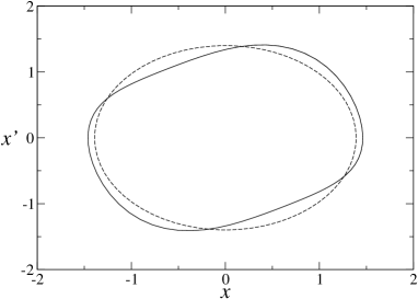
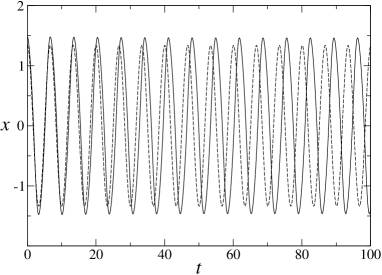
Figure 5: Phaseplane (left) and time diagram (right) of inphase limit cycle solution for coupled sources (45). Dashed line represents the solution for the truncated normal form system, and solid line numerical solution for the full system.

As noted in Remark 4, it is possible to turn a network of systems with flows that have only a source (or sink) at the origin into a network of synchronous limit cycle oscillators with an appropriate coupling. Consider a dynamical system described by

$$x^{\prime\prime}+x-\epsilon x^{\prime}\left[4x^{2}\left(1-\frac{3.6}{\sqrt{x^{2}+{x^{\prime}}^{2}}}\right)+3.32\right]=0.$$ (45)

Each individual system has only an unstable fixed point at the origin, and no other repellers or attractors. Coupling these systems as in (15-16), and switching to complex variables (11), gives the following equations of motion

$$z^{\prime} = -iz+i\epsilon f(z,\bar{z})$$ (46)

$$\bar{z}^{\prime} = i\bar{z}-i\epsilon f(z,\bar{z})$$ (47)

where the nonlinear term is

$$f(z,\bar{z})=\frac{z-\bar{z}}{2i}\left[\left(z+\bar{z}\right)^{2}\left(1-\frac{3.6}{\sqrt{z\bar{z}}}\right)+3.32\right].$$ (48)

If we keep resonant terms only, (46) and (47) become

$$z^{\prime} = -iz+\epsilon z\phi^{\mathsf{R}}(z\bar{z})$$ (49)

$$\bar{z}^{\prime} = i\bar{z}+\epsilon\bar{z}\phi^{\mathsf{R}}(z\bar{z})$$ (50)

with $\phi^{\mathsf{R}}=R(r)=1/2(z\bar{z}-3.6\sqrt{z\bar{z}}+3.32)$.

From (34) we find that the limit cycle solution does not exist for $-\kappa\cos\delta/(2Z)<0.08$. Below that value the coupled elements behave as unstable foci, which can be easily checked numerically. As $-\kappa\cos\delta/(2Z)$ increases above $0.08$ the system undergoes a supercritical saddle-node bifurcation of limit cycles, in which a stable and an unstable inphase limit cycle are created. These two solutions are are represented as the intersection of the curve $R=r/2(r^{2}-3.6r+3.32)$ and the line $R=-\kappa\cos\delta/(2Z)r$ in Fig. 4. For a suitable choice of coupling parameters it is possible to obtain inphase limit cycle solutions for the array of sources. In Fig. 5 we show oscillations of an element in the array, when the coupling parameters are set to $\kappa=1$, $\mu_{1}=1.2$ and $\mu_{2}=0.8$. The Floquet exponents for both limit cycles are readily obtained from (4). These results agree with numerical calculations to the expected error. In Fig. 6 we present results for the “stable” cycle.

  

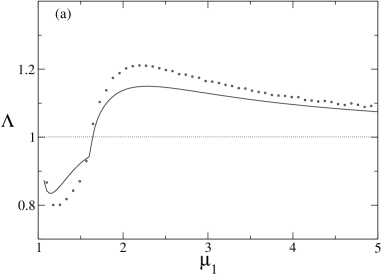
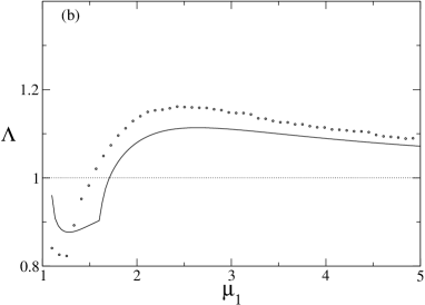
Figure 6: Floquet multipliers for coupled sources. $\kappa=1$, $\epsilon=0.1$, and (a) $\mu_{2}=0.8$, (b) $\mu_{2}=1.1$.

We note that a direct extension of the method discussed in the previous sections was used to derive these results, since the nonlinear term in (45) is not a polynomial (see [22]).

6 Conclusion

In our study of synchrony in globally coupled oscillator arrays we introduce a normal form based method, which has a number of advantages over methods commonly found in the physics literature. The method provides a clear and mathematically rigorous way of finding the onset of synchronization in the array with respect to changes in the control parameters. It allows for an easy distinction between contributions to the dynamics coming from the network configuration and those coming from the internal structure of the network elements. As a consequence, we are able to carry out calculations for particular network architectures without having to specify the exact form of the nonlinearities in the individual elements.

To apply these results to specific weakly nonlinear oscillators it is only necessary to find the function $\phi^{\mathsf{R}}$, which characterizes the resonant part of the nonlinearity, and substitute it in the general solution thus obtained. The function $\phi^{\mathsf{R}}$ does not depend on the coupling scheme, and is easily derived from the equations for the uncoupled systems. It is therefore tempting to think of synchronization classes as different systems may lead to the same $\phi^{\mathsf{R}}$.

Although we have chosen a very specific linear coupling in our exposition, the method can be applied to a variety of network configurations simply by retracing the steps we outlined. A similar calculation can be carried out even if there is a weak nonlinearity in the coupling equation (16) itself. Moreover, the method can be extended to higher orders in the small parameter in a straightforward fashion, and the procedure can be automated.

The analysis of the synchronous solution of the network (15-16) was particularly simple due its $S_{N}$ symmetry. When the network has less symmetry, or only local symmetries (see [26]), a similar reduction can be performed. In such networks one expects polysynchronous solutions, in which groups of oscillators within the network oscillate synchronously. One can further expect to obtain a pair of equations for each cluster of oscillators in the network [12]. The stability of these clusters can then be analyzed in a manner similar to the one introduced in this paper.

Although we have not treated the case of Josephson junctions, a similar analysis can also be performed. In fact we believe that coherent behavior in networks of various dynamical systems can be studied using the method of normal forms, and intend to investigate this in the future.

References

References

- [1] P. Tass. Phase Resetting in Medicine and Biology: Stochastic Modelling and Data Analysis. Springer-Verlag, New York, 1999.
- [2] S. Strogatz. Sync: The emerging science of spontaneous order. Athena, New York, 2003.
- [3] A. Pikovsky, M. Rosenblum, and J. Kurths. Synchronization – A universal concept in nonlinear sciences. Mathematics and its Applications. Cambridge University Press, Cambridge UK, 2001.
- [4] M. C. Cross, A. Zumdieck, R. Lifshitz, and J. L. Rogers. Synchronization by nonlinear frequency pulling. Phys. Rev. Lett., 2004. submited.
- [5] T. Heath. Beam steering of nonlinear oscillator arrays through manipulation of coupling phases. IEEE Trans. Antennas and Propagat., 52(7):1833–1842, 2004.
- [6] A.H. Nayfeh. Method of normal forms. Wiley Series in Nonlinear Science. John Wiley & Sons Inc., New York, 1993. A Wiley-Interscience Publication.
- [7] P. B. Kahn and Y. Zarmi. Nonlinear dynamics. Wiley Series in Nonlinear Science. John Wiley & Sons Inc., New York, 1998. Exploration through normal forms, A Wiley-Interscience Publication.
- [8] R.E.L. DeVille, A. Harkin, K. Josić, and T. Kaper. Applications of normal form theory to weakly nonlinear ordinary differential equations. SIAM J. Appl. Dyn. Syst., September 2004. submitted.
- [9] J.A. Murdock. Normal forms and unfoldings for local dynamical systems. Springer Monographs in Mathematics. Springer-Verlag, New York, 2003.
- [10] J. Carr. Applications of centre manifold theory, volume 35 of Applied Mathematical Sciences. Springer-Verlag, New York, 1981.
- [11] N. Kopell and G. B. Ermentrout. Symmetry and phaselocking in chains of weakly coupled oscillators. Comm. Pure Appl. Math., 39(5):623–660, 1986.
- [12] P. Ashwin and J. W. Swift. The dynamics of weakly coupled identical oscillators. J. Nonlinear Sci., 2(1):69–108, 1992.
- [13] F. C. Hoppensteadt and E. M. Izhikevich. Weakly connected neural networks. Springer-Verlag, New York, 1997.
- [14] S. Han, B. Bi, W. Zhang, and J. E. Lukens. Demonstration of Josephson effect submillimeter wave sources with increased power. Appl. Phys. Lett., 64(11):1424–1426, 1994.
- [15] S. Peleš and K. Wiesenfeld. Synchronization law for a Van der Pol array. Phys. Rev. E, 68(2):026220, 2003.
- [16] K. Wiesenfeld, P. Colet, and S. H. Strogatz. Synchronization transitions in a disordered Josephson series array. Phys. Rev. E, 76(3):404–407, 1996.
- [17] K. Wiesenfeld and J. W. Swift. Averaged equations for Josephson junction series arrays. Phys. Rev. E, 51(2):1020–1025, 1995.
- [18] A. A. Chernikov and G. Schmidt. Conditions for synchronization in Josephson-junction arrays. Phys. Rev. E, 52(4):3415–3419, 1995.
- [19] M. Dhamala and K. Wiesenfeld. Generalized stability law for Josephson series arrays. Phys. Lett. A, 292:269–274, 2002.
- [20] M. Ziane. On a certain renormalization group method. J. Math. Phys., 41(5):3290–3299, 2000.
- [21] J. K. Hale. Ordinary differential equations. Robert E. Krieger Publishing Co. Inc., Huntington, N.Y., second edition, 1980.
- [22] Yu. A. Mitropolsky and A. K. Lopatin. Nonlinear mechanics, groups and symmetry, volume 319 of Mathematics and its Applications. Kluwer Academic Publishers Group, Dordrecht, 1995. Translated from the 1988 Russian original by O. S. Limarchenko, A. N. Khruzin and T. P. Boichuk and revised by the authors.
- [23] S. M. Cox and A. J. Roberts. Initial conditions for models of dynamical systems. Phys. D, 85(1-2):126–141, 1995.
- [24] G. Haller. Chaos near resonance, volume 138 of Applied Mathematical Sciences. Springer-Verlag, New York, 1999.
- [25] R. Lifshitz and M. C. Cross. Response of parametrically driven nonlinear coupled oscillators with application to micromechanical and nanomechanical resonator arrays. Phys. Rev. B, 67:134302, 2003.
- [26] I. Stewart, M. Golubitsky, and M. Pivato. Symmetry groupoids and patterns of synchrony in coupled cell networks. to appear in SIAM J. Appl. Dynam. Sys.