Aggregation of finite size particles with variable mobility

Abstract

New model equations are derived for dynamics of self-aggregation of finite-size particles. Differences from standard Debye-Hückel DeHu1923 and Keller-Segel KeSe1970 models are: the mobility of particles depends on the configuration of their neighbors and linear diffusion acts on locally-averaged particle density. The evolution of collapsed states in these models reduces exactly to finite-dimensional dynamics of interacting particle clumps. Simulations show these collapsed (clumped) states emerge from smooth initial conditions, even in one spatial dimension.

Keywords: gradient flows, blow-up, chemotaxis, parabolic-elliptic system, singular solutions

Modeling finite size effects in the aggregation of interacting particles requires modifications of the class of Debye-Hückel equations. This problem is motivated by recent experiments using self-assembly of nano-particles in the construction of nano-scale devices XB2004 . Fundamental principles underlying the self-assembly at nano-scales are non-local particle interaction and nonlinear motion due to variations of mobility at these scales. The model should account for the change of mobility due to the finite size of particles and the nonlocal interaction among the particles. The local density (concentration) of particles is denoted by $\rho$. For particles interacting pairwise via the potential $-G(|\mathbf{r}|)$, the total potential at a point ${\mathbf{r}}$ is $\Phi({\mathbf{r}})=-\int\rho({\mathbf{r}}^{\prime})G(|{\mathbf{r}}-{\mathbf{r}}^{\prime})\mbox{d}{\mathbf{r}}^{\prime}=G*\rho$ where $*$ denotes convolution and $G>0$ for attracting particles. The velocity of the particle is assumed to be proportional to the gradient of the potential times the mobility of a particle, $\mu$. The mobility can be computed explicitly for a single particle moving in an infinite fluid. However, when several particles are present, especially in highly dense states, the mobility of a particle may be hampered by interactions with its neighbors. These considerations are confirmed, for example, by the observation that the viscosity of a dense suspension of hard spheres in water diverges, when the density of spheres tends to its maximum value. Many authors have tried to incorporate the dependence of mobility on local density by putting $\mu=\mu(\rho)$ and assuming $\mu(\rho)\to 0$ as $\rho\to\rho_{\hbox{\small max}}=1$ Velazquez2002 . Vanishing mobility leads to the appearance of weak solutions in the equations, to singularities and, in general, to massive complications and difficulties in both theoretical analysis and computational simulations of the equations.

Alternatively, we suggest that the mobility $\mu$ should depend on an averaged density $\overline{\rho}$ over some sampling volume, rather than on either the potential, or the exact value of the density at a point. This assumption makes sense from the viewpoints of both physics and mathematics. From the physical point of view, the mobility of a finite-size particle must depend on the configuration of particles in its vicinity. While attempts have been made to approximate this dependence by using derivatives of the local density, this approach may lead to unphysical negative diffusivity Villain1991 . Hence, we assume instead that the local mobility depends on an integral quantity $\overline{\rho}$ which is computed from the density as $\overline{\rho}=H*\rho$. Here $H({\mathbf{r}})$ is a local filter function, which may be of much shorter range than the potential $G$. Several filter functions are possible, with examples $H({\mathbf{r}})$ being a $\delta$-function, an exponential (or inverse-Helmholtz in 1D) or a top-hat filter. Alternatively, for crystal growth applications, one may assume a filter function $H({\mathbf{r}})$ with zero average, so the mobility does not depend on the magnitude of the density, only on the relative position of particles. The mathematical analysis and the reduction property derived in this paper holds, regardless of the shape of the filter function $H$ and the potential $G$ is, so long as they are both nice (e.g., piecewise smooth) functions.

Aim of the paper This paper treats the following continuity equation for the evolution of density,

$$\frac{\partial\rho}{\partial t}=-\,{\rm div}\,{\mathbf{J}}\quad\hbox{with}\quad{\mathbf{J}}=-\,D\nabla\overline{\rho}-\,\mu(\overline{\rho})\rho\nabla\Phi\,.$$ (1)

Here $D\geq 0$ is a constant, while $\overline{\rho}$ and $\Phi$ are defined by two convolutions involving, respectively, the filter function $H$ and the potential $G$,

$$\overline{\rho}=H*\rho\quad\hbox{and}\quad\Phi=G*\rho\,.$$ (2)

While model (1,2) preserves the sign of $\rho$, we shall see that it allows the formation of $\delta$-function singularities even when $D>0$ and in the case of one dimension. The generality and predictive power of model (1,2) can be demonstrated by enumerating a few of its subcases. For example, when $H({\mathbf{r}})=\delta({\mathbf{r}})$ and $G(x)=e^{-|{\mathbf{r}}|/l}$ this system reduces to the generalized chemotaxis equation Velazquez2002 . For the choice $G=\delta^{\prime}({\mathbf{r}})$, $H=\delta^{\prime}({\mathbf{r}})$ one obtains a variant of the inviscid Villain model for MBE evolution Villain1991 . If the range of $G$ (denoted by $l$) is sufficiently small, one may approximate (at least formally) the integral operator in $\Phi=G*\rho$ as a differential operator acting on the density $\rho$, namely, $\Phi=\rho+l\nabla\cdot(l\nabla\rho)$. As was demonstrated in MPXB2004 , equation (1) then becomes a generalization of the viscous Cahn-Hilliard equation, describing aggregation of domains of different alloys. In the case that $\mu$ is constant, $H(x-y)=\delta(x-y)\,,$ and $G$ is the Poisson kernel, then equation (1) becomes the Poisson-Smoluchowski equation for the interaction of gravitationally attracting particles under Brownian motion Ch1939 .

All four subcases of model (1,2) described above require a singular choice of the smoothing kernels $G$ and $H$. However, the generalized functions required in these singular choices may be approximated with arbitrary accuracy by using sequences of nice (for example, piecewise smooth) functions. We shall concentrate on cases where the functions $H$ and $G$ remain nice, and derive the results in this more general, more regular, setting. Thus, regularization introduces additional generality, which enables analytical progress and makes numerical solution of the equations easier.

Gradient flow motivation Model (1,2) may also be motivated from the viewpoint of gradient flows and thermodynamics. The associated free energy decreases monotonically in time and remains finite even when the solutions tend to a set of delta-functions. This energy remains finite for all choices of $\mu(\overline{\rho})$. In contrast, the traditional approach in which the mobility is assumed to depend on the un-smoothed density $\mu(\rho)$ will fail by allowing the energy to become infinite. This additional energetic argument reinforces the choice of the regularized model in (1,2). The calculation will be performed in arbitrary spatial dimensions. For the energy to be well-defined, we assume that the function $G$, describing the interaction between two particles, is everywhere positive, so the interaction is always attractive. In one dimension, we also assume that the kernel function $G$ is symmetric and in $n$ dimensions that the interaction is central. These assumptions are physically viable for all the previous subcases. Our derivation for the free energy will remain valid for an arbitrary filter function $H$.

We start with equation (1) for mass conservation, in the case when the mobility $\mu(\overline{\rho})$ in the particle flux $\mathbf{J}$ is not constant. We shall derive a variant of equation (1) as a gradient flow defined by,

$$\frac{\partial\rho}{\partial t}=-\,{\rm grad}E\big{|}_{\rho}\,,\hbox{ or }\Big{\langle}\frac{\partial\rho}{\partial t}\,,\,\Psi\Big{\rangle}=-\,\Big{\langle}\frac{\delta E}{\delta\rho}\,,\,\Psi\Big{\rangle}\,,$$ (3)

where $\langle f\,,\,\Psi\rangle=\int f\Psi\,d^{n}x$ is the $L^{2}$ pairing, for a suitable test function $\Psi$ and where $E$ is the following energy,

$$E[\rho]=D\!\!\int\!\!\overline{\rho}(\log\overline{\rho}-1)\mbox{d}x+\frac{1}{2}\!\!\int\!\!\rho\,\Phi\,\mbox{d}x\,,$$ (4)

with $\Phi=G*\rho$ and $\overline{\rho}=H*\rho$. The first term in energy $E[\rho]$ in (4) decreases monotonically in time for linear diffusion of $\overline{\rho}$. The second term defines the $H^{-1}$ norm of $\rho$ in 1D for the choice $G(x)=\exp(-|x|/\alpha)$, and it provides a generalization of this norm for an arbitrary (but positive and symmetric) function $G$. Energy $E[\rho]$ in (4) remains finite, even when the solution for the density $\rho$ concentrates into a set of $\delta$-functions.

The variation of the free energy $E[\rho]$ in equation (4) is

$$\delta E[\rho]=\int(DH*(\log\overline{\rho})+\Phi)\,\delta\rho\,d\,^{n}x\,,$$

where the density variation $\delta\rho$ is chosen in the form,

$$\delta\rho=-\rm{div}\big{(}\rho\mu(\overline{\rho})\nabla{\Psi}\big{)}\,,$$

determined by the function $\Psi$, which is assumed to be smooth, footnote . After integrating by parts, the corresponding variational derivative is

$$\Big{\langle}\frac{\delta E}{\delta\rho}\,,\,\Psi\Big{\rangle} = -\Big{\langle}\rm{div}\Big{(}\rho\mu(\overline{\rho})\nabla\big{(}(DH*(\log\overline{\rho})+\Phi)\big{)}\Big{)}\,,\,\Psi\Big{\rangle}\,.$$

The resulting variant of equation (1) is, cf. (3)

$$\frac{\partial\rho}{\partial t}=-\,{\rm div}\,{\mathbf{J}}_{m}\,,\quad{\mathbf{J}}_{m}=-\,\rho\mu(\overline{\rho})\big{(}DH*\frac{1}{\overline{\rho}}\nabla\overline{\rho}+\nabla\Phi\big{)}\,,$$ (5)

in which the linear diffusion of density $\overline{\rho}$ is mollified by smoothing with $H$. Finally obtaining the particle flux $\mathbf{J}$ in equation (1) requires simplifying the first term of ${\mathbf{J}}_{m}$ in (5) to $D\nabla\overline{\rho}$ . Thus, only the contribution $-\mu(\overline{\rho})\rho\nabla\Phi$ to the particle flux in equation (1) is variational.

Energetics The free energy $E[\rho]$ in (4) decreases monotonically in time under the evolution equation (5). A direct calculation yields,

$$\frac{dE[\rho]}{dt}=-\int\frac{1}{\rho\mu_{(}\overline{\rho})}\,|{\mathbf{J}}_{m}|^{2}\,d\,^{n}x\,.$$ (6)

We shall see that the resulting mass-conserving motion of finite-size particles governed by (5) leads to a type of ‘clumping’ of the density $\rho$ into a support set consisting of $\delta$-functions. One may check that this monotonic decrease of energy persists for more general functions, including these weak solutions supported on $\delta$-functions, as discussed below. These weak solutions are then found to spontaneously emerge in numerical simulations of equation (1) and dominate the initial value problem.

Dynamics of clumpons We consider motion under equations (1,2) in one spatial dimension. Substituting the following singular solution ansatz

$$\rho(x,t) = \sum_{i=1}^{N}w_{i}(t)\delta(x-q_{i}(t))\,,$$ (7)

into the one-dimensional version of either equation (1) or (5) with $D=0$ and integrating the result against a smooth test function $\phi$ yields a closed set of equations for the parameters $w_{i}(t)$ and $q_{i}(t)$, $i=1,2,\dots,N,$ of the solution ansatz (7). Namely,

$$\dot{w}_{i}(t)=0\,,\quad\dot{q}_{i}(t)=-\sum_{j=1}^{N}w_{j}\mu\big{(}\overline{\rho}\big{)}G\,^{\prime}(q_{i}-q_{j})\,,$$ (8)

where $\overline{\rho}=\sum_{m=1}^{N}w_{m}H(q_{j}(t)-q_{m}(t))$. Thus, the density weights $w_{i}(t)=w_{i}(0)=w_{i}$ are preserved for $i=1,2,\dots,N$, and the corresponding positions $q_{i}(t)$ follow the characteristics of the velocity ${\mathbf{u}}=-\mu(\overline{\rho})\nabla G*\rho$ along the Lagrangian trajectories defined by $x=q_{i}(t)$. This result holds in any number of dimensions, modulo changes to allow singular solutions supported along moving curves in 2D and moving surfaces in 3D. When $D\neq 0$ and div$D\nabla\overline{\rho}\simeq\rho$, the weights $w_{i}$ decay essentially exponentially in time, under evolution by equation (1).

In Fig. 1, we demonstrate that the solutions (8) do indeed appear spontaneously in a numerical simulation of equation (1) with $D=0.02$. Hence, they are essential in understanding its dynamics. The simulation started with a smooth (Gaussian) initial condition for density $\rho$. Almost immediately, one observes the formation of several singular clumpons, which evolve to collapse eventually into a single clumpon. Observe that the mass of each individual clumpon remains almost exactly constant in the simulations, as required by equation (8) with $D=0$. Also note that the masses of two individual clumpons add up when they collide and “clump” together. Consequently, all the mass eventually becomes concentrated into a single clumpon, whose mass (amplitude) is the total mass of the initial condition. This simulation shows that for a general system (1) the long-term evolution evolves into the collective motion of a finite number of individual clumpons. This conclusion is supported by analysis showing the superposition of clumpons represented by the singular solution (7) is an invariant manifold of the gradient flow equations (1).

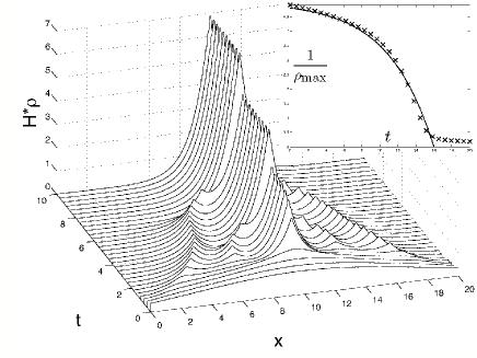
Figure 1: Numerical simulation demonstrates the emergence of particle clumps, showing formation of density peaks in a simulation of the initial value problem for equation (1) using smooth initial conditions for density with $l=1$, $G(x)=H(x)=\exp(-|x|)$, $\mu(\overline{\rho})=1$. The vertical coordinate represents $\overline{\rho}=H*\rho$, which remains finite even when the density forms $\delta$-functions. Insert: The behavior of the inverse amplitude of the maximum peak $1/\rho_{m}(t)$ (crosses) versus analytical solution of equation (9) (solid line).

Rate of blow up Analysis of the evolution of a density maximum reveals the clumping process results from the nonlinear instability of the gradient flow in equation (1) when $D=0$. For a particular case $G=e^{-|x|/\alpha}$, one may show that for large enough peak, a density maximum $\rho_{m}(t)=\rho(x_{m}(t),t)$ becomes infinite in finite time. The motion of the maximum is governed by

$$\frac{d}{dt}\rho_{m}=\frac{1}{\alpha^{2}}\left(\rho_{m}^{2}-\rho_{m}\Phi(x_{m})\right)\geq\frac{1}{\alpha^{2}}\left(\rho_{m}^{2}-\rho_{m}M\right),$$ (9)

where $M=\int\rho\mbox{d}x$ is total mass and we have used the fact that $\Phi$ satisfies $\Phi-\alpha^{2}\Phi_{xx}=\rho$. The last inequality holds, because $G\leq 1$ is bounded and $\rho$ is everywhere positive. Thus, if at any point the maximum of $\rho$ exceeds the (scaled) value of the total mass, then the value of the density maximum $\rho_{m}(t)$ must diverge in finite time, which produces $\delta$-functions in finite time. From (9), the density amplitude must diverge as $\rho_{m}\simeq\alpha^{2}/(t_{0}-t)$. To illustrate this divergence, we have plotted the comparison between the predicted collapse of $1/\rho_{m}$ and numerics in the insert of Fig. 1. The formation of singularities in Fig. 1 occurs both at the maximum, and elsewhere, The subsidiary peaks eventually collapse with the main peak.

Competing length scales of $H$ & $G$ An interesting limiting case arises, when the scale of non-locality of $H$ is much shorter than the range of the potential $G$. Formally, this limit corresponds to $H(x)\rightarrow\delta(x)$. In practice, we may select a sequence of piecewise smooth functions $H_{\epsilon}(x)=\exp(-|x|/\epsilon)/(2\epsilon)$ which converge weakly to a $\delta$-function. For each function $H_{\epsilon}(x)$ in this sequence, no matter how small (but positive) the value of $\epsilon$, the exact ODE reduction (8) still holds. What happens in the limit of very small epsilon, as $\epsilon\to 0$? In investigating the limit as $\epsilon\to 0$, we performed a sequence of numerical simulations with the function $G(x)=\exp(-|x|/\alpha)$ being held fixed and $H_{\epsilon}(x)=\exp(-x/\epsilon)/(2\epsilon)$ varying, for a sequence of decreasing values of the ratio $\epsilon/\alpha$. This simulation is illustrated in Fig. 2 for $\epsilon/\alpha=1/10$, which demonstrates the formation of flat clumps of solutions. The mechanism of this phenomenon is the following. The vanishing mobility at $\overline{\rho}=1$ caps the maximal density at $\overline{\rho}=1$ in the long-term. This leads to the appearance of flat mesas in $\overline{\rho}(x)$ for large $t$. On the other hand, when $H(x)\rightarrow\delta(x)$, $\overline{\rho}(x,t)\rightarrow\rho(x,t)$ pointwise in $x$, which forces $\rho(x,t)$ to develop a flat mesa, or plateau, structure in which the maximum is very close to unity, as well. This is precisely what is predicted for the chemotaxis equation with $H(x)=\delta(x)$ and $\mu(\rho)=1-\rho$ Velazquez2002 .

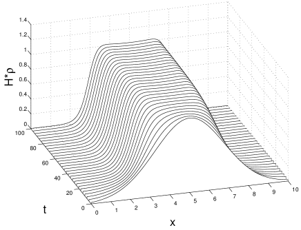
Figure 2: Evolution of a Gaussian initial condition for $\rho$(x,0) with $\mu(\overline{\rho})=1-\overline{\rho}$ and $H=\exp(-|x|/\epsilon)/(2\epsilon)$ where $\epsilon=\alpha/10$. The solution quickly forms a plateau of maximal possible density ($\rho_{\hbox{\small max}}=1$).

In the limit $H\rightarrow\delta$, model (1,2) recovers ordinary diffusion of local density. This is a singular limit, because it increases the order of the differentiation in the equation. Since ordinary diffusion is known to prevent collapse in one dimension Ho2003 , this singular limit should be of considerable interest for further analysis.

Conclusion and Open Problems A new model was proposed and analyzed for the collective aggregation of finite-size particles driven by the force of mutual attraction. Starting from smooth initial conditons, the solution for the particle density in this model was found to collapse into a set of delta-functions (clumps), and the evolution equations for the dynamics of these clumps was computed analytically. The energy derived for this model is well defined even when density is supported on $\delta$-functions. The mechanism for the formation of these $\delta$-function clumps is the nonlinear instability governed by the Ricatti equation (9), which causes the magnitude of any density maximum to grow without bound in finite time. At first sight, it may seem that the emergence of $\delta$-function peaks in the solution might be undesirable and perhaps should be avoided. However, these $\delta$-functions may be understood as clumps of matter, and the model guarantees that any solution eventually ends up as a set of these clumps. Consequently, further collective motion of these clumps may be predicted using a (rather small-dimensional) system of ODEs, rather than dealing with the full non-local PDEs. The question of how many clumps arise from a given initial condition remains to be considered. One may conjecture that clump formation is extensive; so that each clump forms from the material within the range of the potential $\Phi$, determined by $G$. On a longer time scale, the clumps themselves continue to aggregate, as determined by the collective dynamics (8) of weak solutions (7). This clump dynamics is also a gradient flow; so that eventually only one clump remains.

An analogy to point vortex solutions of Euler’s equations for two-dimensional ideal hydrodynamics may be drawn here. Prediction of motion of inviscid fluid is governed by a set of nonlinear PDE in which pressure introduces non-locality. A drastic simplification of motion occurs, when all the vorticity is concentrated in delta-functions (point vortices) Saffman-book . The motion of point vortices lies on a singular invariant manifold: if started with a set of point vortices, the fluid structure will remain a set of point vortices. However, a smooth initial condition for vorticity does not split into point vortices under the Euler motion. In the present model, though, the physical attraction drives any initial conditions towards a set of delta-functions, so one is guaranteed to obtain effectively finite-dimensional behavior in the system after a rather short initial time.

Because two scales are present in the smoothing functions $H$ and $G$, the effects of boundary conditions warrant further study. For example, the $H\rightarrow\delta$ limit should also allow formation of boundary layers. Here, these boundary issues were avoided by using periodic boundary conditions. However, it is natural in physical situations to apply, e.g., Neumann boundary conditions to the particle flux $\mathbf{J}$. Thus, the issue of boundary conditions may become important in a more physically realistic setting.

Acknowledgments. We thank P. Constantin, B. J. Geurts, J. Krug and E. S. Titi for encouraging discussions and correspondence about this work. We are grateful for partial support by US DOE, under contract W-7405-ENG-36 for Los Alamos National Laboratory, and Office of Science ASCAR/AMS/MICS.

References

- (1) P. Debye and E. Hückel, Phys. Z. 24, 305 (1923).
- (2) E.F. Keller and L.A. Segel, J. Theo. Biol. 26, 399 (1970); Ibid. J. Theo. Biol. 30, 225 (1971).
- (3) D. Xia and S. Brueck, Nano Letters, 4, 1295(2004).
- (4) J.J.L. Velazquez, SIAM J. Appl. Math, 62, 1581 (2002).
- (5) J. Villain, J. Phys. France I 1, 19 (1991).
- (6) K. Mertens, V. Putkaradze, D. Xia and S. Brueck, Nano Letters, under consideration (2004).
- (7) S. Chandrasekhar, An introduction to the theory of stellar structure (Dover, 1939). Cites research by M. V. Smoluchowski, Z. Phys. Chem. 92, 129-168 (1917). USA. 95:9280-9283.
- (8) D. Horstmann, MPI Leipzig Report (2003).
- (9) D.D. Holm, J.E. Marsden and T.S. Ratiu, Adv. in Math., 137, 1-81 (1998). http://xxx.lanl.gov/abs/chao-dyn/9801015.
- (10) These gradient flow properties of the smooth solutions are also preserved for the weak solutions.
- (11) F. Otto, Comm. Partial Diff. Eqs. 26, 101-174 (2001).
- (12) P.G. Saffman, Vortex Dynamics. Cambridge Univ. Press (1992).