The large-scale structure of passive scalar turbulence

Abstract

We investigate the large-scale statistics of a passive scalar transported by a turbulent velocity field. At scales larger than the characteristic lengthscale of scalar injection, yet smaller than the correlation length of the velocity, the advected field displays persistent long-range correlations due to the underlying turbulent velocity. These induce significant deviations from equilibrium statistics for high-order scalar correlations, despite the absence of scalar flux.

Turbulent flows are systems far away from equilibrium, characterized by a flux of energy through a range of scales. This cascade process is often accompanied by strongly non-gaussian statistics and nontrivial scaling properties F95 . Passive scalar turbulence is no exception, in this respect. Its understanding has recently undergone remarkable progress, with results thoroughly reviewed in Ref. FGV01 . A passive scalar field $\theta({\bm{x}},t)$, like dilute dye concentration or temperature in appropriate conditions, transported by an incompressible velocity field ${\bm{v}}({\bm{x}},t)$, evolves according to

$$\partial_{t}\theta+{\bm{v}}\cdot{\bm{\nabla}}\theta=\kappa\Delta\theta+f\;,$$ (1)

where $f$ is a source of scalar fluctuations that acts at a lengthscale $L$. The velocity field is assumed to be turbulent and characterized by a self-similar statistics (e.g. $(v(x+r)-v(x))\sim r^{1/3}$ according to Kolmogorov’s 1941 theory) in the range of scales delimited above by the velocity correlation length $L_{v}$ and below by the viscous scale $\eta$. Passive scalar fluctuations generated at the scale $L$ form increasingly finer structures due to velocity advection and this process results in a net flux of scalar variance to small scales, where it is eventually smeared out by molecular diffusivity at a scale $r_{d}$. Here we will consider the case where these scales are ordered as follows: $L_{v}\gg L\gg\eta,r_{d}$. In the range $L\gg r\gg r_{d}$ the average scalar flux is constant and equals the average input rate: this is the well studied inertial-convective range where $\theta$ displays non-gaussian statistics and anomalous scaling SS00 ; W01 . Conversely, at scales larger than $L$ there is no scalar flux. Accordingly, one would expect Gaussian statistics and equipartition of scalar variance, i.e. the hallmarks of statistical equilibrium. This expectation is correct at $r\gg L_{v}$, where the dynamics of the large-scale passive scalar is ruled by an effective diffusion equation resulting in a Gaussian statistics. However, in the intermediate range $L_{v}\gtrsim r\gtrsim L$, deviations from “thermal equilibrium” might arise as a consequence of turbulent transport. Indeed, Falkovich and Fouxon FF04 have recently shown — in the context of the Kraichnan model of passive scalar advection where the velocity field is gaussian, self-similar and short-correlated in time K68 — that the scalar field shows a highly nontrivial behavior at scales larger than the pumping correlation length $L$, with significant differences from Gibbs statistical ensemble. In this Letter we show that these results extend to passive scalar advection by a realistic flow, namely two-dimensional Navier-Stokes turbulence in the inverse cascade range. This flow has been studied in great detail both experimentally (in fast flowing soap films KG02 and in shallow layers of electromagnetically driven electrolyte solutions T02 ) and numerically SY93 ; BCV00 . The velocity is statistically homogeneous and isotropic, scale-invariant with exponent $1/3$ (no intermittency corrections to Kolmogorov scaling) and with dynamical correlation times. This flow has also been utilized to investigate passive scalar transport in the scalar flux range $L\gtrsim r\gtrsim r_{d}$ CLMV00 ; CV01 and multi-particle dispersion, an intimately related subject BC00 ; CP02 . From this ensemble of studies it emerged that the lessons drawn from the study of the Kraichnan model are indeed relevant for the qualitative understanding of passive scalar transport by realistic flows; and this will turn out to be true for the present case as well.

Some basic, although incomplete, information about the scalar statistics in the supposed “thermal equilibrium range” can be gained by studying the isotropic spectrum $E(k)=2\pi k\langle|\hat{\theta}({\bm{k}})|^{2}\rangle$ for $kL\gtrsim 1$. Let us recall that the equilibrium statistics for the scalar field would be described by the Gibbs functional ${\cal P}[\hat{\theta}]=Z^{-1}\exp[-\beta\int|\hat{\theta}({\bm{k}})|^{2}d{\bm{k}}]$, i.e. the Fourier modes should behave as independent Gaussian variables with equal variance $1/(2\beta)$. As shown in Fig. 1, we observe $E(k)\sim k$, in agreement with equipartition arguments; moreover, the statistics of single Fourier modes is indistinguishable from Gaussian. However, we anticipate that from those findings alone one cannot state conclusively that large-scale passive scalar is in a thermal equilibrium state, given that they do not allow to rule out the possibility of long-range correlations for higher order observables (e.g. four-point scalar correlations).

A more refined description of the large-scale properties of passive scalar can be obtained in terms of the coarse-grained field

$$\theta_{r}({\bm{x}},t)=\int G_{r}({\bm{x}}-{\bm{y}})\theta({\bm{y}},t)\,d{\bm{y}}$$ (2)

where $G_{r}$ acts as a low-pass filter in Fourier space (for instance, the top-hat filter $G_{r}({\bm{x}}-{\bm{y}})=1/(\pi r^{2})$ if $|{\bm{x}}-{\bm{y}}|<r$ and zero otherwise; or the Gaussian filter $G_{r}({\bm{x}}-{\bm{y}})=(2\pi r^{2})\exp[-|{\bm{x}}-{\bm{y}}|^{2}/(2r^{2})]$). For $r\to 0$ the filter reduces to a two-dimensional $\delta$-function and therefore $\theta_{r}\to\theta$.

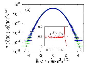
Figure 1: (a) Passive scalar and velocity spectra. The data result from the time integration of the two-dimensional Navier-Stokes equations $\partial_{t}{\bm{v}}+{\bm{v}}\cdot{\bm{\nabla}}{\bm{v}}=-{\bm{\nabla}}p+\nu\Delta{\bm{v}}+{\bm{F}}-\alpha{\bm{v}}$ and eq. (1) by a pseudospectral method on a 1024² grid. The passive scalar is injected by a Gaussian, $\delta$-correlated in time, statistically homogeneous and isotropic forcing restricted to a narrow band of wavenumbers. The initial condition for the velocity field is a configuration taken from a previous long-time integration and thus already at the statistically stationary state. The passive scalar starts from a zero field configuration, and after a transient of a few large-eddy turnover times $\tau_{v}=L_{v}/v_{rms}$ where $L_{v}$ is the integral scale of the velocity field, it reaches its own statistically steady state as well. Time averages are taken after this relaxation time has elapsed, for a total duration of more than $10^{4}$ scalar correlation times $\tau_{L}\approx\tau_{v}(L/L_{v})^{2/3}$. Here $L/L_{v}\approx 0.02$. The velocity spectrum agrees with the Kolmogorov prediction $k^{-5/3}$ and the passive scalar one follows very closely the equipartition spectrum in two-dimensions $E(k)\sim k$ (see also the inset of panel (b)). (b) The marginal probability density function of a single Fourier amplitude $\hat{\theta}({\bm{k}})$ is indistinguishable from a Gaussian (dotted curve) for all wavenumbers in the range $L^{-1}\gtrsim k\gtrsim L_{v}^{-1}$. Here are shown three wavenumbers with $kL=0.5,0.25,0.12$. In the inset is shown the spectral density $\langle|\hat{\theta}({\bm{k}})|^{2}\rangle$ that shows a neat plateau at $kL\ll 1$ (notice the linear scale on the vertical axis).

The statistics of $\theta$ is typically supergaussian JW91 ; JPG91 : its probability density function has exponential-like tails even for a gaussian driving force $f$. Indeed, in the latter case it can be shown that $\theta$ is the product of two independent random variables $\theta\stackrel{{\scriptstyle\Delta}}{{=}}\phi\sqrt{F_{0}T}$ where $\phi$ is a gaussian variable of zero mean and unit variance, $F_{0}$ is the average injection rate of scalar fluctuations, and $T$ is a positive-defined random variable, independent from $\phi$. The variable $T$ is essentially the time taken by a spherical blob of minute initial size to disperse across a length $L$ for a given flow configuration FMNV99 ; CV03 . For example, assuming a poissonian distribution for the rare events when $T$ exceeds its average value yields exponential tails for the pdf of $\theta$ SS94 . The distribution of $\theta_{r}$ is supergaussian as well; however, as $r$ increases above the forcing correlation length, the probability density of $\theta_{r}$ tends to a gaussian distribution, as it is clearly seen by the scale-dependence of the distribution flatness and hyperflatness (see Fig. 2).

Within the framework of Gibbs statistical equilibrium, the scalar field has vanishingly small correlations above the scale $L$: therefore one could view $\theta_{r}$ as the sum of $N\approx(r/L)^{2}$ independent random variables (identically distributed as $\theta$) divided by $N$. By central limit theorem arguments remark , the moments of order $2n$ of the coarse-grained scalar field (odd-order moments vanish by symmetry) should then scale as $N^{-n}$, giving $\langle(\theta_{r})^{2n}\rangle\sim\langle\theta^{2}\rangle^{n}(r/L)^{-2n}$. This is a very good estimate for $n=1$: indeed, as shown in Fig. 3, the product $(r/L)^{2}\langle\theta_{r}^{2}\rangle$ has a very neat plateau. This is consistent with the fast decay of the two-point scalar correlation $\langle\theta({\bm{x}},t)\theta({\bm{x}}+{\bm{r}},t)\rangle$ at $r\gtrsim L$. Indeed, in this case the second-order moment $\langle\theta_{r}^{2}\rangle=\int d{\bm{y}}_{1}d{\bm{y}}_{2}G_{r}({\bm{y}}_{1}-{\bm{x}})G_{r}({\bm{y}}_{2}-{\bm{x}})\langle\theta({\bm{y}}_{1},t)\theta({\bm{y}}_{2},t)\rangle$ is dominated by contributions with $|{\bm{y}}_{1}-{\bm{y}}_{2}|\lesssim L$ yielding $\langle\theta_{r}^{2}\rangle\sim\langle\theta^{2}\rangle(r/L)^{-2}$. Alternatively, by Fourier transforming the coarse-grained field one obtains $\langle\theta_{r}^{2}\rangle=\int|\hat{G}_{r}({\bm{k}})|^{2}\langle|\hat{\theta}({\bm{k}},t)|^{2}\rangle d{\bm{k}}\simeq\langle\theta^{2}\rangle(r/L)^{-2}$, since the transformed filter $\hat{G}_{r}({\bm{k}})$ is close to unity for $kr\ll 1$ and falls off very rapidly for $kr\gtrsim 1$, and $|\hat{\theta}({\bm{k}},t)|^{2}\simeq\langle\theta^{2}\rangle/(\pi L^{2})$. In summary, two-point statistics appears to be consistent with Gibbs equilibrium ensemble. The situation for multi-point correlations will turn out to be different.

A careful inspection of higher-order moments shows a less good agreement with central-limit theorem estimates (see Fig. 3): this points to the existence of subleading contributions to the moments $\langle\theta_{r}^{2n}\rangle$ for $n>1$ arising from long-range correlations of multiple scalar products. In order to quantify more precisely the rate of convergence to gaussianity and its relationship to long-range correlations, it is useful to consider the cumulants of the random variable $\theta_{r}$. According to central limit theorem remark , the cumulant of order $2n$ should vanish with $N^{-2n+1}$ leading to an expected scaling $\langle\langle\theta_{r}^{2n}\rangle\rangle\sim\langle\langle\theta^{2n}\rangle\rangle(r/L)^{-4n+2}$. Let us reiterate that the former expression is expected to be valid in absence of scalar correlations across lengthscales $r\gtrsim L$.

Figure 2: The flatness and hyperflatness of the coarse-grained scalar field as a function of $r/L$, normalized by their gaussian values $(2n-1)!!$. For $r\to 0$ the curves tend to the flatness factors of the field $\theta$: the numerical values correspond to a supergaussian probability density function $\ln p(\theta)\sim-\theta^{1.6}$.

For $n=1$ we have $\langle\langle\theta_{r}^{2}\rangle\rangle=\langle\theta_{r}^{2}\rangle$ whose behavior has been already detailed above. In Fig. 4 we show the behavior of $\langle\langle\theta_{r}^{4}\rangle\rangle=\langle\theta_{r}^{4}\rangle-3\langle\theta_{r}^{2}\rangle^{2}$ and $\langle\langle\theta_{r}^{6}\rangle\rangle=\langle\theta_{r}^{6}\rangle-15\langle\theta_{r}^{2}\rangle\langle\theta_{r}^{4}\rangle+30\langle\theta_{r}^{2}\rangle^{3}$. For the fourth-order cumulant, we observe a scaling law very close to the theoretical expectation $\langle\langle\theta_{r}^{4}\rangle\rangle\simeq\langle\langle\theta^{4}\rangle\rangle(r/L)^{-16/3}$ FF04 . This has to be contrasted with the scaling law $(r/L)^{-6}$ given by central limit arguments. The breakdown of central limit theorem is due to the existence of long-range dynamical correlations in the range $r\gg L$. These exclude the possibility of a true Gibbs statistical equilibrium at large scales. The leading contribution to the fourth-order cumulant $\langle\langle\theta_{r}^{4}\rangle\rangle=\int d{\bm{y}}_{1}\,d{\bm{y}}_{2}\,d{\bm{y}}_{3}\,d{\bm{y}}_{4}\,G_{r}({\bm{y}}_{1}-{\bm{x}})G_{r}({\bm{y}}_{2}-{\bm{x}})G_{r}({\bm{y}}_{3}-{\bm{x}})G_{r}({\bm{y}}_{4}-{\bm{x}})\langle\langle\theta({\bm{y}}_{1},t)\theta({\bm{y}}_{2},t)\theta({\bm{y}}_{3},t)\theta({\bm{y}}_{4},t)\rangle\rangle$ comes from configurations with the four points arranged in two pairs of close particles (e.g. $|{\bm{y}_{1}}-{\bm{y}_{2}}|\lesssim L$ and $|{\bm{y}_{3}}-{\bm{y}_{4}}|\lesssim L$) separated by a distance $r$ (e.g. $|{\bm{y}_{1}}-{\bm{y}_{3}}|\simeq r$). Otherwise stated, two-point correlators of the squared scalar field $\langle\langle\theta^{2}({\bm{x}},t)\theta^{2}({\bm{x}}+{\bm{r}},t)\rangle\rangle$ must display a nontrivial scaling $(r/L)^{-4/3}$. We will get back to the issue of the statistics of $\theta^{2}$ momentarily. The sixth-order cumulant $\langle\langle\theta_{r}^{6}\rangle\rangle$ is extremely difficult to measure because of the strong cancellations between various terms. Upon collecting the statistics over about ten thousand scalar correlation times, we can conclude that the results are consistent with the power-law decay $\langle\langle\theta_{r}^{6}\rangle\rangle\simeq\langle\langle\theta^{6}\rangle\rangle(r/L)^{-22/3}$ suggested by the theory, and arising from terms like $\langle\langle\theta_{r}^{4}\rangle\rangle\langle\langle\theta_{r}^{2}\rangle\rangle$ that appear in the expansion of the sixth-order cumulant FF04 . The actual exponent for $\langle\langle\theta_{r}^{6}\rangle\rangle$ cannot be determined with great precision, yet it lies within the range between $-7$ and $-8$, thus definitely different from the central-limit-theorem expectation $-10$.

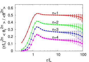
Figure 3: Moments of the coarse-grained scalar field $\langle\theta_{r}^{2n}\rangle$ compensated by the thermal equilibrium expectation $(r/L)^{2n}$. The errorbars are determined by dividing the sample in ten subsamples and computing the dispersion around the mean.

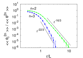
Figure 4: Cumulants of order 4 and 6 for the coarse-grained scalar field. The best fits for the slopes give exponents $5.32\pm 0.05$ for $n=2$ and $7.5\pm 0.5$ for $n=3$. The theoretical values $-16/3$ and $-22/3$ are shown for comparison.

Further insight on the deviations from statistical equilibrium at large scales can be gained by studying the statistics of the coarse-grained squared scalar field

$$\theta^{(2)}_{r}({\bm{x}},t)=\int G_{r}({\bm{x}}-{\bm{y}})\theta^{2}({\bm{y}},t)\,d{\bm{y}}\;.$$ (3)

The cumulants of $\theta^{(2)}_{r}$ give useful information about the presence of long-range correlations of the field $\theta^{2}$. The first-order cumulant $\langle\langle\theta^{(2)}_{r}\rangle\rangle\equiv\langle\theta^{(2)}_{r}\rangle$ is trivially equal to $\langle\theta^{2}\rangle$. The second-order cumulant $\langle\langle{\theta^{(2)}_{r}}^{2}\rangle\rangle=\langle{\theta^{(2)}_{r}}^{2}\rangle-\langle\theta^{(2)}_{r}\rangle^{2}$ for a scalar field in thermal equilibrium should decay rapidly to zero at large scales $r\gtrsim L$. On the contrary, as shown in Fig. 5, we observe a slow power-law decay with an exponent close to the theoretical expectation $\langle\langle{\theta^{(2)}_{r}}^{2}\rangle\rangle\simeq\langle\langle\theta^{4}\rangle\rangle(r/L)^{-4/3}$ FF04 .

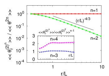
Figure 5: Cumulants of the coarse-grained, squared scalar field $\theta^{(2)}_{r}$. The definitions for the low-order cumulants of a generic random variable $z$ are: $\langle\langle z\rangle\rangle=\langle z\rangle$, $\langle\langle z^{2}\rangle\rangle=\langle z^{2}\rangle-\langle z\rangle^{2}$, $\langle\langle z^{3}\rangle\rangle=\langle z^{3}\rangle-3\langle z\rangle\langle z^{2}\rangle+2\langle z\rangle^{3}$, $\langle\langle z^{4}\rangle\rangle=\langle z^{4}\rangle-4\langle z\rangle\langle z^{3}\rangle-3\langle z^{2}\rangle^{2}+12\langle z^{2}\rangle\langle z\rangle^{2}-6\langle z\rangle^{4}$.

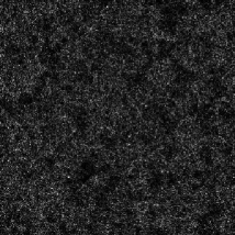
Figure 6: A snapshot of the squared scalar field $\theta^{2}$. Remark the inhomogeneous distribution of scalar intensity originating from long-range correlations $\langle\langle{\theta^{(2)}_{r}}^{2}\rangle\rangle\sim r^{-4/3}$.

Higher-order cumulants behave self-similarly as $\langle\langle{\theta^{(2)}_{r}}^{n}\rangle\rangle\sim\langle\langle{\theta^{(2)}_{r}}^{2}\rangle\rangle^{n-1}$. This result can be interpreted in terms of the geometrical properties of the positive measure defined by the squared scalar field: at scales $r\gtrsim L$ the field $\theta^{2}$ appears as a purely fractal object with dimension $D_{F}\approx 2/3$ (see Fig. 6). We end up by briefly discussing the physical origin of long-range scalar correlations. For a gaussian forcing we have $\theta^{2}({\bm{x}}_{1},t)\theta^{2}({\bm{x}}_{2},t)\stackrel{{\scriptstyle\Delta}}{{=}}F_{0}\phi_{1}^{2}\phi_{2}^{2}T_{1}T_{2}$. At distances $|{\bm{x}}_{1}-{\bm{x}}_{2}|=r\gg L$ the two gaussian variables $\phi_{1}$ and $\phi_{2}$ are independent. However, this is not the case for $T_{1}$ and $T_{2}$ because of the underlying velocity field. Therefore, the long power-law tail for $\langle\langle{\theta^{(2)}_{r}}^{2}\rangle\rangle$ arises from events where $\langle T_{1}T_{2}\rangle\gg\langle T\rangle^{2}$. This amounts to say that two blobs of initial size smaller than $L$, released at a distance $r\gg L$ in the same flow, do not spread considerably by turbulent diffusion (i.e. $T_{1,2}\gg\langle T\rangle$) with a probability $\sim(r/L)^{-4/3}$.

We acknowledge illuminating discussions with G. Falkovich and A. Fouxon. This work has been supported by the EU under the contract HPRN-CT-2002-00300. Numerical simulations have been performed at CINECA (INFM parallel computing initiative).

References

(1) U. Frisch, Turbulence, Cambridge Univ. Press,
Cambridge, (1995).
(2) G. Falkovich, K. Gawȩdzki, and M. Vergassola,
Rev. Mod. Phys. 73, 913 (2001).
(3) B. I. Shraiman and E. D. Siggia, Nature 405, 639 (2000).
(4) Z. Warhaft, Annu. Rev. Fluid Mech.32, 203 (2000).
(16) J. P. Gollub et al, Phys. Rev. Lett., 67, 3507, (1991).
(17) U. Frisch, A. Mazzino, A. Noullez, and M. Vergassola,
Phys. Fluids. 11, 2178 (1999).
(18) A. Celani and D. Vincenzi, Physica D 172, 103 (2002).
(19) B. I. Shraiman & E. Siggia, Phys. Rev. E, 49, 2912, (1994).
(20)
The statistics of the random variable
, where are independent and identically distributed random variables
with zero mean and finite variance ,
is completely characterized by the generating function . By virtue of statistical independency and identity in distribution
of the ’s, we have where is the generating function for .
For we have (a version of the central limit theorem) and therefore
.
The cumulants are defined
in terms of the Taylor series of around :
since we have .