Lattice Boltzmann method at finite-Knudsen numbers

Abstract

A modified lattice Boltzmann model with a stochastic relaxation mechanism mimicking “virtual” collisions between free-streaming particles and solid walls is introduced. This modified scheme permits to compute plane channel flows in satisfactory agreement with analytical results over a broad spectrum of Knudsen numbers, ranging from the hydrodynamic regime, all the way to quasi-free flow regimes up to $Kn\sim 30$.

The dynamic behaviour of flows far from hydrodynamic equilibrium is an important subject of non-equilibrium thermodynamics, with many applications in science and engineering. The non-hydrodynamic regime is characterized by strong departures from local equilibrium which are hardly handled on analytical means. Consequently, much work is being devoted to the development of computational techniques capable of dealing with the aforementioned non-perturbative and non-local effects. Recently, the lattice Boltzmann (LB) method has attracted considerable interest as an alternative to the discretization of the Navier-Stokes equations for the numerical simulation of a variety of complex flows LBE . Extending LB methods to non-hydrodynamic regimes is a conceptual challenge on its own, with a variety of microfluidic applications, such as flows in micro and nano electro-mechanical devices (NEMS, MEMS) CHI . Departures from local equilibrium are measured by the Knudsen number, namely the ratio of molecular mean free path, $l_{m}$, to the shortest hydrodynamic scale, $l_{h}$: $Kn=l_{m}/l_{h}$. Ordinary fluids feature $Kn<0.01$, while high Knudsen numbers are typically associated to rarefied gas dynamics, where $l_{m}$ is large because density is small, typical case being aero-astronautics applications. More recently, however, the finite-Kn regime is becoming more and more relevant for a variety of microfluidics applications in which the Knudsen number is large because of the increasingly smaller size of the devices. It is also worth emphasizing that the finite-Knudsen regime may also bear relevance to the problem of modeling fluid turbulence EU ; SCI . Recent work indicates that LB may offer quantitatively correct information also in the finite-Kn regime NIE . This hints at the possibility that LB may complement or even replace expensive microscopic simulation techniques such as kinetic Monte Carlo and/or molecular dynamics. On the other hand, this is also puzzling because finite-Knudsen flows are in principle expected to receive substantial contributions from high-order kinetic moments, whose dynamics is arguably not quantitatively correct because of lack of symmetry of the discrete lattice LL ; DELLAR . In this work we point out that, irrespectively of symmetry considerations, any LB extension aiming at describing non-hydrodynamic flows in the finite-Knudsen regime must first provide an adequate description of the dynamics of free-streamers, namely ballistic particles whose motion, in the limit of infinite Knudsen number, escapes any thermalization by either bulk or wall collisions.

This problem is connected to a pathology of the LB model, and in fact, of any discrete velocity model representing a whole set of molecular speeds within a finite solid angle, by a single discrete speed. The practical consequence of this drastic reduction of degrees of freedom in momentum space is a very efficient numerical scheme, but also the pathology connected to the fact that particles moving parallel to the wall (for example in a channel flow) never impact on the boundaries, so that under the effect of pressure gradients or body forces within the fluid flow, they may enter an unrealistic free-acceleration (runaway) regime. More generally, runaway must be expected whenever the particle mean free path exceeds the longest free-flight distance allowed by the geometrical set up.

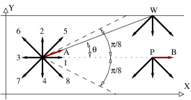
Figure 1: A simplified sketch showing the velocity structure for the D2Q9 model in a plane channel flow. In LBE models an hypothetic particle forming an angle $\theta$ with respect to the $\hat{x}$ axis (population “A”) is counted amongst the particles in population “1”. This particle would then, in the absence of collisions (i.e. for high-Knudsen numbers), be forced to stream parallel to the $\hat{x}$ axis without ever impacting on the walls. In real flows instead, its natural fate would be to move along a straight line until a collision with the wall would occurr at position “W”.

In this work we propose a mechanism to obviate this runaway pathology. Our method is demonstrated through the numerical simulations of a force-driven plane Poiseuille flow, as compared with existing analytical theories CERCI .

The lattice Boltzmann method has been described in detail in many publications, and here we shall only remind a few basic ideas behind this technique. The simplest lattice Boltzmann equation looks as follows LBGK :

$$f_{i}({\bm{x}}+\Delta t{\bm{c}}_{i},t+\Delta t)-f_{i}({\bm{x}},t)=$$ (1)

$$-\omega\Delta t[f_{i}({\bm{x}},t)-f_{i}^{e}({\bm{x}},t)]+F_{i}\Delta t$$

where $f_{i}({\bm{x}},t)\equiv f({\bm{x}},{\bm{v}}={\bm{c}}_{i},t)$, $i=1,\dots,n$, is the probability of finding a particle at lattice site ${\bm{x}}$ at time $t$, moving along the lattice direction defined by the discrete speed ${\bm{c}}_{i}$, and $\Delta t$ is the time step. The left-hand side of this equation represents free-streaming, while the right-hand side describes collisions via a simple relaxation towards local equilibrium $f_{i}^{e}$ (a local Maxwellian expanded to second order in the fluid speed) in a time lapse $\tau=\omega^{-1}$. This relaxation time fixes the fluid kinematic viscosity as $\nu=c_{s}^{2}(\tau-1/2)$, where $c_{s}$ is the sound-speed of the lattice fluid, ($c_{s}=1/\sqrt{3}$ in the present work). Finally, $F_{i}$ represents the effects of an external force. The set of discrete speeds must be chosen such that mass, momentum and energy conservation are fulfilled, together with rotational symmetry. Once these symmetries are secured, the fluid density $\rho=\sum_{i}f_{i}$, and speed ${\bm{u}}=\sum_{i}f_{i}{\bm{c}}_{i}/\rho$ can be shown to evolve according to the (quasi-incompressible) Navier-Stokes equations of fluid-dynamics. In this paper, we shall refer to the nine-speed D2Q9 model shown in Figure 1.

While at low Knudsen local equilibrium is established via bulk collisions, in the regime $Kn\geq 1$, the leading equilibration mechanism is provided by the interaction with the boundaries. Various types of boundary conditions have been used for LB simulations of finite-Knudsen flows BOON ; SLIP ; KWOK ; LIM . In this work, we confine our attention to bounce back (BB) BB and kinetic, as recently introduced by Ansumali and Karlin (AK) AK . The former implement no-slip flow speed at the wall via particle reflections, while the latter are based on the idea of reinjecting particles from the wall according to a local equilibrium distribution with wall speed and temperature. While AK were explicitly designed with finite-Knudsen effects in mind, this is clearly not the case for BB. At high-Knudsen, neither BB nor AK are expected to provide realistic results, since neither of them has been designed to do so.

It is therefore of interest to compare these two quite distinct types of boundary conditions throughout the full range of Knudsen numbers.

In a intermediate/high-Knudsen flow the main mechanism for thermalisation is provided by collisions with solid walls. This mechanism is non-local, meaning by this that, in order to be thermalized, a particle residing at a given lattice site (see population “A” in Fig. 1) needs to reach the wall (position “W” in Fig. 1), where it is scattered along some different direction, thereby transferring some momentum to the wall. From Figure 1 it is clear that in the LB representation, all molecules with momentum in the solid angle $[-\pi/8:\pi/8]$ around population “1”, are collapsed into population “1”. In the limit of infinite Knudsen numbers, population “1”, being parallel to the walls, behaves like a ballistic beam, whose motion escapes both bulk collisions and wall scattering. Due to the presence of an external drive, these beam particles enter a free-acceleration regime, which ultimately leads to runaway behaviour in time. Therefore, in the way to a finite-Knudsen LB scheme, no matter how accurate in terms of tensorial symmetry, a mechanism to thermalize these ballistic streamers needs to be introduced.

Here we propose a mechanism to mimick non-local wall collisions through virtual wall collisions (VWC for short). At every time step each free-streamer is assigned a virtual speed (called “A” in Fig. 1) $(v_{x},v_{y})=c\cdot(\cos\theta,\sin\theta)$, with $\theta$ uniformly distributed in $[-\pi/8,\pi/8]$. Assuming collisions are distributed according to a Poissonian, we define $p$ as the probability to “hit” (i.e. to collide at least once) the wall in a single time step, multiplied by the probability that no molecular collisions occurred during that time step. In practice, this means that a wall-collision event is performed at each time step and each lattice site with probability:

$$p(x,y;t)=e^{-1/Kn}\cdot\left(1-e^{-{{c\,dt\,\sin(\theta(x,y))}\over H}}\right)$$ (2)

where the first factor is the probability of undergoing no bulk collision during the flight of (average) length $H$ to the wall, when the average mean-free-path for bulk collisions is $\lambda$ (i.e. $-1/Kn=-\lambda/H$). The second term describes the fact that after a flight of length $L$ the particle hits the wall with probability one. This is modeled at each time step in the following way. In a time step $dt$ the particle moves a distance $dl=c\,dt$; since on average there is one collision every $L$ lattice spacings, the probability of a wall collision in a time step $dt$ is given by $\exp{(-dl/L)}=\exp{(-c\,dt\,\sin(\theta)/H)}$ (in our units $c\,dt=1$).

Note that $p$ goes to zero in the limit of $Kn\rightarrow 0$, so that virtual wall collisions fade away in the hydrodynamic regime, as they should. Due to the non-analytic dependence in $Kn$ the hydrodynamic limit is recovered faster than any power of $Kn$.

The probability $p$ goes to zero also in the limit $\theta\rightarrow 0$, corresponding to the case of the virtual speed falling back into a free-streamer (see Figure 1). However, by design, the occurrence of such a limit has now a vanishingly small probability, much like in a continuum flow.

Upon hitting the wall, the free-streamer feeds the span-wise moving populations according to the rules adopted for true wall-collisions (see Figure 1). For instance, for a virtual collision of a right-moving particle with the top wall, we have:

$$f^{\prime}_{1}=f_{1}(1-p),\;\;f^{\prime}_{7,8}=f_{7,8}+pf_{1}/6,\;\;f^{\prime}_{4}=f_{4}+2pf_{1}/3\;$$

where the coefficients $\{1/6,4/6,1/6\}$ correspond to the weights of the nine-speed local equilibrium.

Thanks to this mechanism, momentum is removed from populations aligned with the wall boundaries and re-distributed along the direction orthogonal to the boundaries. This allows the flow to relax towards a (non-local) equilibrium also in the limit of high $Kn$ numbers.

We simulate a two-dimensional flow in a rectangular duct of size $L$ along the streamwise direction ($x$) and width $H<L$ along $y$. The flow is driven by a volumetric force (force per unit volume) $F_{x}=\rho c\frac{8\nu U_{0}}{H^{2}}$ along the streamwise direction. In the hydrodynamic limit, such force leads to a parabolic velocity profile of amplitude $U_{0}$. Both BB and AK boundary conditions are applied on-site. The Knudsen number is tuned by changing the value of the viscosity, according to the expression:

$$Kn=l_{m}/H=\nu/(c_{s}H)$$

Knudsen numbers in the range $10^{-3}<Kn<30$ have been simulated, at a fixed Mach number $Ma=u/c_{s}=0.03$. The grid resolution used was $101\times 21$, although a few simulations at higher resolution of $101\times 41$ have also been performed to check the grid-independence of our results. After discarding the initial transient time, velocity profiles were averaged in time in order to minimize statistical fluctuations associated with the stochastic nature of the VWC mechanism.. The simulation was run until the relative change of the profiles fell below a given threshold (comparable with machine precision).

One of the major successes in the early days of kinetic theory was the prediction of a minimum of the mass flow rate as a function of the Knudsen number around $Kn\sim 1$. Interestingly, both BB and AK boundary conditions exhibit a minimum mass flow rate around $Kn\sim 1$ (see Figures 2 and 3). This indicates that, contrary to the common tenet, LB can capture the so-called “Knudsen paradox”. However, they both severely overestimate the mass flow in the high-Kn region, $Kn>1$. This is due to the presence of a finite fraction of ballistic streamers, as discussed earlier on. Figures 2 and 3 show the behaviour of the normalized mass flow rate $Q=\sum_{y}u_{x}(y)/(6\nu)$, for the case with and without virtual wall collisions.

The numerical results are compared with the analytical expression obtained by Cercignani in the zero and infinite Knudsen limits respectively (both fluxes are normalized in units of $6\rho\nu$):

$$Q_{0} = 1/(6Kn)+s+(2s^{2}-1)\;Kn$$ (3)

$$Q_{\infty} \sim \pi^{-1/2}\;\log{(Kn)}$$ (4)

where $s=1.015$ (see CERCI ).

Figure 2: AK boundary contions: normalized mass flux as a function of $Kn$ number, with ($\circ$) and without ($\blacktriangledown$) virtual wall collisions. The dashed line is Cercignani’s prediction (3) for low-$Kn$. Dotted lines are prediction (4) for high-$Kn$ multiplied by factors $1,2$ and $4$, from bottom to top. Following Cercignani, the mass flow is normalized with $6\rho\nu$.

Figure 3: BB boundary contions: normalized mass flux as a function of $Kn$ number, with ($\circ$) and without ($\blacktriangledown$) virtual wall collisions. Notations are the same as in the Figure 2.

.

By increasing the $Kn$ number the flow slips more and more, until the centerline speed becomes comparable with the sound speed, so that the LBE simulation breaks down.

As shown in Figure 2, by introducing virtual wall collisions, a nearly quantitative agreement with analytical results is observed. It is worth stressing that no free parameter has been used in the simulations. The highest achievable $Kn$ number may not be high enough to test the asymptotic prediction. Therefore, in order to appreciate the quality of our results, we have plotted Cercignani’s prediction, $Q_{\infty}$, in Figures 2 and 3, together with its magnifications by factors $2$ and $4$.

Back in 1867, Maxwell predicted that the slip length of a rarefied gas flowing on a semi-infinite slab should be proportional to the mean free path, $l_{s}=1.146Kn$, MAX . Nearly four decades ago, Cercignani computed the next order corrections in $Kn$, leading to the following quadratic expression for the slip speed:

$$V_{s}=aKn+bKn^{2}$$ (5)

where $a=1.146\cdot\left({{\partial u}\over{\partial y}}\right)_{y=-H/2}$ and $b=-0.9075\cdot\left({{\partial^{2}u}\over{\partial y}^{2}}\right)_{y=-H/2}$.

The dependence of the slip speed on the Knudsen number is presented in Figure 4. The slip velocity is defined as the value (at the wall position) of the parabolic fit of the averaged velocity profiles. Boundary data were excluded from the fit. The error bars on the slip velocity were estimated as the discrepancy between the results of the $21\times 101$ and $41\times 101$ simulations.

From Figure 4 it is clearly seen that BB boundary conditions fail to reproduce the slip velocity. Thus, our results support previous criticism on the use of BB boundary conditions at finite-Knudsen LUO ; AK . However, kinetic boundary conditions provide quantitative agreement with analytical results up to $Kn\sim 1$, even beyond the theoretical expectations. At intermediate and high Knudsen both BB and AK provide similarly inaccurate results. This is because the physics becomes more and more insensitive to the BB or AK boundary conditions and dependent on the VWC mechanism instead. Indeed, as virtual collisions are introduced, both BB and AK provide satisfactory agremeent with analytical data. The solid line in Figure 4 corresponds to the ratio $Q/(\rho H)$ and the fact that this quantity matches almost exactly the measured slip speed indicates that the flow profile is basically flat, as predicted by the asymptotic theory. Finally, our results do not extend below $Kn=0.01$ simply because an accurate evaluation of the very small values of $V_{s}$ in this regime requires a much higher transverse resolution than adopted here.

Figure 4: Wall slip velocity as a function of the Knudsen number for AK (plusses) and BB (triangles) boundary conditions. The solid line is the wall slip velocity extrapolated from the values of the flux computed assuming a flat velocity distribution across the channel. The dashed line is Cercignani’s low-Knudsen analytical prediction (5). Error bars as described in the text.

Our results indicate that a standard nine-speed LB scheme equipped with Ansumali-Karlin boundary conditions and a virtual wall collision mechanism, can capture salient features of channel flow in both hydrodynamic and strongly non-hydrodynamic regimes. Of course, this is only the first step towards a systematic inclusion of high-Knudsen effects in the lattice kinetic framework, and much further work is needed to address more general situations, such as non ideal geometries, high shear rates TRO and thermal effects GARCIA . Another interesting point to be explored for the future is the potential benefit of using multi-relaxation HSB ; MTR and entropic LB ELB schemes for a better description of fluid-wall interactions.

The authors thank S. Ansumali and I. Karlin for discussions and for making available their implementation of AK boundary conditions in a early stage of this project. SS acknowledge discussions with A. Garcia. Financial support from the NATO Collaborative Link Grant PST.CLG.976357 and CNR Grant (CNRC00BCBF-001) is acknowledged.

References

- (1) R. Benzi, S. Succi, M. Vergassola, Phys. Rep. 222, 145, 1992; D. Wolfe-Gladrow, “Lattice Gas Cellular Automata and Lattice Boltzmann Model”, Springer Verlag, 2000; S. Succi, “The Lattice Boltzmann equation”, Oxford Univ. Press, Oxford, (2001).
- (2) C.M. Ho, Y.C. Tai, Annu. Rev. Fluid Mech., 30, 579, 1998; G. Karniadakis, Microflows, Springer Verlag, 2001; P. Tabeling, Introduction a la microfluidique, Belin, 2003.
- (3) B.C. Eu, “Kinetic Theory and Irreversible Thermodynamics”, John Wiley and sons, New York, 1992.
- (4) H. Chen, S. Kandasamy, S. Orszag, R. Shock, S. Succi, V. Yakhot, Science, 301, 633, 2003.
- (5) X Nie, G. Doolen, S. Chen, J. Stat. Phys., 107, 29, 2002.
- (6) P. Lallemand, L.S. Luo, Phys. Rev. E, 61, 6546, 2001.
- (7) P. Dellar, Phys. Rev. E, 65, 036309, 2002.
- (8) C. Cercignani, “Theory and application of the Boltzmann equation”, Scottish Academic Press, 1975, chapter VI.
- (9) Y. Qian, D. d’Humières, P. Lallemand, Europhys. Lett. 17, 479, 1992.
- (10) P. Lavallée, J.P. Boon, Physica D, 47, 233, 1991.
- (11) S. Succi, Phys. Rev. Lett., 87, 96105, 2002.
- (12) B. Li and D. Kwok, Phys. Rev. Lett., 90, 124502, 2003.
- (13) C. Lim, C. Shu, X. Niu, Y. Chew, Phys. Fluids, 14, 2299, 2002.
- (14) S. Chen, D. Martinez, R. Mei, Phys. Fluids, 8, 2527, 1996.
- (15) S. Ansumali, I. Karlin, Phys. Rev. E, 66, 026311, 2002.
- (16) X. He, Q. Zou, L.S. Luo, M. Dembo, J. Stat. Phys., 87, 115, 1997.
- (17) J.C. Maxwell, Phil. Trans. Soc. London, 170, 231, 1867.
- (18) P.A. Thompson and S. Troian, Nature, (London) 389, 360, (1997).
- (19) Y. Zheng, A. Garcia, B. Alder, J. Stat. Phys., 109, 495, 2002.
- (20) F. Higuera, S. Succi, R. Benzi, Europhys. Lett., 9, 345, 1989.
- (21) D. d’Humieres, Progress in Astronautics and Aeronautics, 19, 450, 1992.
- (22) S. Ansumali, I.V. Karlin, J. Stat. Phys., 107, 291, 2002.