Excitability mediated by localized structures

Abstract

We find and characterize an excitability regime mediated by localized structures in a dissipative nonlinear optical cavity. The scenario is that stable localized structures exhibit a Hopf bifurcation to self-pulsating behavior, that is followed by the destruction of the oscillation in a saddle-loop bifurcation. Beyond this point there is a regime of excitable localized structures under the application of suitable perturbations. Excitability emerges from the spatial dependence since the system does not exhibit any excitable behavior locally. We show that the whole scenario is organized by a Takens-Bogdanov codimension-$2$ bifurcation point.

Localized structures (LS) in dissipative media have been found in a variety of systems, such as chemical reactions, gas discharges or fluids LS . They are also found in optical cavities, due to the interplay between diffraction, nonlinearity, driving, and dissipation LSoptical ; stephan . These structures, also known as cavity solitons have to be distinguished from conservative solitons found for example in propagation in fibers, for which there is a continuous family of solutions depending on their energy. Instead, dissipative LS are unique once the parameters of the system have been fixed. This fact makes this structures potentially useful in optical (i.e., fast and spatially dense) storage and processing of information stephan ; FirthScroggieOPN ; Coullet1 .

Localized structures may develop a number of instabilities like start moving, breathing or oscillating. In the latter case, they would oscillate in time while remaining stationary in space, like the oscillons found in a vibrated layer of sand oscillon . The occurrence of these oscillons in autonomous systems has been reported both in optical FirthPhSc ; josab ; longhi and chemical systems oscillonve .

In the present work we report on a route in which autonomous oscillating localized structures are destroyed, leading to a excitability regime. Excitability is a concept arising originally from biology (e.g. neuroscience), and it has been found in a variety of systems Excitreview , including optical systems opticalexcitab ; Plaza . Typically a system is said to be excitable if while it sits at an stable fixed point, perturbations beyond a certain threshold induce a large response before coming back to the rest state. In addition, excitability is also characterized by the existence of a refractory time during which no further excitation is possible. In phase space ErmenRinzel ; Izhikevich excitability occurs for parameter regimes where a stable fixed point is close to a bifurcation in which an oscillation is created. Possibly the best known example of an excitable system is FitzHugh-Nagumo model, close to the Hopf bifurcation, although one may also find excitable behavior mediated by a saddle point, namely either in the form of an Andronov (or saddle-node on the invariant circle) bifurcation or a saddle-loop (or homoclinic) bifurcation. These three possible scenarios are the simplest possible, occurring in systems that, minimally, can be characterized by two phase variables.

The concept of excitability has been extended to systems with spatial dependence by coupling several or many zero-dimensional excitable systems Excitreview . Here we consider a different situation: a system that without spatial dependence does not show excitable behavior while the localized structures that appear in the spatially dependent systems do.

A prototype model in nonlinear optics displaying the formation of LS is the one introduced by Lugiato and Lefever for an optical cavity filled with a Kerr medium Lugiato-Lefever . In the mean field approximation the dynamics of the scaled slowly varying amplitude of the complex field $E(\vec{x},t)$ is given by

$$\frac{\partial E}{\partial t}=-(1+i\theta)E+i\nabla^{2}E+E_{0}+i\left|E\right|^{2}E,$$ (1)

where $\nabla^{2}=\partial^{2}/\partial x^{2}+\partial^{2}/\partial y^{2}$. The first term describes cavity losses, $E_{0}$ is a homogeneous (plane wave) driving field, and $\theta$ the cavity detuning with respect to $E_{0}$. Eq. (1) has been normalized by the cavity decay rate, and it has a homogeneous steady state solution $E_{s}$ given implicitly by $E_{s}=E_{0}/(1+i(\theta-I_{s}))$, where $I_{s}=|E_{s}|^{2}$. We use the intra-cavity background intensity $I_{s}$ together with $\theta$ as convenient control parameters. The homogeneous solution has a instability leading to the formation of a hexagonal pattern at $I_{s}=1$. The bifurcation starts subcritically and the pattern coexists with the homogeneous solution Lugiato-Lefever ; Scroggie , so that a stable-unstable pair of LS is created in a saddle-node bifurcation Coullet1 . The unstable branch (the so-called lower or middle branch) has a single unstable direction. The region of existence of these LS, also known as Kerr cavity solitons, has been characterized in FirthPhSc ; josab , and is partially shown in Fig. 1. Increasing $\theta$, the LS undergoes a supercritical Hopf bifurcation and starts to oscillate autonomously FirthPhSc ; josab ; Skryabin . For one spatial dimension, Eq. (1) also exhibits LS in the appropriate parameter regime, but these structures do not undergo any Hopf bifurcation.

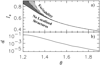
Figure 1: a) Phase diagram: $I_{s}$ vs. $\theta$. LS are stable in the shaded region and oscillate in the dashed one. Lines indicate bifurcations: saddle-node (solid), Hopf (dot-dashed), and sadle-loop (dashed). b) Distance between the saddle-node and Hopf lines.

As the control parameter $\theta$ is further increased part of the limit cycle moves closer and closer to the lower-branch LS, which is a saddle point in phase space, as illustrated in Fig. 2. On the left column we plot the time evolution of the LS maximum obtained from numerical integration of Eq. (1), the dashed line shows for comparison the maximum of the lower-branch LS. On the right column we sketch the evolution on phase space projected on two variables. At a certain critical value a global bifurcation takes place: the cycle touches the lower-branch LS and becomes a homoclinic orbit (Fig. 2c). This is an infinite-period bifurcation called saddle-loop or homoclinic bifurcation Gaspard . For $\theta>\theta_{c}$, the saddle connection breaks and the loop is destroyed (Fig. 2d). After following a trajectory in phase space close to the previous loop the LS approaches the saddle point (dashed line) where the evolution is dominated by its slow stable manifold (see the long plateau between $t=15$ and $t=60$ in Fig. 2d). Finally the LS decays to the homogeneous solution (dotted line). For larger values of $\theta$ the trajectory moves away from the saddle and, therefore, the decay to the homogeneous solutions takes place in shorter times.

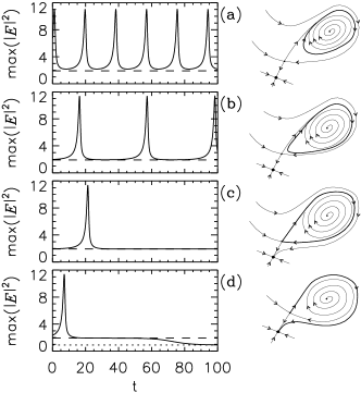
Figure 2: Left: LS maximum intensity as a function of time for increasing values of the detuning parameter $\theta$. From top to bottom $\theta=1.3,1.3047,1.30478592,1.304788$. $I_{s}=0.9$. Right: Sketch of the phase space for each parameter value. The thick line shows the trajectory of the LS in phase space.

The saddle-loop bifurcation has a characteristic scaling law that governs the period $T$ of the limit cycle as the bifurcation is approached. Close to the critical point the system spends most of the time close to the unstable LS (saddle). $T$ can be then estimated by the linearized dynamics around the saddle Gaspard

$$T\propto-{1\over\lambda_{1}}\ln(\theta_{c}-\theta),$$ (2)

where $\lambda_{1}$ is the unstable eigenvalue of the saddle point. We are now going to show that this scaling law is verified in our system. Fig. 3 shows the period of the LS limit cycle as a function of the control parameter $\theta$. As expected, the period of the limit cycle diverges logarithmically as the bifurcation is approached. We then evaluate $\lambda_{1}$ with arbitrary precision from a semi-analytical stability analysis of the unstable LS as in josab . The lower-branch LS has one single positive eigenvalue $\lambda_{1}=0.17713581$. In Fig. 3 (right) we plot using crosses the period of the oscillation LS as a function of $ln(\theta_{c}-\theta)$ obtained from numerical simulations of Eq. (1). Performing a linear fitting we obtain a slope $5.60$, in excellent agreement with the theoretical prediction $1/\lambda_{1}=5.65$, proving the existence of a saddle-loop bifurcation for the oscillating LS. We should note that the theory was developed for planar bifurcations, therefore, as the phase space is a plane, the saddle has one unstable direction and one attracting direction Gaspard . The stable manifold of the unstable LS is, however, infinite dimensional. The success of the planar theory to describe our infinite dimensional system can be attributed to the fact that, somehow, the dynamics of the LS is effectively two-dimensional with a single unstable manifold and an effective stable manifold.

Figure 3: a) Period of the limit cycle $T$ as a function of the detuning $\theta$ for $I_{s}=0.9$. The vertical dashed line indicate the threshold of the saddle-loop bifurcation $\theta_{c}=1.30478592$. b) Period $T$ as a function of $\ln(\theta_{c}-\theta)$. Crosses correspond to numerical simulations while the solid line has a slope $1/\lambda_{1}$ with $\lambda_{1}=0.177$ obtained from the linear stability analysis of the lower-branch LS.

In systems without spatial dependence it has been shown that an scenario composed by a saddle-loop bifurcation and a stable fixed point leads to a excitability regime ErmenRinzel ; Izhikevich ; Plaza . In our infinite-dimensional system LS does indeed show en excitable behavior: the homogeneous solution is a globally attracting fixed point but localized disturbances (above the lower-branch LS) can send the system on a long excursion through phase space before returning to the fixed point.

Fig. 4 shows the resulting trajectories of applying a perturbation in the direction of the unstable LS with three different intensities: one below the excitability threshold (dotted line), and two above: one very close to threshold (dashed line) and the other well above (solid line). In the first case the system relax exponentially to the homogeneous solution, while in the latter two cases it perform a long excursion before returning to the stable fixed point. In the case of a near threshold excitation the refractory period is appreciably longer due to the effect of the saddle. The spatial profile of the localized structure is shown in Fig. 4. The peak grows to a large value until the losses stop it. Then it decays exponentially until it disappears. A remnant wave is emitted out of the center dissipating the remaining energy.

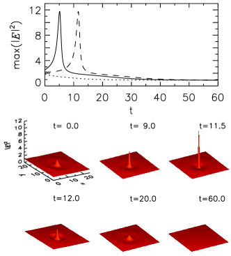
Figure 4: Evolution starting from the homogeneous solution ($I_{s}=0.9$) plus a localized perturbation of the form of the unstable LS multiplied by a factor $a$. Top panel shows the time evolution of the maximum intensity for $a=0.8$ (dotted line); $a=1.01$ (dashed line); $a=1.2$ (solid line). The $3D$ plots show the transverse profile at different times for $a=1.01$.

In absence of spatial degrees of freedom, Eq. (1) does not present any kind of excitability. This behavior is strictly related to the dynamics of the 2D LS. Eq. (1) is, in fact, a nonlinear Schrödinger equation (NLSE) with driving and damping. The phenomenon of self-focusing collapse NewellAkhmed of the 2D NLSE is behind the long excursion in phase space. When a localized perturbation concentrates enough power, the self-focusing nonlinear mechanism induces a concentration of energy at that place. In the absence of losses a collapse, i.e. a divergence of the energy concentration, would take place in a finite time collapse . However, the presence of losses prevents this collapse losses . The perturbation is finally dissipated and the system returns to the homogeneous solution. The same mechanism has also been used to explained the transport properties and dissipation rates in a wide class of turbulent flows Newell . The mechanism leading to excitability proposed in this letter is therefore not restricted to nonlinear optics. It may have implications in plasma physics and hydrodynamics, where coherent structures may have similar features as LS. Furthermore, LS appearing on different systems may undergo a Hopf bifurcation due to the nonlinear dynamics, even in the 1D case, as for example in parametrically amplified optical systems longhi .

In the limit of large detuning, the saddle-node, Hopf and saddle-loop bifurcation lines meet asymptotically, at $I_{s}=0$ as shown in Fig. 1. It is known that the intersection of a saddle-node line with a Hopf line is a Takens-Bogdanov (TB) codimension-2 bifurcation point Guckenheimer iff there is a double zero eigenvalue (the imaginary part of the Hopf vanishes as approaching the intersection with the saddle-node). The unfolding around a TB point leads to a saddle-loop bifurcation line Guckenheimer . So, this unfolding fully explains the observed scenario, where once again our formally infinite-dimensional system appears to be perfectly described by a dynamical system in the plane.

In Fig. 5 we plot the two eigenvalues with largest real part of the LS for parameter values corresponding to three vertical cuts of Fig. 1a). Open symbols indicate eigenvalues with a non-zero imaginary part while filled symbols correspond to real eigenvalues. Where open symbols cross zero in Fig. 5a) corresponds to the Hopf bifurcation while filled symbols crossing zero indicates the saddle-node bifurcation. For the three plots we have taken as origin the saddle-node bifurcation. The important point is that in the line of the two complex conjugate eigenvalues responsible of the Hopf bifurcation there is a place where the imaginary part vanishes leading to two real eigenvalues, the largest of which is precisely the responsible of the saddle-node bifurcation. As detuning increases the Hopf and saddle-node bifurcation points gets closer and closer but the structure of eigenvalues remains unchanged so that when the Hopf and saddle-node bifurcation will finally meet the Hopf bifurcation will have zero frequency, signaling a TB point.

The TB point occurs asymptotically in the limit of large detuning $\theta$ and small pump $E_{0}$. This limit corresponds to the case in which Eq. (1) becomes the conservative NLSE FirthLord . Details of the Hopf instability in this limit were studied in Skryabin , where there is evidence of the double-zero bifurcation point, but the unfolding leading to the scenario presented here is not analyzed.

Figure 5: Real (a) and imaginary (b) parts of the stable LS eigenvalues for three vertical cuts in Fig. 1 corresponding to detuning $\theta$: $1.7$ ($\Box$); $1.5$ ($\triangle$); $1.4$ ($\diamondsuit$) versus the difference between $I_{s}$ and its value at the saddle-node bifurcation $I_{s}^{s}(\theta)$.

In conclusion, we have analyzed an excitable regime associated to the existence of localized structures. We thus show that, in order to exhibit excitability, extended systems do not necessarily require to have local excitable behavior, instead such phenomenon can emerge due to the spatial dependence through the dynamics of a coherent (localized) structure. This open the possibility to observe excitable behavior in a whole new class of systems where excitability was not thought to be present. Coherent resonance Pikovsky-Kurths is also expected to be observed in theses systems upon application of localized disturbances of stochastic amplitude. Finally, localized structures have been shown to have a great potential as bits for optical memories stephan ; FirthScroggieOPN . This new excitable regimen opens also a new possibility for the use of localized structures as centers to process optical information in a similar way neurons do with electrical signals.

We thank G. Orriols for useful discussions. We acknowledge financial support from MEC (Spain) and FEDER: Grants BFM2001-0341-C02-02, FIS2004-00953, and FIS2004-05073-C04-03. DG acknowledges financial support from EPSRC (GR/S28600/01).

References

- (1) O. Thual and S. Fauve, J. Phys. (Paris) 49, 1829 (1988); J.E. Pearson, Science 261, 189 (1993); K.J. Lee et al., ibid. 261, 192 (1993); I. Müller, E. Ammelt, and H.G. Purwins, Phys. Rev. Lett. 82, 3428 (1999).
- (2) Feature section on cavity solitons, L.A. Lugiato ed., IEEE J. Quant. Elect. 39, #2 (2003); M. Tlidi, P. Mandel, and R. Lefever, Phys. Rev. Lett. 73, 640 (1994); B. Schäpers et al., ibid. 85, 748 (2000).
- (3) S. Barland et al., Nature 419, 699 (2002).
- (4) W.J. Firth and A.J. Scroggie, Phys. Rev. Lett. 76, 1623 (1996); W.J. Firth and C.O. Weiss, Opt. Photon. News 13, 55 (2002).
- (5) P. Coullet, C. Riera, and C. Tresser, Phys. Rev. Lett. 84, 3069 (2000); Chaos 14, 193 (2004).
- (6) P. Umbanhowar, F. Melo, and H.L. Swinney, Nature (London) 382, 793 (1996).
- (7) W.J. Firth, A. Lord, and A.J. Scroggie, Physica Scripta 67, 12 (1996).
- (8) W.J. Firth et al., J. Opt. Soc. Am. B 19, 747 (2002).
- (9) S. Longhi, G. Steinmayer, and W.S. Wong, J. Opt. Soc. Am. B 14, 2167 (1997).
- (10) V.K. Vanag and I.R. Epstein, Phys. Rev. Lett. 92, 128301 (2004).
- (11) E. Meron, Phys. Rep. 218, 1 (1992); J.D. Murray, Mathematical Biology, 3rd Ed. (Springer, 2002).
- (12) H.J. Wünsche et al., Phys. Rev. Lett. 88, 023901 (2002); A. Amengual et al. ibid. 76, 1956 (1996); S. Barland et al., Phys. Rev. E 68, 036209 (2003); J.L.A. Dubbeldam, B. Krauskopf, and D. Lenstra, ibid. 60, 6580 (1999).
- (13) F. Plaza et al., Europhys. Lett. 38, 85 (1997).
- (14) J. Rinzel and G.B. Ermentrout, in Methods in Neuronal Modeling, edited by C. Koch and I. Segev (MIT Press, Cambridge, MA, 1989).
- (15) E.M. Izhikevich, Int. J. Bif. Chaos 10, 1171 (2000).
- (16) L.A. Lugiato and R. Lefever, Phys. Rev. Lett. 58, 2209 (1987).
- (17) A.J. Scroggie et al., Chaos, Solitons, and Fractals 4, 1323 (1994).
- (18) D.V. Skryabin, J. Opt. Soc. Am. B 19, 529 (2002).
- (19) P. Gaspard, J. Phys. Chem. 94, 1 (1990); P. Glendinning, Stability, instability, and chaos (Cambridge U.P., Cambridge, UK, 1994); S. Strogatz, Nonlinear Dynamics and Chaos (Addison Wesley, Reading, MA, 1994).
- (20) A.C. Newell, Solitons in Mathematics & Physics (SIAM, Philadelphia, 1987); N.N. Akhmediev and A. Ankiewicz, Solitons: Nonlinear Pulses and Beams (Chapman and Hall, London, 1997).
- (21) J.J. Rasmussen and K. Rypdal, Phys. Scr. 33, 481 (1986).
- (22) M.V. Goldman, K. Rypdal, and B. Hafizi, Phys. Fluids 23, 945 (1980).
- (23) A.C. Newell, D.A. Rand, and D. Russell, Phys. Lett. A 132, 112 (1988).
- (24) J. Guckenheimer and P. Holmes, Nonlinear Oscillations, Dynamical Systems, and Bifurcations of Vector Fields (Springer, New York, 1983); Y. A. Kuznetsov, Elements of Applied Bifurcation Theory, 2nd ed. (Springer Verlag, New York, 1998).
- (25) W.J. Firth and A. Lord, J. Mod. Opt. 43, 1071 (1996).
- (26) A. Pikovsky and J. Kurths, Phys. Rev. Lett. 78, 775 (1997).